Operational cost and user performance analysis of on-demand bus and taxi systems

ABSTRACT

This paper presents the optimization problem of three different on-demand transit systems operated by vehicles of different sizes. This problem is aimed at minimizing the total cost of the system, which consists of the temporal cost experienced by users and the operating cost incurred by transit agencies. A compact set of estimations of the user performance and operating cost is provided, based on geometric probability. The optimization procedure allows the cost comparison of different semi-flexible services. Transit systems operated by cars (shared taxicabs) with flexible layouts are preferable for low demand densities (less than 92 pax/km²-h). For very high demand (higher than 200 pax/km²-h), bus systems with fixed layout and variable stop locations present the lowest total cost per passenger. In an intermediate domain, taxi and semi-flexible services compete among each other. The estimation of unit operating costs allows decision-makers to calculate the subsidies needed to make the system profitable.

KEYWORDS:

• On-demand transit services
• public transport
• flexible routes
• demand-responsive transport
• bus services
• taxis

Introduction

Mass transport (transit) is a key element for public administrations to alleviate the externalities associated with the increased use of private vehicles in terms of congestion, air pollution, noise, or accidents.

However, transit systems present high investment costs due to the deployment of infrastructure (e.g., dedicated lanes, terminals, stops). Their total operating costs are also significantly higher than those for individual modes (car, motorcycle, pedestrian, taxi). Nevertheless, the main strength of transit systems is their economies of scale: reducing infrastructure and operating costs per passenger as long as demand increases in the system. For this reason, the provision of mass public transport services (bus, tram, or rail) is only economically feasible for a potential demand beyond a minimum threshold. However, many factors influence the ridership of transit systems (Taylor and Fink 2013). The quality assessment provided in different studies (Dell’Olio, Ibeas, and Cecin 2011; Ojo 2019) is essential to understand how transit users perceive the importance of each service attribute. Based on that, transit operators may design user-oriented services to retain or even increase demand to establish funding schemes. In fact, optimal transit fares should be set equal to the marginal costs, which are low due to the economies of scale: usually, the fare paid by each user does not cover the unit cost per trip, justifying the existence of subsidies. In the current context of budgetary constraints of public authorities, decision-makers urge to reduce the operating costs of these collective transportation systems, especially when the expected demand flow is not significant (off-peak hours). This process has entailed a tailored allocation of resources to the expected users, providing some flexibility to the fixed layouts, stops pattern, and headways of public transport services, orienting to the demand needs.

Degrees of flexibility are very high and can trigger different services with different economic returns and acceptance by users. Daganzo (1978) was one of the first contributors providing analytical models for quantifying the performance and resources needed by different demand-responsive transportation services. From this time on, many studies have proposed specific designs of demand-responsive transport based on taxis (Salanova et al. 2011; Cuevas, Estrada, and Salanova 2016) or flexible buses (Kim, Schonfeld, and Kim 2018). Unfortunately, no works from the literature addressed how the service profitability would be guaranteed for transit agencies and the potential impact on subsidies, according to the demand density in each implementation. On-demand services may present different user performance metrics and operating costs for the same target transit demand density. They usually improve their performance and level of service to users at the expense of increasing the operating cost, and consequently, deploying more resources (Estrada and Robusté 2018). However, the travel time variability of these systems generates uncertainty in the service caused by detours of user’s pick-up. Bansal et al. (2019) analyze the impact of uncertain service time on demand. The economies of scale in these systems, when they exist, are not as noticeable as in transit services with fixed layout and headways. In recent years, several examples of on-demand collective transport have been observed in developed countries (Finland, New York, Barcelona, and others). However, some of these flexible bus initiatives have economically failed (Kutsuplus in Helsinki, reported in HSL-Helsinki Regional Transport Authority (2016); Chariot service in USA and London, reported in Hawkins 2019). Despite the fact that users welcomed and positively perceived these systems, the subsidies needed because of huge operating costs forced transit entities to cease the service. Transit agencies tended to underestimate the operating costs of the system for high demand rates, assuming similar economies of scale in collective transit systems with fixed services. Hence, the main motivation of this paper is to provide insights about the total cost of on-demand services concerning the expected demand and to set consistent fare and subsidies structures, ensuring the economic viability of the service. On-demand transit services are going to be launched in the Barcelona’s Metropolitan Area by AMTU (public entity that associates all the cities with urban transportation outside the metropolitan area of Barcelona) in the next 3 years (2022), extending to the whole Catalonia region. This entity and other transit agencies may need computational tools and models to estimate the unit fare and subsidies needed to run the service before its implementation.

Therefore, this paper analyzes the optimal service design of three on-demand transit systems operated by vehicles of different capacities with different levels of flexibility, regarding the spatial configuration of the route and the temporal coverage. The optimization problem is aimed at minimizing the total cost of the on-demand transportation system, which includes user and transit agency cost, with regard to stop distances, headways, or maximal user waiting time decision variables. The vehicle size considered ranges from medium-capacity buses available on the market (70 pax) to passenger cars (5 pax). An analytic model is presented where user performance metrics and operating costs are estimated using continuous approximation methods. Continuous approximation methods require less computational time and accurate data sets to obtain a solution, compared to combinatorial optimization techniques. Moreover, they are able to highlight cause–effect relationships and managerial insights for large problems (Ansari et al. 2018; Askari et al. 2020). Nevertheless, due to the discrete nature of transportation problems in real life, some variables of the problem (for example, the fleet size) should be rounded up or down to the next feasible integer number. The objective function is convex and presents a flat and smooth domain around the optimal solution. The agreement between the solution obtained in the continuous and integer problems is good when the optimal values of these variables are big enough. However, when optimal values are close to 0, the goodness of the solution in real implementations is not justified and it should be checked. In Estrada and Roca-Riu (2017), the corresponding mixed-integer version for the Vehicle Routing Problem is formulated using a continuous approximation approach. Despite the fact that we lose the clarity of the managerial insights, the optimal solutions in the continuous and mixed problem do not differ significantly, even for small values of variables.

The modeling approach in this paper is based on the metrics developed for individual modes such as taxi systems (Salanova and Estrada 2018) and semi-flexible bus routes (Nourbakhsh and Ouyang 2012; Papanikolaou and Basbas 2020). These models have been partially modified to consider the same input parameters, decision variables, and area of implementation. These models have been developed for three on-demand services. In the service called STOP, the transit agency is able to modify the number of stops depending on the target demand. Although the layout of the route is given, transit vehicles may skip those stops where there are no boarding or alighting passengers. The second service, known as LAYOUT, presents a flexible route layout to visit every origin and destination of users, to be served by the same vehicle. Therefore, each vehicle carries multiple customers in the same roundtrip but they only stop at user pick-up and dropping points. Finally, DIRECT service is an individual means of transport from many origins to many destinations. Every user trip is allocated to a single exclusive vehicle, providing a service without any intermediate stop. STOP and LAYOUT services may require vehicles of different capacities, depending on the expected occupancy. In this study, the fleet typology considered encompasses passenger cars, minibuses and medium-capacity buses of diesel, hybrid and electric powertrains. On the contrary, as DIRECT service is exclusively provided to a single customer, we only consider passenger cars (manned or unmanned).

Therefore, the analytical models developed for STOP, LAYOUT, and DIRECT services are able to identify the most efficient flexible design among three on-demand service typologies to minimize the total system cost and compare their cost and performance to other tailored services for the same target demand. In this paper, we identify the demand domain in which each kind of on-demand service provides a minimal solution in terms of the total cost. These models also allow determining the farebox recovery ratio and the necessary subsidies from the administration to guarantee the profitability of the operation (when fares are defined) or the minimal fare to make the system profitable. Nevertheless, other performance aspects affecting the perceived quality of on-demand users (driver behavior, vehicle condition) should be assessed by principal component analysis and structural equation models (Askari et al. 2020). An application to an urban area under different demand densities is also presented, considering the input cost parameters of Barcelona’s Metropolitan Area.

Modeling framework

In this paper, we assume that all on-demand transportation services will be deployed in a rectangular-shaped corridor of length L and width w. It may represent the vast majority of real bus corridor implementations. Although the DIRECT service may be deployed in urban areas of alternative shapes, we restrict the analysis in rectangular service areas, to compare the performance of the aforementioned services under the same conditions. The three on-demand services are depicted in Figure 1. The design models presented in this paper are aimed at identifying the optimal equilibrium in the service design using continuous approximations, balancing a competitive door-to-door travel time and an affordable operating cost of transit systems (Estrada et al. 2011).

Figure 1. Route schemes of flexible services. STOP Service-Route with a fixed layout and variable location of stops, LAYOUT Service-Route with variable layout, DIRECT Service- Taxi managed by a dispatching center

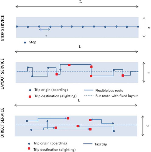
The performance and cost formulations are estimated considering the following assumptions:

1. All services are provided over the same area of the city R (km²), which is assumed to be equivalent to R = L·w. In the case that transit agencies are willing to deploy DIRECT service in a region of different shapes, the variable R can be replaced by the corresponding real area of this service region. The demand density ${\lambda }_d$(pax/h-km²) of passengers’ trip origins is constant and uniformly distributed in the area $R$.

2. In-vehicle and walking distances $d_{\gamma }$are calculated by grid distance metric in Cartesian coordinates between origin (1) and destination (2) points, $d_{\gamma }=\left|\left(x_2-x_1\right)+\left(y_2-y_1\right)\right|$.

3. The calculation of passenger trip destinations considers the length of each trip performed by a single user is l < L along the longitudinal direction of the bus route and w/3 in the transversal direction.

4. The street network presents a perfect grid configuration. The spacing between streets in two orthogonal directions is $\mathrm{\Delta }b$ (km).

5. The decision variable in collective services (STOP and LAYOUT) is the time headway (H, in hours). In service STOP, there is also a second decision variable: the spacing between consecutive stops (s, in km). In DIRECT service, the decision variable is the maximal user’s waiting time T₀ (in hours), which also represents the temporary coverage of the service.

6. The amount of stops in STOP service along the roundtrip is variable and depends on the hourly demand density. The number of effective stops S_e in the roundtrip performed by a vehicle is calculated by Equation (1)(1) $\begin{array}{c}\begin{array}{c}{S}_e={\left[2{\lambda }_{d}RH\right]}^{+}if2{\lambda }_{d}RH<\frac{2L}{s}\\ S_e={\left[\frac{2L}{s}\right]}^{+}if2{\lambda }_{d}RH\ge \frac{2L}{s}\end{array}\\ \end{array}$(1) . If the number of boarding and alighting operations (i.e., two times the total number of passengers served) is lower than the number of predefined stops spaced at s spacing (first case of Equation 1(1) $\begin{array}{c}\begin{array}{c}{S}_e={\left[2{\lambda }_{d}RH\right]}^{+}if2{\lambda }_{d}RH<\frac{2L}{s}\\ S_e={\left[\frac{2L}{s}\right]}^{+}if2{\lambda }_{d}RH\ge \frac{2L}{s}\end{array}\\ \end{array}$(1) ), we assume that vehicles are not going to stop over every predefined boarding/alighting point. The second condition represents the opposite case, where more than one user will get on/get off the vehicle at each predefined stop.

(1) $\begin{array}{c}\begin{array}{c}{S}_e={\left[2{\lambda }_{d}RH\right]}^{+}if2{\lambda }_{d}RH<\frac{2L}{s}\\ S_e={\left[\frac{2L}{s}\right]}^{+}if2{\lambda }_{d}RH\ge \frac{2L}{s}\end{array}\\ \end{array}$(1)

1. The maximal cruising speed of vehicles in the area is v for all services. The walking speed of users to access and egress stops is constant and equal to $v_w$. The vehicles that operate STOP and LAYOUT services have a constant deceleration -a in the braking phase before arriving at a stop. The same acceleration rate, a (with opposite sign), is achieved when leaving the stop until reaching the cruising speed v again. Therefore, the performance of a stop penalizes the travel time of transit vehicle with $\tau =\frac{v\left(k\right)}{a}$. The boarding and alighting time per passenger is constant and equivalent to $\tau { }^{\mathrm{\prime }}$. The door’s opening and closing time at stops are considered to be instantaneous. Appendix 1 presents the glossary of all terms and variables.

Operating cost metrics

The operating costs of the flexible transport system in 1 hour of service ($Z_A$, in EUR/h) can be estimated according to Equation (2)(2) $Z_A=c_{d}Q+c_{t}M$(2) , where M (veh-h/h) is the number of required vehicles and Q (veh-km/h) the distance traveled by the fleet in 1 hour of service. The input parameters $c_d$(EUR/veh-km) and $c_t$ (EUR/veh-h) should be defined for each implementation. The former parameter embraces all operating cost components that vary according to the distance run by each vehicle. On the contrary, the latter considers all fixed cost components of each vehicle, such as vehicle depreciation, salaries, insurances, etc. Finally, the terms Q and M depend on the decision variables of the problem and present specific formulations for each on-demand service. Then, we can calculate the farebox recovery ratio, η, that relates the average fare income of an average trip and the mean operating cost of this trip $z_P$. The mean cost of a trip can be quantified by $z_P=Z_A/\left({\lambda }_{d}R\right)$. The analytical estimation is given by $\eta =\theta /z_P$ in the flexible STOP and LAYOUT services, where $\theta$ is the average fare per trip. In the DIRECT service, the ratio is given by $\eta =\left(l\cdot {\theta }_{km}+\mathrm{\Phi }\right)/z_P$, where ${\theta }_{km}$ and $\mathrm{\Phi }$ are, respectively, the fare per kilometer and the flag-drop fee at which each trip of length $l$ is charged.

(2) $Z_A=c_{d}Q+c_{t}M$(2)

User costs metrics

The costs that users experience while using the collective transport system ($Z_U$ in Equation 3)(3) $Z_U=\left(A+W+IVTT\right){\beta }_T{\lambda }_{d}R$(3) are quantified as the product of total door-to-door time, the perceived value of travel time ${\beta }_T$, demand density of users λ_d and the area of service R. The door-to-door travel time is assumed to be the linear sum of the expected access (A), stop waiting (W), and the in-vehicle travel time (IVTT) of a single user.

(3) $Z_U=\left(A+W+IVTT\right){\beta }_T{\lambda }_{d}R$(3)

The components of the door-to-door travel time present different formulations depending on the typology of on-demand service considered. For example, the access time A is only different from 0 for the on-demand STOP service. In other services, each vehicle picks passengers up at his/her trip origin, and passengers do not have to walk. For the sake of simplicity, we assume that the cruising speed of transit vehicles in all services is constant and given by $v$and, therefore, it is not affected by how many vehicles are in operation. In El Esawey and Sayed (2011), some insights about the estimation of bus cruising speeds are provided.

Estimation of user and agency cost components in STOP service

Assuming the band of Figure 1, the total hourly passenger flow will be evenly distributed in λ_dLw/2 trips per hour through the East and λ_dLw/2 trips to the West direction. Passengers are assumed to board and alight from buses at given stops, whose spacing is s (km). Users indicate the stop where they want to get on or get off the bus before the bus arrival at this stop. Therefore, a single bus can skip those stops if there is no request of passengers.

Access time, A. The maximal access distance from any point in the service area to the transit stop is s/2 in the longitudinal direction and w/2 in the transversal direction, respectively. The expected value of the access distance is calculated by $E\left(d\right)=\underset{l{x}_{min}}{\overset{l{x}_{max}}{\int }}xf\left(x\right)dx+\underset{l{y}_{min}}{\overset{l{y}_{max}}{\int }}yf\left(y\right)dy,$where (x, y) is the location of the origin of the trip in the domain $l{x}_{min}\le x\le l{x}_{max}$, $l{y}_{min}\le y\le l{y}_{max}$ and f (x), f (y) are the distribution density functions of the variables x and y. For a uniform distribution where $f\left(x\right)=\frac{1}{l{x}_{max}-l{x}_{min}}$, $f\left(y\right)=\frac{1}{l{y}_{max}-l{y}_{min}}$, and the maximal and minimal domain values $l{x}_{max}=s/2$, $l{y}_{max}=w/2$, $l{x}_{min}=l{y}_{min}=0$; therefore, the expected value of the access distance between a stop and a trip origin location is E(d) = s/4 + w/4. Finally, assuming the walking speed of users is equal to v_w, the estimation of access and egress time (from the last stop to the final destination) is through by Equation (4)(4) $A=2E\left(d\right)/v_w=\left(s+w\right)/\left(2v_w\right)$(4) .

(4) $A=2E\left(d\right)/v_w=\left(s+w\right)/\left(2v_w\right)$(4)

Waiting time, W. We assume that, with the current technology, users know the arrival time of vehicles at each stop or location. We also assume that vehicles are dispatched at regular time headways from the first stop. Nevertheless, arrivals of vehicles at intermediate stops may be slightly irregular, depending on the boarding demand on the previous stops. We assume that each arrival i of transit vehicles at a given stop presents a temporal gap (headway) with the predecessor vehicle defined by H_i, where the subscript defines the reference of the arrival sequence. In a first approximation, we will consider a constant passenger arrival rate λ_p (pax/h) at stop p. Assuming that the vehicles have sufficient vehicular capacity to enable all waiting passengers to board, and, the boarding operation is instantaneous, the total number of passengers boarded in the first K headways can be expressed by $N\left(T_w\right)=\sum _{i=1}^K{\lambda }_p{H}_i^{\hspace{0.17em}}$, where $T_w$denotes the period length $T_w=\sum _{i=1}^K{H}_i^{\hspace{0.17em}}$. Similarly, the total waiting time in the $T_w$ period, measured in passenger hour, is determined by $\mathrm{\Omega }\left(T_w\right)=\sum _{i=1}^K\frac{{\lambda }_p{H}_i^2}{2}$. Hence, the average waiting time per passenger is defined by $W=\frac{\mathrm{\Omega }\left(T_w\right)}{N\left(T_w\right)}=\frac{1}{2}\frac{{\sum }_{i=1}^K{H}_i^2}{{\sum }_{i=1}^K{H}_i^{\hspace{0.17em}}}$, which is independent of λ_p. The previous quotient can be conceived as the expectation of variable $H_{\hspace{0.17em}}^2$divided by the expectation of variable$H$. The numerator can be replaced by the expression that relates the variance of a random variable x to the expectations of the variable itself x and x², $E^2\left(x\right)=E\left(x\right)+Var\left(x\right)$. Finally, the waiting time can be rewritten by Equation (5)(5) $W=\frac{1}{2}\left(\bar{H}+\frac{s_H^2}{\bar{H}}\right)$(5) . In this expression, $\bar{H}$ denotes the average time headway and $s_H^2$the variance of headways H_i, i = 1, K.

(5) $W=\frac{1}{2}\left(\bar{H}+\frac{s_H^2}{\bar{H}}\right)$(5)

In-Vehicle travel time, IVTT. The commercial speed of vehicles is computed as the total trip length l divided by the time Tr needed to overcome this distance. This time is divided into three components, similarly to Daganzo (2010):

1. the time needed to travel the distance l assuming that the vehicle does not stop over intermediate stations. Therefore, it keeps the constant cruising speed along the service. This component is easily estimated as l/v.

2. the time spent at all stops along l to slowdown, stop the vehicle, and then accelerate until it reaches the cruising speed v again. This component is quantified as the product of the number of stops that a vehicle will perform along l, and, the additional time τ consumed in the braking and acceleration operation at each stop, with regard to a vehicle that moves at a constant cruising speed. From Daganzo (2010), we know that this time is equivalent to $=\frac{v}{a}$.

3. the time needed by users to get on and off the vehicle along l. If the unit boarding and alighting time per user is τ’ (hours/pax), the total time spent at stops due to passenger boarding and alighting operations along l is $\frac{{\lambda }_d}{2L}{\tau }^{\prime }$.

The commercial speed of vehicles is $v_c=\frac{l}{T_r}={\left(\frac{1}{v}+\frac{S_e}{2L}\frac{v}{a}+\frac{1}{L}\frac{{\lambda }_d}{2}{\tau }^{\prime }\right)}^{-1}$. In this way, the in-vehicle travel time IVTT to perform a trip of length l can finally be estimated by Equation (6)(6) $IVTT=E\left(\frac{l}{v_c}\right)=\frac{l}{v}+\frac{l}{2L}{S}_e\frac{v}{a}+\frac{l}{L}\frac{{\lambda }_{d}RH}{2}\tau \prime$(6) .

(6) $IVTT=E\left(\frac{l}{v_c}\right)=\frac{l}{v}+\frac{l}{2L}{S}_e\frac{v}{a}+\frac{l}{L}\frac{{\lambda }_{d}RH}{2}\tau \prime$(6)

Total distance traveled by the fleet in 1 hour, Q. Recalling that the length of the roundtrip is 2 L, there will be a vehicle that has completed an entire roundtrip, i.e. has traveled a distance 2 L, at each time headway H. Therefore, the distance traveled by the fleet per unit time is given by Equation (7)(7) $Q=\frac{2L}{H}$(7) .

(7) $Q=\frac{2L}{H}$(7)

Fleet size, M. The number of vehicles needed to maintain the target headway H can be estimated as the quotient between the roundtrip travel time and the headway H. Assuming that the roundtrip travel time is equivalent to the route length divided by the commercial speed; the fleet size is calculated by Equation (8)(8) $M=\frac{2L}{H{v}_c}=\frac{2L}{H}{\left(\frac{1}{v}+\frac{S_e}{2L}\frac{v}{a}+\frac{1}{L}\frac{{\lambda }_{d}RH}{2}{\tau }^{\prime }\right)}^{\hspace{0.17em}}$(8) .

(8) $M=\frac{2L}{H{v}_c}=\frac{2L}{H}{\left(\frac{1}{v}+\frac{S_e}{2L}\frac{v}{a}+\frac{1}{L}\frac{{\lambda }_{d}RH}{2}{\tau }^{\prime }\right)}^{\hspace{0.17em}}$(8)

Vehicle occupancy, O. The demand density in a corridor direction is ${\delta }_l=\frac{{\lambda }_{d}R}{2L}$. Thus, the passenger flow in a given section will be equivalent to all travelers who have got on the bus in the segment of length l prior the section (upstream). Therefore, the passenger flow of in any section will be $q\left(\frac{pax}{hour}\right)=\frac{l{\lambda }_{d}R}{2L}$and, if multiplied by the headway H, the occupation of the vehicle (in pax/veh) is finally obtained by Equation (9)(9) $O=\frac{l{\lambda }_{d}R}{2L}H$(9) .

(9) $O=\frac{l{\lambda }_{d}R}{2L}H$(9)

Estimation of user and agency cost components in LAYOUT service

In this case, we consider a route with a flexible layout along a corridor of length L and a transverse width of service w, as in STOP service, with a passenger demand density λ_d. We assume that origins and destinations are uniformly distributed over the corridor area R = L ·w. The route layout in each roundtrip visits all origins and destinations of the users requiring service. The developed formulas have been adapted from the work of Nourbakhsh and Ouyang (2012).

Total distance traveled in 1 hour, Q. This metric is evaluated as a sum of three components: the longitudinal distance, a transversal distance within the band, and an additional detour distance according to the available streets. The longitudinal distance run by one vehicle along the corridor will be equivalent to the STOP service and equal to 2 L. The transversal distance between two consecutive points can be computed as the expected distance between two points uniformly distributed along a segment of length w, i.e. w/3 (Daganzo 1984). This metric should be multiplied by the total number of boarding and alighting operations in the roundtrip, i.e. $2{\lambda }_{d}RH$ . The estimation of the extra detour distance assumes an orthogonal street network, where the mesh space between streets is ∆b > 0. If there are two or more trip origins or destinations in the same street block, the bus travels an extra longitudinal distance. The expected additional distance to visit a new demand point in the same street block is ∆b/2. We consider that the number of trip origins and destinations within the same street block in a forward route direction follows a uniform distribution. The probability of performing one stop in the street block of area ∆bw (i.e., one origin or destination point) is 2∆bw/(Lw). Therefore, the probability P{i} of having a total number of i origin and destination points within the same block is defined by $P\left\{i\right\}={\left(\frac{2\mathrm{\Delta }bw}{wL}\right)}^i$. Therefore, in case there are i> 2 trip origins or destinations in the same block, the bus will have to cover an extra distance of $\left(i-1\right)\frac{\mathrm{\Delta }b}{2}$ per vehicle and street block. Taking into account this extra distance for all blocks along the corridor, the total extra distance is $D_e=L\sum _{i=2}^{\mathrm{\infty }}\left(i-1\right)P\left\{i\right\}$. It should be noted that the length of each block ∆b has been replaced by the total length of the corridor 2 L. Finally, the distance traveled by the fleet per hour is given by the ratio between the summation of the former distance components and the time headway (Equation 10(10) $Q=\frac{1}{H}\left(2L+\frac{2{\lambda }_{d}LH{w}^2}{3}+L\sum _{i=2}^{\mathrm{\infty }}\left(i-1\right)P\left\{i\right\}\right)$(10) ).

(10) $Q=\frac{1}{H}\left(2L+\frac{2{\lambda }_{d}LH{w}^2}{3}+L\sum _{i=2}^{\mathrm{\infty }}\left(i-1\right)P\left\{i\right\}\right)$(10)

Fleet size, M. The number of vehicles required to operate the route at a given headway H can be estimated as the quotient between the total distance traveled in 1 hour and the average commercial speed of vehicles $M=\frac{Q}{v_c}$. The commercial speed is then evaluated by Equation (11)(11) $\frac{1}{v_c}=\frac{1}{v}+\frac{2{\lambda }_{d}RH}{QH}\frac{v}{a}+\frac{{\lambda }_{d}RH\tau { }^{\mathrm{\prime }}}{QH}$(11) .

(11) $\frac{1}{v_c}=\frac{1}{v}+\frac{2{\lambda }_{d}RH}{QH}\frac{v}{a}+\frac{{\lambda }_{d}RH\tau { }^{\mathrm{\prime }}}{QH}$(11)

The first component of Equation (11)(11) $\frac{1}{v_c}=\frac{1}{v}+\frac{2{\lambda }_{d}RH}{QH}\frac{v}{a}+\frac{{\lambda }_{d}RH\tau { }^{\mathrm{\prime }}}{QH}$(11) represents the time needed to travel one kilometer at maximum speed. The second term represents the time lost per kilometer in the braking and acceleration operation before/after stops, in comparison to a vehicle traveling at a constant speed. The term $\frac{2{\lambda }_d}{QH}$ is the number of stops visited per each vehicle and kilometer. The term QH is indeed the total roundtrip distance of a single vehicle, also considering the transversal and detour component of the route. Finally, the third term in Equation (11)(11) $\frac{1}{v_c}=\frac{1}{v}+\frac{2{\lambda }_{d}RH}{QH}\frac{v}{a}+\frac{{\lambda }_{d}RH\tau { }^{\mathrm{\prime }}}{QH}$(11) addresses the time spent in boarding/alighting operations per kilometer.

Access time, A. The service definition involves vehicles visit the origins and destinations of user trips. Therefore, access time will be negligible, A = 0.

Waiting time, W. As in the previous STOP service, a single user is supposed to wait W units of time given by Equation (5)(5) $W=\frac{1}{2}\left(\bar{H}+\frac{s_H^2}{\bar{H}}\right)$(5) .

In-vehicle travel time, IVTT. In this case, the IVTT variable will be calculated by considering the transversal distance and additional detour distance of the bus motion. We assume that the length of a single trip in the longitudinal distance of the route is l. Therefore, from the total roundtrip distance QH/2 of a single bus, we will only consider the l/L ratio that a single user is going to perform. In this sense, the expected distance between a trip origin and destination (sum of longitudinal, lateral, and extra distances) can be approximated by $E\left(l\right)=\frac{QHl}{2L}$. Finally, the in-vehicle travel time is defined by Equation (12)(12) $IVTT=E\left(\frac{l}{v_c}\right)=\frac{QHl}{2L}\left(\frac{1}{v}+\frac{2{\lambda }_{d}RH}{QH}\frac{v}{a}+\frac{{\lambda }_{d}RH\tau { }^{\mathrm{\prime }}}{QH}\right)$(12) .

(12) $IVTT=E\left(\frac{l}{v_c}\right)=\frac{QHl}{2L}\left(\frac{1}{v}+\frac{2{\lambda }_{d}RH}{QH}\frac{v}{a}+\frac{{\lambda }_{d}RH\tau { }^{\mathrm{\prime }}}{QH}\right)$(12)

Vehicle occupancy, O. Following the same approach as in the STOP service, the occupancy in the critical section of the route is given by Equation (9)(9) $O=\frac{l{\lambda }_{d}R}{2L}H$(9) .

Estimation of user and agency cost components in DIRECT Service

We assume that a taxi service is provided in a region of area R, where λ_d passengers are uniformly distributed per unit of area and time. Users call a dispatching center that assigns the vacant taxi nearest to the current location of a customer. Then, the taxi goes to this location (assigned phase) to pick up the customer and carry him/her to the final destination, overcoming a trip length l_t in any direction in R. In order to be consistent to STOP and LAYOUT service, this trip length should be l_t = l + w/3, where l as the trip length in the longitudinal direction of the route layout. In STOP service, the in-vehicle trip length was l, although the user has to overcome an additional w distance by foot in the access and egress leg of the trip. In Direct service, this distance is travelled onboard the taxi.

Fleet size, M. In this flexible mode of transport (unlike the STOP and LAYOUT services discussed above), vehicles are not dispatched at a regular frequency (there is no headway to be met). Taxi vehicles will be dispatched when users call to order a service. As it is discussed in Daganzo (2010), the size of the taxi fleet can be divided into three types of states: number of free/vacant taxis, number of assigned taxis (they are moving to the customer location), and the number of taxis in service. The taxi fleet will be sized to meet the target user’s wait time, i.e. the period between the time the taxi is requested and the moment when it picks the user up. This target parameter is denoted by T₀. Imposing the equilibrium condition in the vehicle transitions among all potential states (vacant, assigned, and in service) and queue theory, Daganzo (2010) defines the expected number of vehicles in each state. Hence, the number of vacant, assigned, and in-service vehicles are respectively evaluated by $n_i=\frac{R}{{\left[2v\left(T_0-t_a\right)\right]}^2}$, $n_a=\lambda R{T}_0$ and $n_s=\lambda R\left(\frac{\mathrm{\ell }}{v}+\frac{w}{3v}+t_{\theta }\right)$, where v is the cruising speed, $t_a$ is the time needed by the dispatching center to assign each call to one vacant taxi, and $t_{\theta }$ is the time needed by the user to pay for the service and get off the taxi. Finally, the total fleet size, as a sum of $n_a$, $n_s$and $n_i$, is given by Equation (13)(13) $M=\frac{R}{{\left[2v\left(T_0-t_a\right)\right]}^2}+{\lambda }_{d}R\left(T_0+\frac{\mathrm{\ell }}{v}+\frac{w}{3v}+t_{\theta }\right)$(13) .

(13) $M=\frac{R}{{\left[2v\left(T_0-t_a\right)\right]}^2}+{\lambda }_{d}R\left(T_0+\frac{\mathrm{\ell }}{v}+\frac{w}{3v}+t_{\theta }\right)$(13)

Distance traveled in 1 hour, Q. It can be verified that for each trip served by the taxi system, the vehicle will have to travel a distance l + w/3 in service (with the client onboard) and an access distance $d_n=\frac{1}{2v}\sqrt{\frac{R}{n_i}}$ from the former vehicle position to the customer’s location. This statement is valid only if the vehicle, after a customer’s service, is not mobilized. Indeed, the distance $d_n$ should be run within the target waiting time defined by the taxi manager. Therefore, in order to minimize the number of resources needed, we impose $d_n=T_{0}v$. Under this situation, the distance traveled for each trip is $\left(l+\frac{w}{3}+v{T}_0\right)$. Since we have a total of R·λ_d trips per hour of service in the study area, the total distance traveled by the taxi fleet will be defined by Equation (14)(14) $Q={\lambda }_{d}R\left(l+\frac{w}{3}+v{T}_0\right)$(14) .

(14) $Q={\lambda }_{d}R\left(l+\frac{w}{3}+v{T}_0\right)$(14)

Access time, A. Considering the service definition, the user’s access time will be negligible, i.e., A = 0.

Waiting time, W. As in the previous case, users are supposed to send a service request (call) to the dispatching center, defining the origin and destination of the trip. The dispatching center, based on the available vehicles, informs the customer with the arrival time of the vehicle. It will define the fleet size needed so that the wait time (mean value) is equal to $T_0$. Therefore, this target parameter $T_0$ is equivalent to the service level of the taxi system. Therefore, we may state that $W=T_0$.

In-Vehicle travel time, IVTT. In this case, this travel time component will be calculated considering that the taxi cruising speed is known and equal to v and that the length of each trip with the taxi service is equivalent to $l+\frac{w}{3}$. Hence, this component will be determined by Equation (15)(15) $IVTT=E\left(\frac{l}{v}\right)=\frac{l+\frac{w}{3}}{v}+t_{\theta }$(15) .

(15) $IVTT=E\left(\frac{l}{v}\right)=\frac{l+\frac{w}{3}}{v}+t_{\theta }$(15)

Vehicle occupancy, O. Considering the nature of the taxi service, one vehicle only serves only one order received in the dispatching center in the same trip. Hence, the vehicle occupancy is equivalent to the group of people that have called the service. In this case, we assume that this passenger group size is lower than the vehicle capacity.

Problem optimization

The optimal equilibrium between user performance and operating costs comes from the problem minimization of user and agency costs with continuous decision variables. Equation (16)(16) $\begin{array}{c}\underset{s,H,T_0}{min}Z=c_{d}Q+c_{t}M+{\lambda }_{d}R{\beta }_t\cdot \left(A+W+IVTT\right)\\ \begin{array}{c}s.t.H\ge H_{min},s\ge s_{min},T_0\ge 0\\ O<C\end{array}\end{array}$(16) states the Lagrangean formulation of the problem, where the objective function is expressed in units of EUR/h. The terms Q, M, A, W, and IVTT depend on the decision variables (time headway H, target waiting time T₀, and stop spacing s) and were obtained through Equations (1)(1) $\begin{array}{c}\begin{array}{c}{S}_e={\left[2{\lambda }_{d}RH\right]}^{+}if2{\lambda }_{d}RH<\frac{2L}{s}\\ S_e={\left[\frac{2L}{s}\right]}^{+}if2{\lambda }_{d}RH\ge \frac{2L}{s}\end{array}\\ \end{array}$(1) -(15(15) $IVTT=E\left(\frac{l}{v}\right)=\frac{l+\frac{w}{3}}{v}+t_{\theta }$(15) ). The problem constraints determine that decision variables must take positive values (or minimal thresholds $H_{min}$, $s_{min}$ to be defined by transit agencies), and the vehicle occupancy (O) has to be equal or lower than the vehicle capacity (C).

(16) $\begin{array}{c}\underset{s,H,T_0}{min}Z=c_{d}Q+c_{t}M+{\lambda }_{d}R{\beta }_t\cdot \left(A+W+IVTT\right)\\ \begin{array}{c}s.t.H\ge H_{min},s\ge s_{min},T_0\ge 0\\ O<C\end{array}\end{array}$(16)

The optimization process in STOP service entails two decision variables and is carried out by means of a grid enumeration procedure, similar to Estrada et al. (2011). We evaluate the objective function for multiple combinations of the decision variable values $Z\left(H_k;s_m\right),k=0,..,k_{max}$, $m=0,..,m_{max}$. We assume minimal headway and spacing thresholds $H_{min}$ and $s_{min}$ as well as variable increments $\mathrm{\Delta }H$ and $\mathrm{\Delta }s$, therefore $H_k=H_{min}+\mathrm{\Delta }H$ and $s_m=s_{min}+\mathrm{\Delta }s$. The pair of the decision variable values $\left(H_k;s_m\right)$ that provides the lowest cost of the system, satisfying the set of constraints, is considered to be the optimal solution. The enumeration pace of decision variables ∆H, ∆s should be adjusted to accuracy needed in each problem and available computational power. In the numerical instances presented in this paper, the optimal solution is found in less than 30 seconds when ∆H = 15 sec, ∆s= 10 m, $k_{max}=200$ and $m_{max}=100$ in an Intel Core™ i5-8300 H CPU, 2.30 GHz computer. In the case of LAYOUT and DIRECT services, there is just one decision variable, and its optimal value can be easily obtained taking derivatives of the objective function. Nevertheless, it is interesting to implement a similar enumeration procedure to understand how the system reacts to recurrent increments of decision variables ∆H and T_0.

Results and discussion

This section summarizes the characteristics of the case instance under study and the analysis of the numerical results. In Section 3.1 the physical, technological and economic attributes of the region of service are presented, where three main vehicle technologies are considered. In Section 3.2, the breakdown of the main results is developed. Eventually, Section 3.3 presents a sensitivity analysis of the total cost with regard to the most uncertain parameters.

Test instance description

The analysis presented in this paper is based on an urban rectangular-shaped area where a corridor of L= 10 km long and w= 0.5 km wide is served by on-demand services. It is equivalent to the coverage area of an existing horizontal (W-E direction) bus corridor in Barcelona’s new bus network. This corridor will serve a potential user demand of ${\lambda }_d$=20 pax/km²-h, which typically corresponds to the potential ridership at night or weekend hourly time periods. This layout and target demand will be shared in the analysis of all three flexible services. Other common parameters are β_T = 10 EUR/h-pax, v_w = 2.5 km/h, v= 30 km/h, l= 3.5 km, a= 0.895 m/s², and $\mathrm{\Delta }b$=0.1 km. The minimal stop spacing in STOP service is $s_{min}$=0. Both on-demand STOP and LAYOUT services present the common parameters $\theta =$1.1 EUR/trip, τ’ = 5 sec, H_min = 3 min and $s_H^2=$0.003 h.

Nevertheless, we consider three different scenarios with regard to vehicle technologies and powertrains:

Scenario 1. ICE vehicles (diesel)

We consider three different diesel vehicle typologies to operate the service: a standard bus (C = 70 pax/veh), a minibus (C = 22 pax/veh), and a passenger car (C = 4 pax/veh). The capital and operating cost components corresponding to the two first typologies have been calculated from the real operating data of TMB, the major bus operator in Barcelona (TMB 2019). On the other hand, the cost components for the passenger car have been defined considering the data from the taxi observatory in Barcelona (IMET 2015). Table 1 summarizes the data considered to calculate the unit distance and unit temporal cost of vehicles in Scenario 1.

Table 1. Unit cost of the different bus powertrains considered

		Scenario 1.DIESEL			Scenario 2.ELECTRIC			Scenario 3. e-DRIVERLESS
		BUS	MINI	CAR	BUS	MINI	CAR	MINI
Cost parameters		Standard 12 m	Minibus	Passenger car	Standard 12 m	Minibus	Passenger car	Minibus
Capacity (pax/veh)		70	22	5	70	22	5	15
Energy consumption factor (kWh/veh-km or liter/veh-km)		0.610	0.111	0.071	1.200	0.725	0.133	0.229
Unit energy cost (EUR/veh-km)	(a)	0.494	0.090	0.101	0.073	0.044	0.008	0.014
Spare parts and maintenance workforce (EUR/veh-km)	(b)	1.015	0.609	0.065	0.676	0.406	0.041	0.000
Unit distance cost of vehicle, cd (EUR/veh-km)	(a)+(b)	1.509	0.810	0.166	0.761	0.450	0.049	0.014
Unit temporal cost of driver expenses, ct1 (EUR/veh-h)	(c)	37.720	37.720	15.389	37.720	37.720	12.306	0.000
Purchasing cost (annual leasing cost), (EUR/veh)		250,000	120,000		500,000	350,000	38,077	(247,273)
Amortized Vehicle cost (EUR/veh-h)	(d)	2.315	1.111	2.146	4.630	3.241	1.269	75.273
Refuel workload at bus garage (EUR/veh-h)	(e)	0.330	0.330	0.000	0.000	0.000	0.000	0.000
Insurances, control and engineering staff (EUR/veh-h)	(f)	11.830	8.281	1.699	11.830	8.281	1.699	8.281
Unit temporal cost of all vehicle expenses, ct2 (EUR/veh-h)	(d)+(e)+(f)	14.475	9.722	3.845	16.460	11.522	2.968	83.554
Unit temporal cost ct = ct1+ ct2 (EUR/veh-h)	(c)+(d)+ (e)+(f)	52.20	47.44	19.24	54.18	49.24	15.28	83.55

Scenario 2. Electric vehicles

We have also analyzed an electric fleet whose capacity is analogous to the sizes proposed in Scenario 1. Therefore, we calculated the capital and operating cost of an electric bus of 12 meters from the experience of TMB in the ZeEUS Project (Piccioni, Musso, and Guida 2018). The corresponding cost of the battery-electric minibus has been calculated from the prototype called Strada, which is running a trial test in Barcelona since December 2019 (TMB 2019). Finally, we considered the electric consumption and purchasing cost of the Nissan EV200 to define the electric passenger car counterpart (Nissan 2019).

Scenario 3. Autonomous vehicles

In this scenario, we only considered the deployment of autonomous buses whose maximal capacity is around C= 15 pax/veh. This vehicle typology, manufactured by different brands (Easymile, Navya, etc.) is currently operating several shuttle services in a wide set of cities (Barcelona, Stockholm, Paris). The corresponding cost components in Table 1 are calculated from Rogers (2017), assuming an annual lease cost of 247,273 EUR, amortized along 9 hours of service per day. As a contrast to Liu, Jones, and Adanu (2019), the non-driver wage cost of autonomous vehicles in on-demand services (vehicle depreciation or lease) is still significantly higher than the corresponding to the manned vehicles.

The average flat fare $\theta$ in STOP and LAYOUT services does not depend on the mileage, and it is calculated from the current weighted fare of mass transit reported in ATM (2018), where governments subsidize 55% of the transit agency expenses ($\eta =$0.45). We assume that all vehicle typologies can operate STOP and LAYOUT services.

On the other hand, the deployment of DIRECT service is considered in a semi-rounded area (see Figure 1c) of the same extension R in STOP and LAYOUT services. The economic-related and specific parameters for DIRECT service are defined by ${\theta }_{km}=$1.13 EUR/veh-km, $\mathrm{\Phi }=$2.15 EUR/service, and $t_{\theta }=t_a=$30 sec/service. The taxi fares proposed, taken from IMET (2018), are not subsidized, and they are established to ensure minimal profitability to taxi license owners. We considered that passenger cars may only provide this individual DIRECT service.

Result analysis

In Figure 2, we compare numeric results among optimal schemes of available services under all scenarios and vehicle sizes: BUS (C = 70 pax/veh), MINI (C = 22 pax/veh), and CAR (C = 4 pax/veh). LAYOUT service operated by cars (C = 4 pax/veh) is the preferable in terms of total cost. The lowest total cost is 347.5 EUR/h when vehicles are electric (Scenario 2). If these vehicles would be replaced by diesel cars (Scenario 1), the cost would be increased by 7.9%. The second-best solution is STOP service, also operated by the smallest fleet size (CAR). It is worth to mention that taxis (DIRECT service) are never competitive in terms of the total cost with STOP or LAYOUT services when the latter is also operated by cars. Nevertheless, if the transit agency would opt to operate STOP and LAYOUT services with buses or minibuses, their cost will be always higher than taxicabs. Therefore, it is important to adjust the vehicle size to the expected demand requirements.

Figure 2. Optimization results in the corridor considering three scenarios

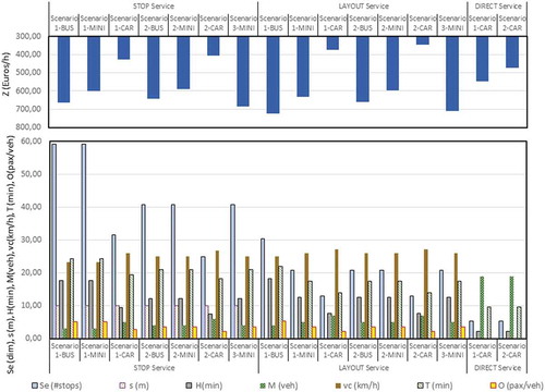
If we focus on electric cars (Scenario 2 CAR), STOP service is the cheapest (Z_a = 99 EUR/h) for the agency, although it is the worst from the user perspective (Z_u = 306 EUR/h, T= 18.31 min). In contrast, LAYOUT service presents a balance between user and operator costs: temporal costs decrease to 231 EUR/hour (T= 13.85 min) because the service visits the origins and destinations of users, although operating costs are increased by 17 Euros/hour. DIRECT service has a minimum value of user costs (Z_u = 160 EUR/h, T= 9.58 min) because the operational cost increases significantly (314 EUR/h). In this case, the distance traveled by the fleet in 1 hour (variable Q) is about 4 times the distance of bus services. DIRECT service needs 19 taxis to operate while only 6 and 7 cars are needed in STOP and LAYOUT services, respectively.

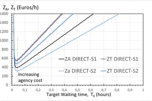
In Figures 3 and 4, we depict the variation of the total and operating cost (Z_T and Z_a) in LAYOUT and DIRECT service, respectively, when the temporal decision variable (headway or target waiting time) is steadily increased. The corresponding figure for STOP service has not depicted since it would be similar to LAYOUT service. An increment of these temporal decision variables implies worsening the service performance at the expenses of reducing the operating cost incurred by transit agency. It also highlights the existing trade-off between user and agency cost with regard to the decision variable of the system. However, this statement, in the case of DIRECT service, is only true when waiting times are lower than an optimal value. If we define taxi services operated at a waiting time T₀ higher than this threshold, the analytical model present inconsistencies, since more vehicles are needed and taxi performance is not improved. In the case of LAYOUT service, the system may not fulfill the vehicle capacity constraint when headways are increased.

Figure 3. Variation of total and agency cost with regard to target headway in LAYOUT service

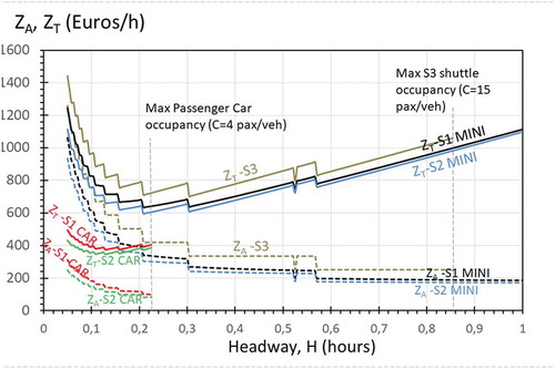
Figure 4. Variation of total and agency cost with regard to target waiting time in DIRECT service

This fact is especially important when passenger cars are operating the system since the maximal allowable headway turns to be H= 0.223 hours. In Figure 5, the agency and user variables are plotted with regard to the time headway H only for the LAYOUT service in Scenario 2 CAR, in the domain where the occupancy must be O≤ 4 pax/veh.

Figure 5. Variation of cost and performance metrics with regard to target headway in LAYOUT service

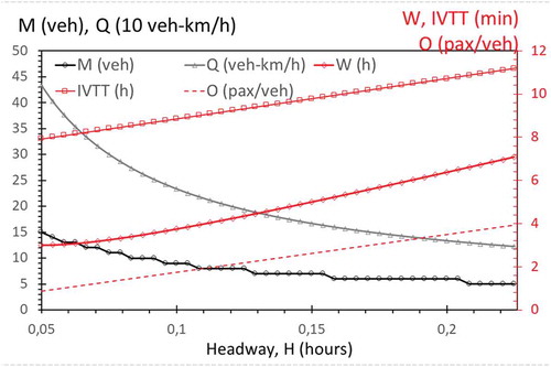
Finally, the agency cost per trip in LAYOUT and DIRECT services for different vehicle technologies is depicted in Figure 6 for the same domain of headway, as in Figures 3–4. We have also plotted the horizontal lines corresponding to a fare box recovery ratio $\eta$=1 in LAYOUT and DIRECT service. If unit agency cost is higher than this ratio, it means that the service is not economically feasible, given the current transport fare. Hence, the vast majority of scenarios of LAYOUT service are not profitable in the whole domain of H, they would be subsidized by the administration. Only the agency costs of Scenario 2, operated by cars, are lower than the agency incomes in a narrow domain of headways (0.15 < H< 0.23 hours). In the case of taxis, the unit agency cost is significantly lower than the expected average fare per trip for a wide range of T₀. This domain also includes the optimal value T₀*.

Figure 6. Variation of unit agency cost (z_p) with regard to target headway (LAYOUT service) or target maximal waiting time (DIRECT service)

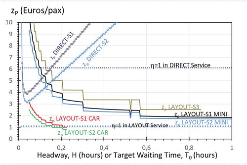
It can be noticed from Figure 3 that the total cost function remains quite stable around the minimum in LAYOUT and STOP services. Even if transit agencies design the system with suboptimal headways (near to the optimal), the extra cost that they may incur is small. In this sense, the enumeration of the headway variable presented in Section 2 can be calculated in $\mathrm{\Delta }H$ intervals of ½ or 1 minute. This statement is not true for DIRECT service, where the total cost function grows around itsoptimal value . In that case, direct services (taxis) based on dispatching centers may be designed ensuring a minimal waiting time of 1–2 minutes.

Sensitivity analysis with regard to the demand density

The results presented in Section 3.1 are calculated for a low level of on-demand trip densities. However, this section is aimed at analyzing the variation of the total and agency cost of the system when the demand density is increased for all on-demand services, ${\lambda }_d\in \left(1;660\right)$ pax/km²-h.

Eventually, the variation of the total and agency cost of the system when the demand density is increased for all on-demand services is depicted in Figures 7 and 8, respectively. Electric powertrains (Scenario 2) are always more cost efficient than diesel counterparts (Scenario 1). The crucial driver to minimize the total cost of the system in Figure 7 is the fleet size. The best solution is obtained when the smallest vehicle typology for each demand domain is deployed (passenger cars). For demand densities 3≤ λ_d≤92 pax/km²-h, it can be seen that LAYOUT service operated by electric cars (Scenario 2) minimizes the total cost (user and agency cost), followed by STOP service operated by electric cars and, in the third position, taxis. This is because the vehicles in STOP and LAYOUT service can be used by more than one passenger per trip. Nevertheless, since the former services present a maximal headway H_max = 3 min, they would exceed the vehicle capacity for demand densities higher than λ_d>92 pax/km²-h.

Figure 7. Unit total cost of the three services with regard to demand density

On the other hand, if the density domain ranges between 92< λ_d≤360 pax/km²-h, the electric taxi becomes the service with the minimal user and agency cost. In spite of being operated by cars of capacity C = 4 pax/veh, this service does not present any minimal headway as it happened in STOP and LAYOUT service. Therefore, the service can fulfill all customer calls even for large demand densities. The taxi service also gains applicability when the demand density is extremely low λ_d<1 pax/km²-h.

In crowded areas, STOP service is preferable when the demand density is λ_d>360 pax/km²-h. This is reasonable since we should deploy the service more similar to conventional systems with fixed routes and stops. In the 360< λ_d≤480 pax/km²-h subdomain, the operation with electric minibuses obtains the lowest value of Z.

It has to be noted that LAYOUT service is not competitive if vehicles of intermediate or huge size (minibuses or standard buses) operate the system. The deployment of these vehicles would only be justified if the vehicle occupancy would be remarkable. Nevertheless, under these conditions, any detour made by the vehicle to pick up or drop an additional passenger will increase the in-vehicle travel time of all passengers on board, worsening the corresponding monetary value of this service. This fact can be realized in Figure 7 by the increasing cost functions associated with this service (depicted by red series). Apart from that, Scenario 3 (autonomous vehicles) turns to be the worst option in the whole domain of demand densities. This fact is due to the unit cost parameters considered, that correspond to pre-marked prototypes. Assuming the current unit distance cost parameter c_d = 0.014 EUR/veh-km, autonomous minibuses must be rented below 197,500 EUR/year and 53,800 EUR/year in order to be competitive to the alternative electric minibus (Scenario 2) or electric cars (Scenario 3) respectively.

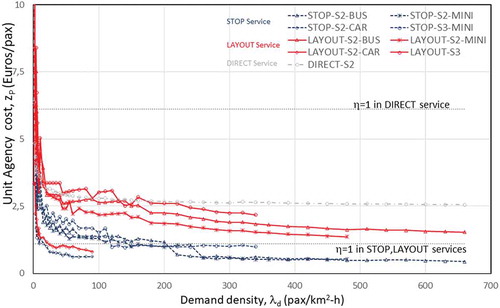
Finally, STOP service is also the most desired on-demand mobility option from the transit agency perspective in the whole demand domain considered, since the z_p cost component is minimized (see Figure 8). The size of the vehicle should be adapted to the expected ridership, using cars, minibuses, and buses for small, intermediate, and huge demand densities, respectively. The second-best deployment is LAYOUT service. It is noticeable that, as compared to total cost functions, the agency cost associated with LAYOUT service implementations does not grow with regard to the demand density increments. Taxi systems (DIRECT service) is the most expensive, considering the agency cost component. This service can only be recommended from the total cost perspective due to travel time savings.

The current taxi fare structure applicable in Barcelona (IMET 2018) justifies positive profitability for DIRECT service in the overall density domain, with a stable farebox recovery ratio $\eta$=6.1/2.65 = 2.3. Nevertheless, in STOP service we can only obtain $\eta$ >1 in the domains 15< λ_d≤92 and λ_d>200 pax/km²-h. Therefore, this service will need subsidies or the increment of the average fare to guarantee the transit agency profitability.

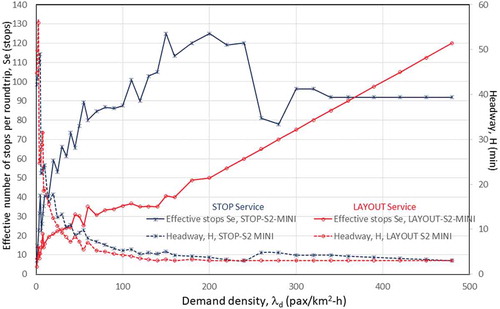
Eventually, Figure 9 depicts the evolution of the crucial variables that shape the spatial and temporal coverage in STOP and LAYOUT services. These variables are, respectively, the number of effective stops, Se, and the time-headway, H. For the sake of simplicity, we only plot the corresponding functions for minibuses in Scenario 2 (electric). It can be noticed that LAYOUT service is always operated at a lower headway than STOP service. This is due to the in-vehicle travel time caused by the detour incurred for any additional passenger. Therefore, the system tends to reduce the occupancy by deploying more frequent vehicle dispatches. For demand densities λ_d>270 pax/km²-h, LAYOUT service is operated at the minimal headway. As a result, the number of stops performed per roundtrip is also lower in LAYOUT service, compared to the corresponding metric in STOP service. However, the number of stops in STOP service is stabilized when a demand density threshold (around λ_d = 270 pax/km²-h) is achieved. Although we exceed this demand threshold, the system does not increase the number of stops. In case the system performs more stops in the same roundtrip, its commercial speed would drop, increasing the operating and user costs. With more information of on-board passengers, the system performance maybe even improved, optimizing the exact location of stops, with variable stop spacing (Medina-Tapia, Giesen, and Muñoz 2013; Zhang, Wang, and Meng 2019). On the contrary, in a LAYOUT service, the number of stops performed per roundtrip increases with regard to the demand density variable in the whole domain of analysis.

Figure 8. Unit agency cost of the three services with regard to demand density

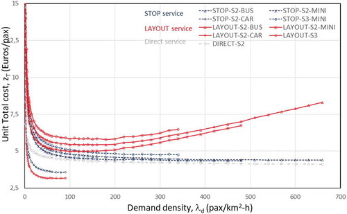
Figure 9. Number of effective stops (Se) and headway (H) with regard to demand density for STOP, and LAYOUT services operated by minibuses

Conclusions and future research

The economies of scale of transit modes (collective transportation services such as subways, tramways, high-performance buses) are based on high capacity systems that require significant initial investments. In this way, the average cost per trip of these systems usually presents a strictly decreasing behavior with regard to the demand density. This behavior is only partially followed by on-demand services with fixed routes and variable stop locations (STOP service). On the contrary, the economies of scale in the rest of the on-demand services are barely observed. The average cost per trip is only reduced when the demand density is low. Beyond a certain demand threshold, the unit total cost of flexible services is increased, as well as travel times. The route layout of these systems varies in each roundtrip and consequently, it is difficult to provide any kind of right of way. As a result, travel times may increase as the traffic density becomes higher. In addition to that, the service based on shared vehicle with variable route layout (LAYOUT service) would present increasing unit total costs with regard to demand. This fact is due to the detour incurred by the vehicle to serve any new customer. When the occupancy becomes larger in high demand domains, the extra travel time is penalized by more onboard passengers. This fact is also discussed in Wang, Dessouky, and Ordonez (2016) for ridesharing systems. More detours per vehicle should be only performed if HOV lanes and other priority measures ensure that ridesharing travel times are time-competitive to conventional passenger cars (with no priority). Therefore, the implementation of on-demand services with somewhat flexible design has the direct consequence of reducing the economies of scale of the transportation system and constraining the reduction of the average cost per user.

The results in the site under analysis demonstrate that each modality of flexible service is only efficient for a certain demand domain. For extremely low demand services (λ_d≤1 pax/km²-h), taxi systems become the desired flexible option over other services since there is no option to consolidate multiple trips in the same vehicle. However, when the probability of sharing trips with the same vehicle is increased, the LAYOUT service is more suitable. This behavior is maintained until the vehicle capacity operating the LAYOUT service is exceeded, which happens with low demand densities (3≤ λ_d≤92 pax/km²-h in our analysis). For intermediate demands above the former domain, taxi systems (DIRECT service) turn to be the most cost-efficient option. Finally, in high demand domains (λ_d>360 pax/km²-h in our analysis), STOP service, which presents less flexibility, is recommended. The implementation of a STOP service should start deploying minibuses of intermediate capacity. As the demand becomes even larger and we exceed the vehicle capacity, standard buses are required to allocate all potential passengers. Therefore, as the unit vehicle costs clearly depend on the vehicle size, transit agencies must adapt the fleet dimensions to the expected demand captured by each service.

The electric powertrains (Scenario 2) always outperform diesel-powered engine vehicles (Scenario 1) due to the lesser unit distance cost parameter. Nevertheless, in our analysis, we did not consider the capital cost associated with the charging infrastructure and the renovation of batteries after their lifetime. The autonomous vehicle technology (Scenario 3) is still never justified due to the vehicle depreciation cost. Future studies may estimate in more depth the infrastructure, battery, and autonomous vehicle depreciation cost, once these technologies will become more mature and the cost variability will have been reduced.

The model is capable of estimating the unit operating cost per passenger, (z_P), for each mode of service. This variable has resulted to be the main metric for financing the system and achieve an economically sustainable relationship among stakeholders. Based on this variable, decision-makers should define the fare structure to be implemented in order to have an adequate fare box recovery ratio parameter. In general, STOP and LAYOUT services have a decreasing unit cost of operation with demand. When operated by cars, they present unit agency cost around 0.9 EUR/trips, lower than the current fare ($\eta$>1). STOP service is also economically sustainable for large demand densities when the unit agency cost of buses is around z_P = 0.5 EUR/trip. In contrast, DIRECT services based on a taxi dispatching center always have a unit operation cost higher than 2.5 EUR/trip in the same range of demand. However, the service is profitable due to the different taxi fare structure.

Acknowledgments

The first and last authors thank AMTU (public entity Association of Municipalities with Urban Transportation) that supported this research under the contract C-11523 “Flexitransport” with our University Barcelona TECH. The contribution of the third author has been supported by the Chilean Scientific Research Agency (CONICYT), under the grant PFCHA/BCH No. 72160291.

Disclosure statement

No potential conflict of interest was reported by the authors.

Additional information

Funding

This work was supported by the Chilean Scientific Research Agency (CONICYT), [PFCHA/BCH No. 72160291]; AMTU [C-11523].

Appendix 1.

Glossary of terms and Nomenclature

Decision variables:

$H$time headway for STOP and LAYOUT services [h]

$T_0$maximal user’s waiting time for DIRECT service [h]

$s$stop spacing for STOP service [km]

Dependent variables:

$M$number of vehicles needed (fleet size) [veh-h/h]

$Q$distance traveled by the fleet in 1 hour of serv. [veh-km/h]

$A$ expected passenger access time [h]

$W$ expected passenger waiting time [h]

$IVTT$ expected in-vehicle travel time [h]

$O$on-demand vehicle occupancy [pax/veh]

$z_p$mean cost of a trip [EUR/pax]

$Z$ total cost of the system per hour [EUR/h]

$Z_A$ cost incurred by transit agency in 1 hour of service [EUR/h]

$Z_U$ cost incurred by users in 1 hour of service [EUR/h]

Parameters:

$R$area of urban region [km²]

$L$length of rectangular urban region [km]

$w$width of rectangular urban region [km]

${\lambda }_d$demand density of on-demand users [pax/h-km²]

$v_w$walking speed [km/h]

$v$cruising speed of vehicles [km/h]

$a$ acceleration [km/h²]

$l$longitudinal trip length of a user [km]

$\mathrm{\Delta }b$distance between streets [km]

Cbus capacity [pax/veh]

$\tau { }^{\mathrm{\prime }}$alighting and boarding time per user [sec/pax]

$H_{min}$ minimum headway [h]

$s_{min}$ minimum stop spacing in STOP service [km]

$s_H^2$variance of headway in STOP and LAYOUT services[h]

$t_{\theta }$payment time in DIRECT service [h/service]

$t_a$service assignment time by taxi control center [h/service]

Cost parameters:

$c_d$,$c_t$ unit operating cost per kilometer [EUR/veh-km], unit operating cost per hour [EUR/veh-h], respectively

${\beta }_T$perceived value of travel time [EUR/h-pax]

$\theta$, ${\theta }_{km}$ fare of the bus in STOP and LAYOUT service [EUR], distance-based fare in DIRECT service [EUR/km], respectively

$\mathrm{\Phi }$flag drop fare [EUR/service]

ηratio of the average fare income of an average trip and the operating cost of this trip [dimensionless]

References

- Ansari, S., M. Başdere, X. Li, Y. Ouyang, and K. Smilowitz. 2018. “Advancements in Continuous Approximation Models for Logistics and Transportation Systems: 1996–2016.” Transportation Research Part B 107: 229–252. doi:10.1016/j.trb.2017.09.019.
- Askari, S., F. Peiravian, N. Tilahun, and M. Y. Baseri. 2020. “Determinants of Users’ Perceived Taxi Service Quality in the Context of a Developing Country.” Transportation Letters. doi:10.1080/19427867.2020.1714844.
- ATM. (2018). Dades Bàsiques Del Sistema. [Accessed 20th March 2019]. https://www.atm.cat/web/ca/observatori/dades-basiques-del-sistema.php
- Bansal, P., Y. Liu, R. Daziano, and S. Samaranayake. 2019. “Impact of Discerning Reliability Preferences of Riders on the Demand for Mobility-on-demand Services.” Transportation Letters. doi:10.1080/19427867.2019.1691298.
- Cuevas, V., M. Estrada, and J. M. Salanova. 2016. “Management of On-demand Transport Services at a Urban Context. Barcelona Case Study.” Transportation Research Procedia 13: 155–165.
- Daganzo, C. F. 1978. “An Approximate Analytic Model of Many-to-many Demand Responsive Transportation Systems.” Transportation Research 12 (5): 325–333.
- Daganzo, C. F. 1984. “The Length of Tours in Zones of Different Shapes.” Transportation Research Part B 18 (2): 135–145. doi:10.1016/0191-2615(84)90027-4.
- Daganzo, C. F. 2010. Public Transportation Systems: Basic Principles of System Design, Operations Planning and Real-time Control. Berkeley: Institute of Transportation Studies, University of California.
- Dell’Olio, L., A. Ibeas, and P. Cecin. 2011. “The Quality of Service Desired by Public Transport Users.” Transport Policy 18 (1): 217–227. doi:10.1016/j.tranpol.2010.08.005.
- El Esawey, M., and T. Sayed. 2011. “Using Buses as Probes for Neighbor Links Travel Time Estimation in an Urban Network.” Transportation Letters 3 (4): 279–292. doi:10.3328/TL.2011.03.04.279-292.
- Estrada, M., and F. Robusté (2018). Memòria Executiva Del Model D’operació Dels Serveis De FLEXITRANSPORT. AMTU 2018. Working paper. BIT. Barcelona Innovation in Transport. [Accessed 20th June 2019]. https://bit.upc.edu/en/recent-projects
- Estrada, M., and M. Roca-Riu. 2017. “Stakeholder’s Profitability of Carrier-led Consolidation Strategies in Urban Goods Distribution.” Transportation Research Part B 104: 165–188. doi:10.1016/j.tre.2017.06.009.
- Estrada, M., M. Roca-Riu, H. Badia, F. Robusté, and C. F. Daganzo. 2011. “Design and Implementation of Efficient Transit Networks: Procedure, Case Study and Validity Test.” Transportation Research Part A: Policy and Practice 45 (9): 935–950.
- Hawkins, A. J. (2019). Ford’s On-demand Bus Service Chariot Is Going Out of Business. The Verge. On-line magazine. [Accessed 30th June 2019]. https://www.theverge.com/2019/1/10/18177378/chariot-out-of-business-shuttle-microtransit-ford
- HSL-Helsinki Regional Transport Authority. (2016). Kutsuplus – Final Report.
- IMET(2015). Observatori Del Taxi. Document Annual (In Catalan). Center for Innovation in Transport. [Accessed 23rd September 2017]. http://www.cenit.es/
- IMET (2018). Tarifes del taxi 2018. [Accessed 20th September 2018]. https://taxi.amb.cat/es/usuari/tarifes
- Kim, M., P. Schonfeld, and E. Kim. 2018. “Switching Service Types for Multi-region Bus Systems.” Transport Planning and Technology 41: 618–643.
- Liu, J., S. Jones, and E. K. Adanu. 2019. “Challenging Human Driver Taxis with Shared Autonomous Vehicles: A Case Study of Chicago.” Transportation Letters. doi:10.1080/19427867.2019.1694202.
- Medina-Tapia, M., R. Giesen, and J. C. Muñoz. 2013. “Model for the Optimal Location of Bus Stops and Its Application to a Public Transport Corridor in Santiago, Chile.” Journal of the Transportation Research Record 2352 (84–93). doi:10.3141/2352-10.
- Nissan. (2019) eNV-200 Nvalia Feature Template. [Accessed 03th November 2019]. https://www.nissan.es/vehiculos/nuevos-vehiculos/e-nv200-evalia.html
- Nourbakhsh, S. M., and Y. Ouyang. 2012. A Structured Flexible Transit System for Low Demand Areas.” In Transportation Research Part B, 204–216. Vol. 46.
- Ojo, T. K. 2019. “Quality of Public Transport Service: An Integrative Review and Research Agenda.” Transportation Letters 11 (2): 104–116. doi:10.1080/19427867.2017.1283835.
- Papanikolaou, A., and S. Basbas (2020). “Analytical Models for Comparing Demand Responsive Transport with Bus Services in Low Demand Interurban Areas.” Transportation Letters. doi:10.1080/19427867.2020.1716474.
- Piccioni, C., A. Musso, and U. Guida (2018). Training Material for University Workshops. Deliverable N°42.6. Zero Emission Urban Bus System Project. Seventh Framework Programme for Directorate General Mobility & Transport. European Commission. [Accessed 16th October 2019]. https://zeeus.eu/
- Rogers, G. (2017). Cities Now Exploring Autonomous Buses – But Is It Worth It? ENO Center of Transportation. [Accessed 27th September 2019]. https://www.enotrans.org/article/cities-now-exploring-autonomous-buses-worth/
- Salanova, J. M., and M. Estrada. 2018. “Modeling and Comparison of Taxi Operational Modes: Case Study in Barcelona.” Transportation Research Procedia 33: 59–66.
- Salanova, J. M., M. Estrada, G. Aifadopoulou, and E. Mitsakis. 2011. “A Review of the Modeling of Taxi Services.” Procedia-Social and Behavioral Sciences 20: 150–161.
- Taylor, B. D., and C. N. Y. Fink. 2013. “Explaining Transit Ridership: What Has the Evidence Shown?” Transportation Letters 5 (1): 15–26. doi:10.1179/1942786712z.0000000003.
- TMB. 2019. Total Cost of Ownership of Diesel, Hybrid and Electric Vehicles in Barcelona. Transports Metropolitans de Barcelona. Personal communication.
- Wang, X., M. Dessouky, and F. Ordonez. 2016. “A Pick-up and Delivery Problem for Ridesharing considering Congestion.” Transportation Letters 8 (5): 259–269. doi:10.1179/1942787515Y.0000000023.
- Zhang, J., D. Z. W. Wang, and M. Meng. 2019. “Optimization of Bus Stop Spacing for On-demand Public Bus Service.” Transportation Letters. doi:10.1080/19427867.2019.1590677.