Representing travel cost variation in large-scale models of long-distance passenger transport

ABSTRACT

In this paper, we show that cost variation for long-distance travel is often substantial and we discuss why it is likely to increase further in the future. Thus, the current practice in large-scale models, to set one single travel cost for a combination of origin, destination, mode, and purpose, has potential for improvement. To tackle this issue, we develop ways of accounting for cost variation in model estimation and forecasting. For public transport, two approaches are proposed. The first method focusses on improving the average fare, whereas the second approach incorporates a submodel for choice of fare alternative within a demand model structure. Only the second method is consistent with random utility theory. For car, cost variation is related to long run decisions such as car type choice. Handling car cost variation therefore implies considering car type choice. This long-term choice can be considered using a car fleet model.

KEYWORDS:

• Long-distance
• passenger transport
• travel cost
• travel fare
• large-scale model
• level of service data

Introduction

Large-scale transport models of long-distance¹ passenger transport are often used in cost-benefit calculations of infrastructure investments or policy implementations. One common application of such a model is to investigate the costs and benefits of building high-speed rail (Cambridge Systematics 2016; WSP 2011). The electric vehicle market is developing (Liu and Lin 2017; Jensen et al. 2017) and thus another application, likely to be more common in the near future, is to analyze the effects of electrification of the car fleet on long-distance travel. So far, analyses have mainly focussed on how electrification of the car fleet affects network design, i.e. where it is most beneficial to expand road capacity (Duell, Gardner, and Travis Waller 2018).

Both high-speed rail and electric cars form new cost alternatives for future long-distance travel. One core feature of large-scale transport models is therefore the way travel costs are represented in the model. For public transport (PT) modes such as rail, air, and long-distance bus, this refers to the representation of fares, whereas for car this refers to the representation of fuel and other operational costs in the model. More focus and scientific effort have traditionally been put on the demand modeling side, i.e. the estimation of behavioral parameters for mode and/or destination choice (Rohr et al. 2013; Moeckel, Fussell, and Donnelly 2015; Cheng et al. 2020). This is unfortunate, for example since deficiencies in cost data will also affect the cost parameter estimates, and in turn the value of travel time.

Often in large-scale modeling of PT cost, a single average fare is used for one combination of origin, destination, mode, and trip purpose (typically private or business). Sometimes the fare implemented in the model differs also by person type (e.g. commuters might be assigned season tickets). However, since aggregate figures for revenue and demand are rarely available to model developers (typically for reasons of commercial confidentiality), these average fares are usually based on ticket prices. The use of average fares may lead to counter-intuitive results since an improvement in the offer may lead to an overall decrease in the average PT utility if enough people change alternative. An example could be a reduction in the first-class fare, when the overall average price could increase, if there is a substantial increase in first-class travel. Another example could be when there is, for a given journey, one fast and one slow train service and a higher fare applies to the faster service. Then if the fare for the faster service is reduced somewhat, but not to the level of the slower service, some more travelers will use the fast service. What happens to the average fare in these cases? Those who were already using the premium service will pay less, but those who switch will pay more, and it is quite possible that the average fare will increase. Since no other aspect of the service has changed, this will imply that the overall rail service is less attractive, and a large-scale model will predict a switch away from train travel. The reason for the outcome of both examples is that the average fare is not consistent with random utility theory, on which the models are based and by which travelers are assumed to choose the alternative they perceive to give the best service, based on their own preferences.

Long-distance models that include submodels of the choice of different travel fares are scarce. Models exist, such as PRAISE in the UK (Whelan and Johnson 2004), which do model this choice, but they have a much more restricted scope compared to national large-scale travel models. However, large variation exists in travel costs both for PT modes and for car. Dynamic pricing strategies have increased, and rail and air operators often use revenue management strategies to adjust fares to actual demand and customer heterogeneity (Hetrakul and Cirillo 2015). The opening of the rail market for competition between different operators has also had an effect on ticket prices, for example in Sweden (Vigren 2017).

For car, the introduction of electric vehicles will likely increase travel cost variation further from a situation already differentiated by differences in car size, fuel type and fuel efficiency. The appropriate cost of driving a car that should be entered into model estimations or applications is not easy to state simply. Among the issues that need to be considered are:

• to what extent the ownership costs, i.e. the costs that are incurred whether the car is driven (e.g. most of the depreciation and insurance costs), should be included;

• how choices made by the owner or driver, such as the type of car or fuel and the driving style (e.g. speed choice), need to be considered;

• how taxation is accounted;

• how compensation in particular, by an employer, is included.

A useful text and recommendations on these issues can be found in the UK government’s Transport Analysis Guidance, called TAG or WebTAG (Department for Transport 2019). This approach is based on an attempt to calculate the marginal cost per kilometer to the owner or driver. The cost is based on a very detailed calculation of fuel consumption per kilometer which is intended to be an average for the UK vehicle fleet of vehicle efficiency and fuel type; forecasts of changes in efficiency and fuel type are also given. The WebTAG methodology for calculating car driving costs is used in many large-scale models for example, models for Manchester (RAND Europe 2013) and West Midlands (RAND Europe 2014). The method used in the Swedish long-distance model is similar to WebTAG with a detailed calculation of fuel consumption per kilometer, which is intended to be an average for the Swedish vehicle fleet (Trafikverket 2020). One difference is that car costs for business trips are assumed to be equal to those for private trips in the Swedish model, whereas this is not the case in the UK guidelines.

In this paper, we show that travel cost variation for contemporary domestic long-distance travel is substantial and discuss why it is likely to increase further in the future. Furthermore, we suggest several ways of accounting for public transport and car cost variation in model estimation and forecasting.

Example of contemporary travel cost variation for long-distance trips

Overview of long-distance travel in Sweden

Context

Sweden is a geographically extended country with about 1570 km from the southernmost to the northernmost point. Domestic long-distance travel is therefore quite common and has also been reinforced by a strong urbanization trend in past decades, spreading family generations over the country. The Swedish travel survey from 2011–2016 shows that as much as 74% of long-distance travel is private trips with varying purposes such as visiting family and friends, whereas only 14% are business trips (Berglund and Kristoffersson 2020). The most common travel modes for domestic long-distance travel within Sweden are car (73%), train (16%), air (5%), and long-distance bus (4.5%). Modal shares depend a lot on trip purpose, e.g. with train and air shares being substantially larger for business trips.

In many ways, Sweden is typical of European countries, so that the considerable diversity in travel costs and the discussion on how to account for this diversity is likely to be applicable also to other countries. Of course, discussion related to air travel is not relevant for smaller countries where domestic travel is not conducted by air.

Public transport

The data set used was collected during spring 2010 in a travel survey related to high-speed rail modeling (WSP 2011). Data were collected onboard for trains and at departure gates for air. The response rate was estimated to be about 75% on both modes. The survey responses included information about the current trip used in this project including origin and destination, the fare for the current trip leg, and questions about socio-economic background.

(Figure 1) shows that there is substantial travel cost variation for long-distance public transport even when fares are segmented by mode, OD pair and route. Fare distributions are segmented by the modes train and air, the OD pairs Stockholm-Gothenburg and Stockholm-Malmö (the two main OD-pairs for long-distance travel in Sweden, since they connect the three largest cities in Sweden), and the routes Arlanda-Gothenburg, Arlanda-Malmö, Bromma-Gothenburg, and Bromma-Malmö (dividing air travel from Stockholm between the two main airports Arlanda and Bromma).

Figure 1. Cumulative fare distributions within each mode (train or air), OD pair (Stockholm-Gothenburg and Stockholm-Malmö) and route (separating Bromma Airport (Bro) from Arlanda Airport (ARN)). Travel costs are given in SEK.²

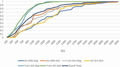
The fare distributions for the two train OD pairs are similar, one reason being that the same operator runs the service. The distributions are also not as wide as for air, as train tickets are cheaper in general.

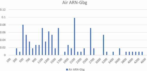
(Figure 2) shows the distribution of ticket prices for the air route Stockholm-Arlanda to Gothenburg, to better show the frequency of each fare class. The average fare is 1638 SEK, but the fare variation is large, as shown in the figure.

Figure 2. Distribution of ticket prices for air travel between Arlanda in Stockholm (ARN) and Gothenburg (Gbg).

Car

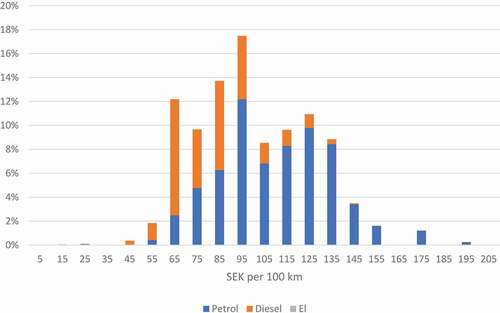
Somewhat more surprisingly, there is considerable variation also in car travel costs, see (Figure 3). Calculations are based on data from the Swedish car register containing fuel consumption for cars from years 2000–2014. The fuel consumption database reflects the passenger car fleet composition in early January 2015. The number of vehicles in the database includes 3 395,000 active cars registered in the 2000–2014 period. There is no fuel consumption information in the car register about cars with model year earlier than 2000. For each car in the database, fuel consumption per 100 km is multiplied by the fuel cost for each fuel type (petrol, diesel, and electricity) as of 2014, see (Table 1). The reader should keep in mind that petrol and diesel prices vary, which obviously may have an impact on the cost distribution. However, the correlation between petrol and diesel prices is very high, so this would affect the distribution mean rather than the variance. The price of electricity of 1.1 SEK/kWh in (Table 1) is calculated based on the assumption that the electric cars are charged at home. For long-distance travel, however, charging often needs to be done at public charging stations, where prices are much higher, up to 3 times higher than for home charging. For plug-in hybrids, range is quite important, as it also affects fuel type. The electric range for plug-in hybrids is often less than 50 km, implying that longer distance trips mostly will use petrol rather than electricity. Petrol consumption for plug-in hybrids may be quite high in many cases.

Figure 3. Fuel cost distribution for Swedish cars of model year 2000–2014.

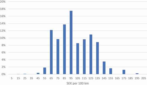
Table 1. Fuel costs in December 2014 in SEK per liter/kWh.

Petrol	Diesel	Electricity
14.32	14.19	1.1

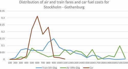
Car fuel costs vary less than air and train fares. Figure 4 shows the car fuel cost distribution for the OD pair Stockholm-Gothenburg, as well as the train and air fare cost distributions for the same OD pair. The car fuel cost standard deviation is 0.26 of the car fuel cost mean, the train fare standard deviation is 0.53 of the train fare mean, and the air fare standard deviation is 0.6 of the air fare mean (the ARN-Gbg route). It should be kept in mind that other car cost variation (e.g.depreciation) is not considered and also that it is assumed that there is only one person in the car. In modeling, we would calculate a cost per person depending on the car occupancy, so larger party sizes lead to less variation in absolute terms.

Figure 4. Train fare and fuel cost distribution for cars with model year 2000–2014 for the trip Stockholm – Gothenburg.

So far, what has been discussed is variation in vehicle costs, but for business trips, car travel costs are often not equal to the vehicle costs. Business travelers are compensated for their car travel with reimbursement and the level of reimbursement varies a lot. WSP (2016) shows that the reimbursement for travelers who used their private car for a business trip in Sweden in 2015 varied between 13 and 44 SEK per 10 km. The typical reimbursement is SEK 18.50, which is at present the maximum amount allowed without having to pay a benefit tax, but about half of car users got more than this amount. Also, for company benefit car users, the compensation for fuel costs varied between 2 and 55 SEK per 10 km in 2015 (WSP 2016).

Explanatory factors for contemporary travel cost variation

Public transport

Analysis of the data shows that the remaining cost variation (after segmentation by mode, OD pair, and route) is partially explicable by ticket type, departure time in peak and income for air travel, and by ticket type, senior citizenship, and income for train travel, as shown in Tables 2and 3, respectively.

Table 2. Regression models of air traveler fares.^3.

	Model 1		Model 2		Model 3		Model 4
Variable	Parameter	t-value	Parameter	t-value	Parameter	t-value	Parameter	t-value
GenderW							−179.4	−1.9
Inc40+					271.8	2.9	222.9	2.3
Inc-20					−375.0	−2.3	−306.3	−1.8
Age 65+			−275.2	−1.2	−230.5	−1.0	−222.4	−1.0
Age-27			−195.2	−1.3	16.4	0.1	10.1	0.1
OPSAS	178.4	1.6	189.0	1.7	166.9	1.6	131.1	1.2
RouteSG	37.2	0.4	35.9	0.4	−15.4	−0.2	−18.5	−0.2
FullFlex	1021.4	7.0	975.9	6.5	832.5	5.6	806.1	5.4
Flex	680.7	5.2	623.2	4.6	528.1	3.9	541.1	4.1
FixEconomy	17.4	0.2	−22.6	−0.2	−88.4	−0.8	−85.6	−0.7
Peak	363.9	3.7	333.5	3.4	353.6	3.7	356.2	3.8
Intercept	678.1	5.8	764.3	6.0	750.4	5.7	856.8	6.0
r^2	0.36		0.37		0.42		0.43

Table 3. Regression models of train traveler fares.^3.

	Model 1		Model 2		Model 3		Model 4
Variable	Parameter	t-value	Parameter	t-value	Parameter	t-value	Parameter	t-value
GenderW							−64.2	−1.8
Inc40+					135.7	3.2	123.1	2.8
Inc-20					−160.8	−3.1	−146.9	−2.8
Age 65+			−138.4	−2.4	−112.8	−2.0	−125.8	−2.2
Age-27			−91.8	−1.9	−12.2	−0.2	−29.6	−0.6
ODSG	69.3	1.8	55.7	1.4	−6.1	−0.2	−8.8	−0.2
Class1	257.2	6.2	252.1	6.1	211.4	5.1	208.7	5.0
Peak	63.8	1.7	67.2	1.8	52.1	1.4	48.0	1.3
Intercept	572.1	15.4	612.3	15.4	646.3	15.5	688.4	14.4
r^2	0.13		0.15		0.20		0.20

Table 2 shows that the ticket-type variables (FullFlex and Flex, but not FixEconomy), as well as the departure time in peak variable (Peak), are significantly different from zero and give significant contributions to the fare paid. These effects also remain when additional variables are included. The route effect for Stockholm-Gothenburg (RouteSG), implemented as a dummy which is equal to one if the route is Arlanda-Gothenburg, and the operator effect included as a dummy for SAS as operator (OPSAS) are not significant. Using a confidence level of 95% for a two-sided test, age effects (Age 65+ and Age-27) are also not significant, but income effects are (Inc-20 and Inc40+). As can be expected, travelers with income less than 20,000 SEK per month choose cheaper tickets, and travelers with income more than 40,000 SEK per month choose more expensive tickets. The gender variable (GenderW), which is one if the traveler is female, is not as significant as the ticket type and departure time in peak variables. When introducing the gender variable, the low-income variable becomes insignificant, probably because of a correlation between income and gender among these travelers.

In Table 3, the corresponding regression models for train are shown. Table 3 shows that for train, the first-class ticket-type variable (Class1) is significantly different from zero, whereas the dummy for OD pair Stockholm-Gothenburg (ODSG) and the departure time in peak (Peak) variables are not. When age is added, the effect for the group 65+ (Age 65+) also turns out to be significant, whereas that for the group under 27 years (Age-27) does not. Income effects (Inc-20 and Inc40+) also appear as significant, while the gender effect (GenderW) is marginal. Furthermore, the lower r²-values for train compared to air indicate that it is more difficult to explain the variation in train fares.

Car

The analysis of fuel cost variation shows that the main explanatory factors for fuel cost variation are fuel type, fuel efficiency, and model year. These factors are correlated, as both fuel type and fuel efficiency are dependent on model year. Diesel cars have become more common in Sweden in recent years, and electricity is starting to gain ground. Furthermore, newer cars are in general more fuel efficient than older cars. These changes in the Swedish car fleet over the years are partly caused by a number of car fleet policy measures.

Figure 5 shows that Diesel cars are in general cheaper per 100 kilometers than Petrol cars. This is slightly due to difference in fuel cost per liter (see Table 1) but mainly due to Diesel cars being more fuel efficient. Electric cars are too few to give a visible effect in the figure, but they are cheaper than most Diesel and Petrol cars per 100 kilometers.

Figure 5. Fuel cost distribution for Swedish cars of model year 2000–2014 segmented by fuel type.

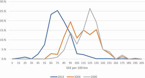
Figure 6 shows the fuel cost distribution for cars of model years 2000 (the first year in the data with fuel consumption information), 2006 (travel survey data for long distance model), and 2014 (national forecast base year), respectively. It is clear that the fuel cost distribution shifts to the left as years pass by, i.e. fuel costs decrease. This decrease in fuel costs is mainly driven by cars becoming more and more fuel efficient.

Figure 6. Fuel cost distribution for Swedish cars of model year 2000, 2006, and 2014, respectively.

Fuel cost can be expected to vary more in the future, because of the expected growth of electric vehicles, with considerably lower fuel costs compared to conventional vehicles. This growth will also be specifically driven by European and national climate policies. On the other hand, policy measures to ensure that marginal costs for car travel are internalized might be implemented in the future. These would likely be higher in congested areas (and during congested times) and would therefore be expected to affect urban travel to a higher degree than long-distance travel.

In addition to the detailed analysis of fuel costs above, we have also used official assumptions on distance driven depreciation costs (varying with car price) as well as on distance-dependent maintenance costs (fixed for all cars) to construct a distribution of total marginal car costs for new cars. The shape of the distribution changes, but the standard deviations are about the same when normalized. Also, as the cars get older, depreciation costs will be lower, and the total car cost distribution will come closer to the fuel cost distribution. This effect might, however, be damped somewhat by increasing distance-dependent maintenance costs of older cars.

Methods to account for cost variation in model estimation and forecasting

Public transport

The typical implementation of public transport costs in large-scale models is to use one average fare per mode, OD, and trip purpose. As indicated in the previous section, this approach does not capture existing cost variation. Moreover, the average-cost approach may even result in counter-intuitive results, as described in the introduction. We now describe two ways to better capture cost variation in model estimation and forecasting. Only the second approach is consistent with random utility theory.

Improving the average fare

A step that is very simple, in principle, is that the public transport average fare calculation can be improved by segmenting the fare into an increased number of fare categories and using data on the distribution of travelers over these fare categories.

The average fare for a traveler segment $k$ is calculated by

(1) $\overline{f_k}=\sum _j{p}_{jk}.f_{jk},$(1)

where$p_{jk}$ is the share of travelers in segment $k$ choosing fare category $j$ and

$f_{jk}$ is the fare these travelers pay for fare category $j$.

The improvement in cost representation using this method lies in the extended description of the travel fares that exist and the use of more detailed data on traveler distribution over these fare categories.

In some cases, analysts have access to aggregate statistics on the number of tickets of each category that have been sold in a given period and the revenue that these gave the operator. In other cases, these data are not available, perhaps for reasons of commercial confidentiality, and in these cases, the advertised ticket prices must be used. Using ticket prices can be difficult when these vary during the period, e.g. because of pricing algorithms for on-line sales.

The improvements given by increasing the number of traveler segments ($k$ in equation (1)(1) $\overline{f_k}=\sum _j{p}_{jk}.f_{jk},$(1) ) or of fare categories ($j$) are as follows: first, to improve the accuracy of calculation of the fares faced by specific travelers and second, to allow analysts to make forecasts of the effects of differential changes in fares. Even if there is no submodel to forecast changes in the distribution over fare categories, these can be substantial improvements in modeling accuracy. A key point is that the segmentation in the demand forecasting model should as far as possible match the categories of fare; this point needs particular consideration when aggregate data is available.

The implementation of segmentation over different fare categories requires path choice to be made for each fare category, using available public transport assignment software, to calculate level of service variables for that specific fare category. If the fare varies by route, then assignment needs to also take into account variation by person type, covering both the availability of some fare types to specific person types and the variation of the value of time in the population.

The distribution of travelers over fare categories may change in future, so that the average fare may change without any change in the prices of tickets. While the changes in the coming 20 years in the split over different public transport fare categories are not expected to be as large as the changes in split over different car fuel types, accurate forecasting also requires these shares to be forecast.

While simply improving the calculation of the average fare does not solve the theoretical problem of inconsistency with utility modeling (as explained in the next section), applying an increased segmentation so that the variation of fares within each segment is reduced will also reduce the impact of the theoretical problem.

Submodel for choice of fare alternative

In the introductory discussions, we noted that the use of a simple average fare is not consistent with the theory of individual utility maximization on which travel demand models are generally based. This can lead to paradoxical results, where an improved service can be assessed as giving lower utility, but even in less extreme cases the average fare will usually give incorrect changes in the overall attractiveness of public transport services. An alternative approach is then to take note of the utility basis of the modeling to derive a calculation method that is consistent with that basis.

In this second approach, we propose to use the logsum from a multi-fare choice model in mode-destination choice forecasting, to be consistent with random utility theory. It has long been known that, if choice for a set of alternatives is modeled using a logit model, then the only utility-consistent measure of composite utility for the set of alternatives is the logsum $L$ and is defined by

(2) $L=log(\sum _{j}exp{V}_j),$(2)

where$V_j$ is the utility of alternative $j$, usually a linear function of the fare and other attributes.

Usually, $V$ is calculated as the negative of a generalized cost.

The logsum is clearly not the same as the average utility, which is calculated by

(3) $\bar{V}=\sum _j{p}_j{V}_j.$(3)

To see how these are related, consider the logarithmic form of the logit model giving the log probability of choosing alternative $j$:

(4) $log{p}_j=V_j-log(\sum _{i}exp{V}_i)=V_j-L.$(4)

If we multiply equation (4)(4) $log{p}_j=V_j-log(\sum _{i}exp{V}_i)=V_j-L.$(4) by $p_j$ and add up over all the alternatives, we obtain, since the probabilities add up to 1,

(5) $\sum _j{p}_{j}log{p}_j=\sum _j{p}_j{V}_j-\sum _j{p}_{j}L=\bar{V}-L.$(5)

Reformulation of equation (5)(5) $\sum _j{p}_{j}log{p}_j=\sum _j{p}_j{V}_j-\sum _j{p}_{j}L=\bar{V}-L.$(5) leads to

(6) $L=\bar{V}-\sum _j{p}_{j}log{p}_j=\bar{V}+E.$(6)

That is, because all the log probabilities are negative, the logsum is larger than the average utility. The positive difference $\left(-\sum _j{p}_{j}log{p}_j\right)$ is referred to as ‘entropy’ $\left(E\right)$, by rough analogy with the use of that term in natural science and information theory (see Wilson (1970) and Shannon (1948) respectively).

The key feature of the logsum in the present context is that it responds correctly to fare changes, specifically, if we differentiate equation (2)(2) $L=log(\sum _{j}exp{V}_j),$(2) with respect to the fare of alternative $i$:

(7) $\frac{\mathrm{\partial }L}{\mathrm{\partial }{f}_i}=\frac{exp{V}_i}{\sum _{j}exp{V}_j}\frac{\mathrm{\partial }{V}_i}{\mathrm{\partial }{f}_i}=p_i{\beta }_f$(7)

where ${\beta }_f$ is the coefficient of the fare in the linear utility function $V_i$. This always has the correct (negative) sign and retains consistency with the utility theory underlying the model: an infinitesimal change in the fare of one alternative changes the overall utility $L$ proportionally to the choice probability of that alternative.

The differential of the logsum in equation (7)(7) $\frac{\mathrm{\partial }L}{\mathrm{\partial }{f}_i}=\frac{exp{V}_i}{\sum _{j}exp{V}_j}\frac{\mathrm{\partial }{V}_i}{\mathrm{\partial }{f}_i}=p_i{\beta }_f$(7) may be contrasted with the differential of the average fare which can be obtained from equation (3)(3) $\bar{V}=\sum _j{p}_j{V}_j.$(3)

$\frac{\mathrm{\partial }\bar{V}}{\mathrm{\partial }{f}_i}=\sum _j\left(\frac{\mathrm{\partial }{p}_j}{\mathrm{\partial }{V}_i}\frac{\mathrm{\partial }{V}_i}{\mathrm{\partial }{f}_i}{V}_j+p_j\frac{\mathrm{\partial }{V}_j}{\mathrm{\partial }{f}_i}\right)=\sum _j\left(p_i\left({\delta }_{ij}-p_j\right){\beta }_f{V}_j\right)+p_i{\beta }_f$

(8) $=p_i{\beta }_f(V_i-\bar{V}+1),$(8)

where ${\delta }_{ij}=1$ if $i=j$ and 0 otherwise.

Here we see that the correct result as in equation (7)(7) $\frac{\mathrm{\partial }L}{\mathrm{\partial }{f}_i}=\frac{exp{V}_i}{\sum _{j}exp{V}_j}\frac{\mathrm{\partial }{V}_i}{\mathrm{\partial }{f}_i}=p_i{\beta }_f$(7) is changed by the term $\left(V_i-\bar{V}\right)$. Thus, if the utility of $i$ is very bad relative to the average, to the extent that $\left(V_i-\bar{V}+1\right)<0$, there will be a change of sign. But, unless alternative, $i$ has utility exactly equal to the average, we do not obtain the correct result; the impact of changes will be less in absolute terms than the correct value if $\left(V_i-\bar{V}\right)<0$ and more than the correct value if $\left(V_i-\bar{V}\right)>0$.

The advantage of the formulation of equation (6)(6) $L=\bar{V}-\sum _j{p}_{j}log{p}_j=\bar{V}+E.$(6) is that we can now use the average fare (and average travel time, etc.) in calculating $\bar{V}$. In fact, the calculation of $\bar{V}$ is exactly what would be done if we were to use the averages for these variables as is done in existing travel demand forecasting models. All that must be done is to add the entropy to the utility.

In calculating entropy, we note that all that is required is the probabilities for each alternative. Some means must be found to forecast these, but this must be done in any case to calculate the average for the fare and other variables. This step is identical to the step of calculating traveler shares for the different fare categories in the averaging method described in the previous section.

The scale of equation (6)(6) $L=\bar{V}-\sum _j{p}_{j}log{p}_j=\bar{V}+E.$(6) , however, needs consideration. It would be reasonable to expect that the correlation of utilities between the fare alternatives for public transport would be higher than the correlation between public transport alternatives and other alternatives, e.g. other modes. This higher correlation has the effect that the scale of choice among ticket types, routes, etc., would be higher than the scale in the mode-destination choice model, i.e. the sensitivity of travelers’ choices to utility would be greater for within-mode switching than for between-mode switching. To deal with this issue, a scaling needs to be applied to the logsum derived from between-mode choice in order to use it in mode or destination choice models. This scaling is often designated by $\theta$, with $0<\theta \le 1$.

In extending an existing model to incorporate fare category choice, we can note that the coefficients within $\bar{V}$ have been estimated at mode-destination level, i.e. the scaling by $\theta$ is implicit within $\bar{V}$, so that what is required is to add $\theta E$ to the calculated mean utility. We would then arrive at a revised version of equation (6)(6) $L=\bar{V}-\sum _j{p}_{j}log{p}_j=\bar{V}+E.$(6) , giving the revised utility to use in the forecasting model:

(9) $\theta L={\bar{V}}^{\ast }+\theta E,$(9)

where ${\bar{V}}^{\ast }$ is the mean utility as currently used in the mode-destination modeling, with the scale defined for those choices.

Estimation of $\theta$ requires some additional investigation. Experience has shown that the impact of $E$ can be excessive, particularly when the number of alternatives changes. The extreme case is when a new alternative is introduced which has the same overall utility as a single existing alternative. The entropy changes from $0$ to $log2$, which is approximately 0.69, while the average utility does not change. In models of long-distance choice, where the coefficients are relatively small, the value 0.69 can represent many minutes of travel time, so that a careful calculation of $\theta$ is essential and the assumption that $\theta =1$ (as might be a naïve expectation) can cause difficulty. Ideally, data on choice between fare alternatives could be used to calibrate a value of $\theta$, but this is not always available, and a procedure based on judgment would then be used. For example, different values of $\theta$ could be tried and their impact on the elasticities indicated by the model; alternatively, values could be imported from another model.

We conclude that it is feasible to use this alternative logsum approach, to avoid basing the model entirely on averages of fare (and averages of other variables). However, this approach introduces some complications in programming the addition of entropy to the utility functions and in estimating the parameter $\theta$.

Car

As is discussed in section 0, there are expected to be considerable differences in marginal fuel cost between electric, hybrid, and internal combustion (i.e. petrol and diesel) cars. Determining an average car fuel cost therefore requires a good estimate of the split over fuel types, as well as forecasts of the costs of each fuel type. Moreover, the costs of electric cars may depend on tour lengths, particularly for long tours, which are the key focus of this study. These costs depend on technological developments and government policy, while the split further depends on traveler choices and the rate of incorporation of electric vehicles into the fleet. Car fuel cost variation is a different type of cost variation compared to public transport cost variation. For car, the variation is related to long run decisions like car type choice and employment location, whereas public transport cost variation is related to specific trips. Handling car fuel cost variation therefore implies considering car type choice and workplace choice rather than different options related to a specific trip.

It is easy to establish a base year car fuel cost distribution based on the Swedish car register (similar to the distributions shown in Figure 6). To be useful for forecasts, this distribution must be forecast as well. To do this, a car fleet model is needed. In 2006, such a model for Sweden was developed for the Swedish Road Administration. The Swedish car fleet model is a cohort-based model, where the base year car fleet is propagated year by year considering scrapping, car ownership level, and addition of new cars. The demand for a number of new cars is defined by the difference between the number of cars implied by the forecast car ownership level and the car fleet size after scrapping. The distribution of new cars by fuel type and fuel consumption is calculated using a discrete choice model. An earlier version of the model has been described in Beser Hugosson et al. (2016) and in Habibi et al. (2019). A recent version has been described in Engström, Algers, and Hugosson (2019). The model has also been used by Swedish planning authorities, the most recent application being for the Swedish Environmental Protection Agency 2017 (TPmod AB 2017).

The car fleet model output is currently quite aggregate but can easily be modified to also produce a distribution of car fuel cost per km, consistent with the car fleet input data. The distribution can then be used in two different ways. The simplest is of course to use the mean or the median of the distribution as car fuel cost in the mode-destination choice model. A more elaborate way would be to use the distribution as such, which would require the mode-destination choice model to be based on microsimulation (simulating behavior by individuals rather than groups of individuals) for example, by using Monte Carlo simulation. In a microsimulation setting, each individual would be assigned a specific car from the total distribution of cars. Currently, the car choice model operates at the national level, which means that no geographical variation is considered. Considering regional variation would require a regionalization of the model, which would also be necessary for analysis of geographically differentiated car fleet policies.

The variation in reimbursement for business trips can be accounted for when calculating car travel costs in the model. Currently, reimbursements are not explicitly considered at all in the Swedish long-distance model and are therefore implicitly accounted for in the cost coefficient of the model. It should be noted that this is not ideal from a model estimation point of view if the cost coefficient is constrained to be the same for all modes, which is the case for the business model. In such cases, it is important that all costs are included. One suggestion is to use the tax authority maximum amount allowed without having to pay a benefit tax for a certain share (from data) of the car users and an average for car users getting a different reimbursement. This method would apply both to travelers using their private car for business travel and to company benefit car users paying fuel costs privately, even though the shares and average reimbursements would differ between the two categories.

Conclusions

In this paper, it has been shown that travel costs for long-distance trips vary significantly for both car and public transport (train and air) for the Swedish case; the coefficient of variation is 53% for train travel, and for air travel, it is 60%. The main factors influencing the fares are ticket type, departure time and income for air travel, and ticket type, senior citizenship, and income for train travel. Given that the air and rail market have opened up for competition in many countries in Europe, Sweden is likely a representative case. Even though travel cost is one of the most important input data when using large-scale models to conduct cost-benefit analyses of major transport projects, travel cost, and especially travel cost variation, is inadequately represented in most large-scale systems of long-distance trips.

For large-scale transport modeling systems in Europe, we find that somewhat more effort has been put into the modeling of car cost variation compared to public transport cost variation, although the coefficient of variation is less, at 26%. In several cases, car fleet models are used to model the composition of different fuel types and fuel consumption levels in the national car fleet, both at present and for the forecast year. Furthermore, the calculation methodology is often well documented and easy to follow. However, there is room for some improvement also for car cost calculations. The detailed data from car fleet models already used could be utilized better. Given mode and destination choice models in which a synthetic population is used, the full car cost variation could be modeled by making draws from the car fleet and assigning one specific car to each car user in the synthetic population. However, one should remember that this ignores within-household choices concerning which vehicle to use from the household fleet for different activities (Angueira et al. 2019).

Cost modeling for public transport trips has even larger potential for improvement. Most large-scale models refer to unpublished reports when discussing the costs that are used for public transport long-distance travel. A more transparent process and documentation of public transport travel costs would be beneficial to the overall development of large-scale modeling. Furthermore, we show in this paper that the current practice of using one average fare per mode, OD pair and trip purpose, is not consistent with utility theory if several fare alternatives are available to the traveler, e.g. depending on service, route, or ticket category. In this case, an improvement in the offer to the traveler might lead to an overall decrease in the utility for that mode. In this paper, we show that this problem can be overcome by introducing a logit fare choice model and using the logsum from the fare choice model in the mode and destination choice model. We also show that this logsum is composed of the average fare plus a term called entropy, which is related to the switching of fare alternatives. When implementing such a fare choice model, one also needs to include a scaling factor for the entropy to account for correlation between similar alternatives, since travelers usually switch more easily between different fare alternatives, compared to changing mode or destination.

Disclosure statement

No potential conflict of interest was reported by the author(s).

Additional information

Funding

This work was conducted within the Primo project funded by the Swedish Transport Administration under Grant TRV 2019/11943; Swedish Transport Administration [TRV 2019/11943];

Notes

1. The exact definition of a long-distance tour varies among countries, where, e.g. 100 km is the cutoff distance in Sweden and 50 miles the cutoff in Great Britain. An important aspect of long-distance travel is that the available modes often differ compared to regional travel, with air, long-distance train and bus often being available for long-distance trips, whereas bicycle, walk, metro or tram are not options as main mode.

2. 10 SEK ≈ 1 EUR

3. Applying a two-sided test for the significance of the estimates, i.e. assuming that the sign of the coefficient is not known a priori, $p$ values will be obtained of$p=0.1$ for a t-value of 1.7 or more, $p=0.05$ for a t-value of 2.0 or more, $p=0.01$ for a t-value of 2.6 or more.

References

- Angueira, J., K. C. Konduri, V. Chakour, and N. Eluru. 2019. “Exploring the Relationship between Vehicle Type Choice and Distance Traveled: A Latent Segmentation Approach.” Transportation Letters 11 (3): 146–157. doi:10.1080/19427867.2017.1299346.
- Berglund, S., and I. Kristoffersson. 2020. “Anslutningsresor: En Deskriptiv Analys (Connection Trips: A Descriptive Analysis).” 3. Working Papers in TransportEconomics. https://www.diva-portal.org/smash/get/diva2:1416370/FULLTEXT01.pdf
- Cambridge Systematics. 2016. “California High-Speed Rail Ridership and Revenue Model” https://www.hsr.ca.gov/docs/about/ridership/CHSR_Ridership_and_Revenue_Model_BP_Model_V3_Model_Doc.pdf
- Cheng, L., X. Lai, X. Chen, S. Yang, J. De Vos, and F. Witlox. 2020. “Applying an Ensemble-Based Model to Travel Choice Behavior in Travel Demand Forecasting under Uncertainties.” Transportation Letters 12 (6): 375–385. doi:10.1080/19427867.2019.1603188.
- Department for Transport. 2019. “TAG UNIT A1.3 - User and Provider Impacts” https://assets.publishing.service.gov.uk/government/uploads/system/uploads/attachment_data/file/805260/tag-unit-a1-3-user-and-provider-impacts.pdf
- Duell, M., L. M. Gardner, and S. Travis Waller. 2018. “Policy Implications of Incorporating Distance Constrained Electric Vehicles into the Traffic Network Design Problem.” Transportation Letters 10 (3): 144–158. doi:10.1080/19427867.2016.1239306.
- Engström, E., S. Algers, and M. B. Hugosson. 2019. “The Choice of New Private and Benefit Cars Vs. Climate and Transportation Policy in Sweden.” Transportation Research Part D: Transport and Environment 69: 276–292. doi:10.1016/j.trd.2019.02.008.
- Habibi, S., M. B. Hugosson, P. Sundbergh, and S. Algers. 2019. “Car Fleet Policy Evaluation: The Case of Bonus-Malus Schemes in Sweden.” International Journal of Sustainable Transportation 13 (1): 51–64. doi:10.1080/15568318.2018.1437237.
- Hetrakul, P., and C. Cirillo. 2015. “Customer Heterogeneity in Revenue Management for Railway Services.” Journal of Revenue and Pricing Management 14 (1): 28–49. doi:10.1057/rpm.2014.27.
- Hugosson, B., S. A. Muriel, S. Habibi, and P. Sundbergh. 2016. “Evaluation of the Swedish Car Fleet Model Using Recent Applications.” Transport Policy 49: 30–40. doi:10.1016/j.tranpol.2016.03.010.
- Jensen, A. F., E. Cherchi, S. L. Mabit, and O. Juan de Dios. 2017. “Predicting the Potential Market for Electric Vehicles.” Transportation Science 51 (2): 427–440. doi:10.1287/trsc.2015.0659.
- Liu, C., and Z. Lin. 2017. “How Uncertain Is the Future of Electric Vehicle Market: Results from Monte Carlo Simulations Using a Nested Logit Model.” International Journal of Sustainable Transportation 11 (4): 237–247. doi:10.1080/15568318.2016.1248583.
- Moeckel, R., R. Fussell, and R. Donnelly. 2015. “Mode Choice Modeling for Long-Distance Travel.” Transportation Letters 7 (1): 35–46. doi:10.1179/1942787514Y.0000000031.
- RAND Europe. 2013. “Manchester Motorway Box - Post-Survey Research of Induced Traffic Effects” TR676. https://www.rand.org/pubs/technical_reports/TR676.html
- RAND Europe. 2014. “PRISM 2011 Base - Mode-Destination Model Estimation” RR186. https://www.rand.org/pubs/research_reports/RR186.html
- Rohr, C., J. Fox, A. Daly, B. Patruni, S. Patil, and F. Tsang. 2013. “Modeling Long-Distance Travel in Great Britain.” Transportation Research Record 2344 (1): 144–151. doi:10.3141/2344-16.
- Shannon, C. E. 1948. “A Mathematical Theory of Communication.” The Bell System Technical Journal 27 (3): 379–423. doi:10.1002/j.1538-7305.1948.tb01338.x.
- TPmod, A. B. 2017. “Bilparkens Utveckling 2017 –2030 Med Hänsyn till Nya Styrmedel - En Simuleringsstudie.” Report TPmod (in Swedish).
- Trafikverket. 2020. “PM Förutsättningarför Fordon, Drivmedel Och Körkostnader I Basprognos 2020” https://www.trafikverket.se/contentassets/19d85cfc691b4df3bff6c851d4097623/2020/pm-forutsattningar-fordon-drivmedel-och-korkostnader-basprognos-2020.pdf
- Vigren, A. 2017. “Competition in Swedish Passenger Railway: Entry in an Open Access Market and Its Effect on Prices.” Economics of Transportation 11: 49–59. doi:10.1016/j.ecotra.2017.10.005.
- Whelan, G., and D. Johnson. 2004. “Modelling the Impact of Alternative Fare Structures on Train Overcrowding.” International Journal of Transport Management 2 (1): 51–58. doi:10.1016/j.ijtm.2004.04.004.
- Wilson, A. G. 1970. Entropy in Urban and Regional Modelling. London, UK: Pion Press.
- WSP. 2011. “Höghastighetståg - Modellutveckling, Forskningsrapport (High Speed Train - Model Development, Research Report)” http://fudinfo.trafikverket.se/fudinfoexternwebb/Publikationer/Publikationer_001401_001500/Publikation_001404/HHT%20rapport_110622.pdf
- WSP. 2016. “Val Av Förmånsbil - Förmånsbeskattning, Företagspolicy Och Konsumentpreferenser” FUD-rapport. https://www.trafikverket.se/contentassets/773857bcf506430a880a79f76195a080/forskningsresultat/val_av_formansbil_formanbeskattning_foretagspolicy_och_konsumentpreferenser.pdf