Vehicle ownership models for a sharing economy with autonomous vehicle considerations

ABSTRACT

This study investigates the impacts of the sharing economy and vehicle automation on household vehicle ownership by considering the earning potential of household vehicles. While many studies have examined the impact of the sharing economy (namely ridesourcing) on vehicle ownership of ridesourcing customers, there is a gap in understanding its impact on vehicle ownership among ridesourcing suppliers. Data from an original survey are used to develop discrete choice models that evaluate the effects of earning potential, automation, and shared autonomous vehicle services on vehicle transaction decisions. The estimated models are applied to perform national-level simulations. It is found that, in comparison to a non-sharing economy context, individuals in the sharing economy tend to purchase more vehicles in times of income gain, and to preserve their fleets more readily in times of income loss. This study provides evidence that the sharing economy incentivizes some individuals to own more – not fewer – vehicles..

KEYWORDS:

• Vehicle ownership
• vehicle transaction
• sharing economy
• income generation
• autonomous vehicle
• ridesourcing
• discrete choice
• shared AV

Background

The sharing economy, in its various forms including ridesourcing and carsharing, is argued to reduce vehicle ownership from the perspective of treating individuals as the sources of travel demand (Botsman and Rogers 2010; Cervero, Golub, and Nee 2007). However, the sharing economy also enables individuals to be sources of transportation service supply. With ready connection of buyers and sellers in online marketplaces, vehicle owners can extend use of their vehicles beyond personal purposes to offering rides to and sharing vehicles with other people and using the vehicles to deliver food and other freight, to earn extra income. These new possibilities for income generation provide individuals with new incentives to own and keep vehicles, which could be further strengthened with the advent of vehicle automation, as doing the above income generating activities does not require the vehicle owner to be present in an autonomous vehicle (AV). Consequently, the tendency to own vehicles due to the sharing economy and vehicle automation may offset the argued effects of reduced vehicle ownership.

Existing research has already performed empirical investigations into the effects of sharing economy and vehicle automation on household vehicle ownership (HHVO). In terms of sharing economy, two of the most prominent demonstrations are ridesourcing and carsharing (e.g., Uber and Lyft). For ridesourcing, a systematic review of the relevant literature is conducted in Jin et al. (2018) who conclude that ridesourcing does not reduce HHVO, which is supported by the empirical evidence that ridesourcing draws largely from taxi and transit (Schaller 2017). On the other hand, carsharing is shown to reduce vehicle ownership among its users (Martin, Shaheen, and Lidicker 2010; Costain, Ardron, and Habib 2012). In terms of vehicle automation, it is argued that the need for individual vehicle ownership can be reduced as the travel demand of a household can be met with as few as one AV (Auld et al. 2018; Javanmardi, Auld, and Gurumurthy 2019). Moreover, a centralized AV fleet could accommodate travel demand from most or all individuals in a city, transforming mobility to a service or utility (Hughes 2018; Mitchell 2019). It is also expected that AV will gain a non-trivial market share in the coming decades. Many industrial and academic endeavors are made to project the market share of AVs and shared AVs (SAVs) in the future (Spieser et al. 2016; Fagnant and Kockelman 2014; Bischoff and Maciejewski 2016; Deloitte 2016; Chen, Kockelman, and Hanna 2016; Martinez and Viegas 2017; Heilig et al. 2017; Noruzoliaee, Zou, and Liu 2018; Gurumurthy, Kockelman, and Simoni 2019; Simoni et al. 2019).

Despite the above efforts, two important gaps remain. First, no existing studies have quantified the potential impacts of ridesourcing and carsharing on HHVO from the perspective of using owned vehicles to provide transportation services and generate income. Second, while some discussions briefly touch on income generation using owned AVs (Campbell 2018), no work has tried to quantify the implications of income earning using AVs for vehicle ownership. The objective of this paper, therefore, is to fill these gaps by conducting an empirical study to assess the impacts of sharing economy and vehicle automation on HHVO. The novelty of this study is twofold: 1) explicitly considering income earning while designing a series of experiments for vehicle transaction choice under different scenarios of income gain and loss, introduction of AV/SAV, and vehicle disposal in the presence of AV/SAV; 2) simulating the impacts of the sharing economy and vehicle automation on HHVO at the national level. The ability to predict changes in HHVO in response to the sharing economy and vehicle automation has not been adequately considered, but is critical for evaluating travel demand; assessing the impacts on road congestion, environment, and safety; and testing effectiveness of measures such as those related to technology platform development that may improve mobility, livability, or other desirable qualities.

Given that relevant data do not exist, in this paper we first conduct stated preference (SP) experiments to collect information on individuals’ vehicle transaction preferences with explicit recognition of earning possibilities using owned vehicles. The SP experiments encompass three circumstances: 1) considering income change in today’s sharing economy environment; 2) considering a future environment with three alternatives: buying a conventional vehicle (CV), buying an AV, or using a shared autonomous vehicle (SAV) service; and 3) considering vehicle disposal with AV/SAV. Using the SP data, discrete choice models are estimated to infer the impacts of earning potential on household vehicle transactions.

The estimated models are then employed along with National Household Travel Survey (NHTS) data from 2017 to simulate HHVO changes for the US, with the sharing economy and with both sharing economy and vehicle automation. A set of alternative models, which are developed using data collected prior to the advent of the sharing economy and vehicle automation, are also applied to the NHTS data to simulate a counterfactual estimate of HHVO changes without sharing economy and vehicle automation effects. Results provide new insights about how earning potential brought by the sharing economy and vehicle automation could affect vehicle ownership, and can inform economic and policy interventions to achieve reduced vehicle ownership or other desired mobility outcomes in the presence of the sharing economy and vehicle automation.

The remainder of this paper is organized as follows. Section 2 presents the data collection effort and salient descriptive statistics of the collected sample. Section 3 discusses the model estimation methodology and estimation results using the collected data. In Section 4, the estimated models are applied to NHTS data to simulate vehicle ownership changes at the national level. Finally, findings are summarized and directions for future research are suggested in Section 5.

Data collection and sample statistics

An original survey is conducted in this study. In total, 654 individuals are included in the survey.¹ Following the survey effort, removing responses with incomplete or inconsistent information leaves completed surveys from about 400 individuals for analysis.

The survey is conducted in three rounds. First, the survey is piloted online with a convenience sample of 199 friends, family and acquaintances of the authors. The pilot survey data are used to confirm that meaningful results can be obtained using the survey instrument. Then, an online survey of 245 students and staff recruited from the authors’ institution is conducted. The online survey is simple to administer but has the drawback of sampling only individuals who are affiliated with higher education. So, to ensure broader representation of viewpoints within the sample, an in-person survey of 210 visitors randomly recruited at Millennium Park in Chicago is also performed. The in-person data collection uses a paper survey. Appendix A shows an example of the paper version of the survey instrument.

The main feature of the survey is a series of SP experiments covering HHVO choice scenarios. Supporting information on sociodemographic characteristics and basic travel behavior of survey respondents is also collected.

The structure of the survey questionnaire is shown in Figure 1. Part 1 asks a series of questions about current travel habits – for example, frequency of travel using various modes such as driving, taking transit, and ridesourcing – and distance of home-to-work or home-to-school trips. Although land use is not included in the questions asked, the travel habits data collected here can implicitly reflect land use. In Part 2, information on household vehicle availability is collected. A household vehicle is described as one that is owned or leased by a household member and typically parked at home when not in use. Respondents are also asked if any of their vehicles are currently being used to generate income by a household member. Part 3 introduces three methods that are commonly used today to generate income with a household vehicle: ridesourcing, renting out a household vehicle, and food delivery. These methods are presented to survey respondents, who are then asked about their preferences. Although this part is not used for modeling or analysis in the paper, it helps survey respondents familiarize themselves with the vehicle transaction experimental context.

Figure 1. Structure of the survey.

Part 4 is the main body of the survey and it includes four SP choice experiments related to vehicle transactions, which are explained in detail in the rest of this section. In Part 5, respondents are asked about their sociodemographic characteristics such as household size, the number of workers, the number of children, and household income.

Choice experiments

Four stated preference (SP) choice experiments on vehicle transaction are administered. The first experiment examines the propensity of individuals for vehicle transaction with income generation (VT+IG) when an individual experiences an income increase. The experiment is conducted again, using an income loss scenario the second time. The third experiment considers a futuristic situation in which both CVs and AVs can be purchased. In addition, one has the option of using shared autonomous mobility. Vehicle ownership decisions in this futuristic situation thus involve not only income generation, but also the possibility of using (shared) autonomous vehicles. This experiment is labeled VT+IG+S/AV. The fourth experiment asks about vehicle disposal and is posed to respondents who choose an AV or SAV option earlier. The rest of this section describes the vehicle transaction experiments.

Choice experiments 1 and 2: vehicle transaction with income earning

In the first two choice experiments, survey respondents are asked about vehicle ownership in the context of the sharing economy, in which it is possible to use household-owned vehicles to earn income. On the other hand, as vehicle ownership is commonly influenced by income change, the vehicle ownership choices combined with income earning choices are presented in two choice experiments: one with an income gain, and the other with an income loss.

In choice experiment 1 (income gain), a job change leads to an income gain, which is randomly drawn from four possible values, or levels: $5,000, $10,000, $15,000, or $20,000. The new job will be located 15 miles away from home with no transit access. The respondent is asked to choose one out of three options: 1) buy a new vehicle and use the vehicle to generate income (termed ‘Buy & earn’); 2) buy a new vehicle but do not use the vehicle to generate income (termed ‘Buy & don’t earn’); and 3) neither, i.e., making no changes to the current household fleet (Figure 2). The intent of specifying the distance and transit accessibility is to create a situation where a car is effectively required for commute, so as to generate more instances for studying ‘Buy & earn’ vs. ‘Buy & don’t earn’ choices. It should be noted that while the experiment accomplishes this aim, considering the event of a job (and workplace location) change may limit the application possibilities for the estimated model. Future studies could consider exploring a wider range of events, such as a salary increase with no change in workplace location. It is assumed that respondents who select (3) would not use an existing vehicle to earn income. This assumption is based on the premise that in an income gain situation brought by a job change, the individual would likely have little reason to use an existing vehicle to earn additional income, unless s/he has access to more vehicles (which is not the case in (3)).

Figure 2. Options under choice experiments 1 and 2.

Choice experiment 2 (income loss) presents an economic downturn scenario that leads to a reduction in household income by 10%, 20%, or 30%. For a given respondent, the percentage reduction is randomly picked among these three levels. The respondent is asked to choose one also out of three options: 1) sell a vehicle (or end a lease) (termed ‘Sell’); 2) keep existing vehicles and use one of them to generate income (termed ‘Keep & earn’); and 3) neither. Similar to choice experiment 1, ‘neither’ means that the respondent makes no changes to her/his existing household fleet and s/he will not use an existing vehicle to earn income. Respondents from zero-vehicle households are not asked about an income loss scenario, as ‘Sell’ and ‘Keep & earn’ are not relevant options for them.

It should be noted that the choice sets in the two experiments are informed by the existing literature (e.g., Litman 2019) which supports positive elasticities of vehicle ownership with respect to an individual’s income. On the other hand, in times of an income loss, it might be possible for an individual to buy a vehicle to earn income with it. While this option is not included here, extensions of the present study could consider this ‘Buy & earn’ choice.

Choice experiment 3: vehicle ownership with S/AV

This choice experiment first presents the respondent with the same new job with income gain scenario (subsection 2.1.1) that was shown earlier to the respondent. Then, given this scenario, respondents are asked to choose one out of five options in a future environment where both AVs and CVs are available: 1) buy a CV; 2) buy an AV; 3) use SAV for work only; 4) use SAV for all purposes; and 5) none of the previous four. In the rest of the paper, these five options are termed as ‘CV-buy’, ‘AV-buy’, ‘AV-share work only’, ‘AV-share unrestricted’, and ‘None’, as shown in Table 1. In such an environment, an individual may buy a vehicle (either CV or AV). If buying an AV, the individual can also use the vehicle to earn income. Alternatively, an individual can choose to use SAVs for either the work commute only or unrestricted trip purposes. Unlike the previous two experiments, this experiment allows a respondent to consider oneself as either a provider of mobility service (by using one’s own vehicles to earn income) or a consumer of mobility service (by using SAVs). By doing so, the tradeoff between owning a vehicle motivated by income earning and using SAVs can be explicitly characterized.

Table 1. Vehicle owning/sharing choice alternatives, attributes, and attribute levels in the third SP choice experiment.

	CV-buy	AV-buy	AV-share work only	AV-share unrestricted	None
Down payment ($)	2,500,5,000	5,000,10,000
Monthly cost ($)	250, 500	500, 1,000	250, 500	500, 1,000
Monthly earning potential ($)		250, 500, 1,000
Avg. wait time (minutes)			5, 10, 15	5, 10, 15
Avg. percentage of shared rides			25%, 50%	25%, 50%
Avg. detour time when ride sharing occurs (minutes)			5, 10, 15	5, 10, 15

In Table 1, each column corresponds to one alternative, while each row represents one attribute. Each cell of the table shows the possible values, or levels, for the associated attribute and alternative. When an individual is surveyed, one level is selected randomly for each attribute from its set of possible levels. An empty cell means that the attribute is not relevant to an alternative. The first two alternatives, ‘CV-buy’ and ‘AV-buy’, involve a down payment as well as a monthly cost due to recurring payments, vehicle energy use, maintenance, insurance, etc. The ranges for CV down payments and monthly costs are determined based on the authors’ experience and previous research (Experian 2017; Edmunds 2020). For both down payment and monthly cost, AVs are expected to be more expensive than CVs (Noruzoliaee and Zou 2022). On the other hand, an AV can generate income without its owner being in the vehicle. When an AV is used to offer riding service to a customer, unlike current vehicle renting, the customer will not need to travel to the location of the vehicle. Instead, the AV will drive itself to pick up the customer.

Since multiple attributes are involved in this choice experiment, the idea of full factorial design, i.e., random numbers are drawn from the full factorial (Louviere et al. 2000), is pursued. The main benefit of using a full factorial design is that second- and even higher-order interactions between attributes that may be desirable for testing can be captured. While in some cases a full factorial utilization could lead to inefficient parameter estimation, in this study parameter estimate efficiency (which manifests itself by relatively small standard errors and large values for t-statistics) can still be achieved since the number of attributes and attribute levels included in our experiments is relatively small compared to the number of respondents.

Because of the self-driving feature, an individual may prefer to call an AV as a service when needed, rather than owning an AV. In fact, it has been argued that a significant part of future AVs will be used in a shared fashion (Fagnant and Kockelman 2014; Boesch, Ciari, and Axhausen 2016; Chen, Kockelman, and Hanna 2016;; Noruzoliaee and Zou 2022, to name a few). To reflect this, ‘AV-share work only’ and ‘AV-share unrestricted’ are provided as the third and the fourth alternatives. We conjecture that the probability of choosing these alternatives depends on not only the monthly cost of using SAV, but also quality of the riding service provided, characterized by three attributes: average wait time, average percentage of shared rides, and average detour time when ride sharing occurs. The two alternatives differ by the extent of using SAVs (for work only vs. for all purposes). The ranges for monthly cost for the two ‘AV-share’ alternatives are designed to be comparable with possible monthly pass cost in relatively expensive transit systems. For instance, travel by transit over any distance throughout the Chicago region requires a regional rail monthly pass for about $240 (Metra 2021) and an additional bus and urban rail pass for $105 for unlimited times (Chicago Transit Authority 2021); the additional bus and urban rail pass cost is $55 if urban transit is constrained to weekday peak periods (Metra 2021). The ranges for the three service attributes are determined based on the authors’ collective judgment. The percentage of solo vs. shared rides is an important determinant of ride quality for some passengers (Alonso-González et al. 2020).

Lastly, a fifth alternative, which is not doing any of the previous four, is introduced. This alternative is likely to be chosen when the travel needs of a respondent can be met by her/his existing household fleet and s/he is not interested in an autonomously driven vehicle.

Choice experiment 4: vehicle disposal with S/AV

In the future, travel needs of households that use AVs or SAVs may be met with fewer owned vehicles (Fagnant and Kockelman 2014; Auld et al. 2018). It is then reasonable to assume that some households may sell or otherwise dispose of CVs (e.g., through charitable donations) when they choose own-AV or SAV options. In choice experiment 4, this selling/disposal possibility is addressed by asking respondents who currently own one or more CVs and choose AV/SAV options in choice experiment 3 how many vehicles they would dispose of from their current CV fleets.

This is a multiple choice question with three possible answers: Sell one household vehicle; Sell all household vehicles; or Keep current fleet. Results of this choice experiment will be used in simulating household vehicle ownership change with the sharing economy and vehicle automation (see subsection 4.5).

Sample representativeness of the national population

To understand the representativeness of the surveyed sample with respect to the national population, a preliminary comparison is made. Table 2 provides a comparison of some key variables between the sample proportions and the population proportions, the latter based on the NHTS data. It can be seen that the female-male ratio is comparable between the survey sample and the NHTS data. Individuals with high school or less education are under-represented in the survey, which is about 12%, as opposed to 34% from the NHTS data. In contrast, individuals with advanced degrees are over-represented in the survey sample, with the corresponding proportion in the NHTS data at 17%. Household size distribution is similar in shape and the mode is two persons for both. However, some differences exist in the distributions: in the NHTS, about 28% of households have one person, 34% have two, 16% have three, 14% have four, and 8% have five or more. Compared to NHTS, our survey sample under-represents zero-worker and one-worker households, which constitute 27% and 37% in the NHTS data. The percentage of households with children under 18 is similar between our survey sample and NTHS data (about one-third of households). About 9% of US adults are enrolled in college (US Census 2011; Bustamante 2019), which is lower than our survey. Households with annual income under $25,000 constitute about 23% of the US population while households with annual income over $75,000 make up about 38% of the population. Therefore, our sample is under-representative of lower-income households and over-representative of higher-income households. Lastly, the survey sample is over-representative of younger adults (e.g., according to the NHTS data, 13% of the US adult population is 18–34) and under-representative of older adults. Appendix B presents additional descriptive statistics of the data.

Table 2. Comparison of key variables: sample vs. NHTS.

Attribute	Attribute Level	Survey Sample	NHTS
Sex	% Female	52%	51%
Education	% High school or less	12%	34%
	% Associate or bachelor’s degree	50%	50%
	% Advanced degree (MS, PhD, JD, MD, etc.)	38%	17%
Age	18–24	35%	13%
	25–34	28%	17%
	35–49	20%	25%
	50–64	13%	26%
	65 and above	5%	19%
Household Vehicles	0	17%	9%
	1	35%	34%
	2	22%	33%
	3+	26%	24%
Household Income	Less than $25,000	11%	23%
	$25,000 – $74,999	38%	39%
	$75,000 or more	51%	38%
Household Size	1	14%	28%
	2	30%	34%
	3	19%	16%
	4	20%	14%
	5 or more	17%	8%
Household Workers	0	5%	27%
	1	26%	37%
	2 or more	70%	36%
Percentage of Households with Kids Under 18		36%	30%

Despite the distributional differences between our sample and the national statistics, the estimation results are not expected to be biased. This is because, as noted by Manski and McFadden (1981) and Ben-Akiva and Lerman (1985), discrete choice models with a data sample obtained either randomly or with stratification on an exogenous variable can be estimated using maximum likelihood estimation procedures without bias, provided that the sample contains variation in the exogenous dimensions and as long as important sociodemographic characteristics are included in the specification. As such, using a sample that is under- or over-representative of some exogenous dimensions generally will yield unbiased estimates in an adequately specified model. Consequently, we include a wide variety of sociodemographic indicators as exploratory variables in the models, which allows us to use estimation processes that are designed for random sampling. One limitation, however, is that most respondents are from the Midwest. Since attitudes toward vehicle ownership, the sharing economy, and automation may differ throughout the US, the resulting parameter estimates may have bias due to geographic differences. We recommend collecting additional data from other regions as an extension to this work.

Model estimation methodology and results

With the data collected from the survey, discrete choice models are specified and estimated. For the VT+IG model, which is developed using responses from two choice experiments, the number of observations used for estimation is 662 (from 360 respondents), less than twice the sample size as some responses are incomplete with missing information on explanatory or dependent variables. For the VT+IG+S/AV model, 359 observations, one for each individual, are used for estimation. The number of observations is less than the sample size for similar reasons above.

For the VT+IG model, both multinomial logit (MNL) and nested logit (NL) model specifications are considered. Unlike the MNL model, with its Independence of Irrelevant Alternatives (IIA) assumption, the NL structure allows for the possibility that some alternatives may be more closely related to each other (in ways that are not observed) than to other alternatives (Ben-Akiva and Lerman 1985). To confirm or disprove this possibility, the statistical significance of the lower-level nest coefficient is evaluated using a t-test. As Ben-Akiva and Lerman (1985) note, for a two-level nesting structure, only one nest parameter can be estimated. We normalize the upper-level parameter to 1.0. Therefore, the estimated lower-level nest parameter should be significantly greater than 1.0 in order for the nest to be warranted from a statistical standpoint (Ben-Akiva and Lerman 1985). The nesting structure of the VT+IG model is presented in Figure 3. One nest contains four alternatives under which a vehicle transaction occurs: ‘Buy & earn’, ‘Buy & don’t earn’, ‘Keep & earn’, and ‘Sell’. The other nest has only one alternative: no vehicle transaction or income generation, termed as ‘None’. The estimated nest parameter pertains to the former. The latter nest has no nesting parameter since it has only one alternative. Intuitively, this nest structure implies that options that involve a transaction are more closely related to each other than to the ‘None’ option. We assume that respondents who choose ‘Sell’ will not use any remaining vehicle for income generation. This is because selling a vehicle may imply that it would not be beneficial to use a vehicle for earning income (otherwise, the respondent would not have chosen to sell a vehicle).

Figure 3. Nesting structure of the VT+IG model.

For VT+IG+S/AV, nested logit specifications are also considered and tested. However, the nest parameters turn out to be insignificant. Therefore, multinomial logit (MNL) models are specified.

A general expression of the utility equation for an alternative can be expressed as Equation (1)(1) $U_{i,j}={\beta }^{\prime }{X}_i+{\gamma }^{\prime }{Z}_j+{\epsilon }_{i,j}$(1) :

(1) $U_{i,j}={\beta }^{\prime }{X}_i+{\gamma }^{\prime }{Z}_j+{\epsilon }_{i,j}$(1)

where $U_{i,j}$ is the utility for alternative $j$ perceived by individual $i$. $X_i$ is a vector of travel habits and sociodemographic characteristics of individual $i$ and her/his household. $Z_j$ is a vector of attributes that are associated with alternative $j$. $\beta$ and $\gamma$ are vectors of parameters to be estimated. ${\epsilon }_{i,j}$ is a term that encompasses unobserved features and measurement error with the standard assumption of having independent and identical Gumbel distributions. In the nested logit model, the properties of the error term are modified to permit correlation between alternatives. Further details about discrete choice models can be found in (Ben-Akiva and Lerman 1985).

We adopt an incremental approach to estimating the models, beginning with a minimal specification and adding one variable at a time. In some cases, parameters with somewhat high standard errors (i.e., low statistical significance) are kept in the final specification to provide the reader with a more complete picture of the impacts of different variables (Bierlaire 2016). All models are estimated using the Python Biogeme package (Bierlaire 2018). The estimation results of each model are discussed next.

VT+IG model

Table 3 reports the estimation results of the VT+IG model, with the data used for estimation having the following choice shares: 65 (Buy & earn), 169 (Buy & don’t earn), 134 (Keep & earn), 45 (Sell), 249 (None). The initial and final log-likelihood values of the VT+IG model estimation are −726.6 and −636.7. Rho-square and rho-square-bar are 0.124 and 0.094. The nest coefficient is 1.93, which is significant at the 85% level using a one-tailed t-test (under the hypothesis that the coefficient is greater than 1.0), confirming that the options that involve a transaction are more closely related to each other than to the ‘None’ option. In other words, an MNL specification would not be appropriate.

Table 3. HHVO with sharing economy: VT+IG model estimation results.

Variable	Parameter	t-statistic
Alternative-specific constants (base: None)
Buy & earn	2.00	1.04
Buy & don’t earn	2.07	1.09
Keep & earn	0.869	2.50
Sell	−0.084	−0.14
Household attributes
Auto Deficiency (base: no deficiency)
Buy & earn	0.871	2.88
Buy & don’t earn	0.635	2.37
Household Income (in $100,000s)
Buy & earn	−0.772	−2.50
Buy & don’t earn	−0.235	−0.76
Keep & earn	−1.32	−3.24
Sell	−1.47	−2.94
Presence of children/youth under 18 (base: no children)
Sell	0.482	2.09
Respondent attributes
Education level: advanced degree (base: college, high school, or lower)
Buy & earn	−0.424	−1.64
Keep & earn	−0.581	−2.29
Sell	−0.214	−0.72
Student (base: non-student)
Buy & don’t earn	0.638	2.24
Buy & earn, Keep & earn	0.340	1.70
Absolute change in household income (in $1,000s) (base: None)
Buy & earn	0.101	0.98
Buy & don’t earn	0.113	1.10
Keep & earn	0.0301	1.99
Sell	0.0483	2.47
Change in household income > 0 (base: change is negative)
None	1.27	1.00
Nest coefficient	1.93	1.05

Looking at the alternative-specific constants, all else being equal, respondents exhibit a greater preference to buy a vehicle or keep the existing fleet over selling a vehicle. Respondents from an auto-deficient household, i.e., a household where the number of vehicles is less than the number of workers, show a stronger attraction toward increasing their household fleets than respondents from a household with no auto deficiency. Respondents from a higher-income household are more likely to choose ‘no transaction or income generation’, suggesting that their existing fleets are enough to accommodate traveling to new jobs at transit-inaccessible locations. The greater likelihood also suggests that income change will impact individuals from a lower-income household more than individuals from a higher-income household, in terms of maintaining their existing fleets. To gauge possible non-linear income effects, a specification using the log transform of income in place of linear income is tested, but this creates a slightly worse fit with rho-square-bar of 0.087. Respondents from households with children are more willing to sell a vehicle than respondents from childless households. The preference to sell a vehicle may reflect the constraints on discretionary income and available time for driving faced by these households. A similar effect is tested but not significant for the ‘Buy & don’t earn’ option, suggesting that individuals in the survey who come from households with children find their existing fleets to be sufficient.

Possession of an advanced degree is associated with a much lower interest in using a household vehicle to generate income (‘Buy & earn’ and ‘Keep & earn’) than the ‘None’ (i.e., do-nothing) and ‘Buy & don’t earn’ options. This is likely due to the relatively high earnings and limited available time from their professions. Additionally, currently enrolled PhD students who already possess an advanced (Master’s) degree are likely dedicated to their studies and too busy to pursue income earning activities with a household vehicle. Individuals with an advanced degree also have a relatively low preference for selling an existing vehicle. In other words, these respondents are more willing to withstand shocks in household income without resorting to compensation from vehicle sale than respondents with less education. This might be related to their greater confidence in getting back to the initial income level or higher (through promotion or job change) in the future.

In contrast, students in general (most of whom did not possess advanced degrees) exhibit relatively high interest in the buy and keep options, reflecting the strong desire of students to own cars. The highest preference is for ‘Buy & don’t earn’, which again may be interpreted by the fact that with schoolwork students may not have enough time to pursue income earning activities. Therefore, the preference for ‘Buy & don’t earn’ is greater than the two income earning options. On the other hand, since students usually have fewer (or no) reliable cars and less disposable income than working non-students, it is reasonable that students are interested in both earning more and having a new or better vehicle.

The effect of an income change on vehicle transaction is explicitly investigated using two variables. The first one is the ‘absolute change in household income’ (magnitude of income increase or decrease) variable. The other variable, termed ‘Change in household income > 0’, is a dummy variable that equals one when the income change is a gain and zero when the income change is a loss. When income change is positive, an individual is more likely to choose ‘None’ than another alternative, all else being equal. The ‘Absolute change in household income’ variable has different effects across the alternatives. Overall, each unit (in $1,000s) change in household income has a greater effect on vehicle purchasing (‘Buy & earn’ and ‘Buy & don’t earn’) than on the ‘Keep & earn’, ‘Sell’, and ‘None’ options. This is partially attributed to the SP experiment design in which a positive income change is accompanied by a job change that requires a driving commute.

For an income decrease, respondents show the highest preference for selling a vehicle. The next preferred response to an income decrease is the ‘Keep & earn’ option. Both options are preferred to the ‘None’ option. The interest in the ‘Keep & earn’ option is statistically highly significant and demonstrates that income earning options that have emerged in the sharing economy can affect vehicle transaction decisions of individuals. In particular, these results indicate that when faced with an income loss in the sharing economy, some individuals would keep their existing fleets and use a vehicle to earn income rather than selling the vehicle. In a world lacking sharing economy options, individuals would probably choose to sell the vehicle instead. This point is further explored in Section 5, which simulates vehicle ownership with and without the sharing economy.

Two other considerations are examined in the estimation process: potential scale effects and panel effects. Since the VT+IG model uses input data from two different survey questions, which have different choice alternatives, the coefficients might have different scales or magnitudes. To test this possibility, a scale factor is estimated for the VT+IG model. The estimated scale factor is 14.4 with a robust standard error of 66.8, indicating that the scale factor is not different from the baseline scale (1.0) in terms of statistical significance. From this, we conclude that the scale factor should not be used.

In addition, using multiple observations from each respondent means that the estimation input is panel data, which could detrimentally affect model estimation. Specifically, the assumption of independence across observations could be violated due to potential serial correlation for each respondent, which would generate misleading estimates of the standard errors of model parameters. Bierlaire (2014) outlines a random effects solution to investigate serial correlation. We follow that approach. Specifically, we create a panel effects model by: 1) introducing variables to represent the mean and standard deviation of each alternative-specific constant (normalizing one constant to zero), and then 2) applying the Biogeme (Bierlaire 2018) PanelLikelihoodTrajectory function to re-estimate the NL model. In the panel effects model, the overall model fit declines from 0.094 to 0.087. The standard deviation estimates are all statistically insignificant, with robust p-values ranging from 0.235 to 0.919. With these results, we conclude that serial correlation is not an issue in our NL model and that random constants are not needed.

VT+IG+S/AV model

The estimation results of the VT+IG+S/AV model are shown in Table 4. The estimation has initial and final log-likelihood values of −577.8 and −505.0. Rho-square and rho-square-bar are 0.126 and 0.091. Unlike the VT+IG model, the VT+IG+S/AV model uses data from one choice experiment for each respondent. Therefore, it is not necessary to consider a scale factor or panel effects. The number of observations for each alternative in the input data are: 142 (CV-buy), 57 (AV-buy), 42 (AV-share work only), 44 (AV-share unrestricted), and 74 (None).

Table 4. HHVO with sharing economy and vehicle automation: VT+IG+S/AV model estimation results.

Variable	Parameter	t-statistic
Alternative-specific constants (base: None)
CV-buy	1.16	3.14
AV-buy	0.0329	0.060
AV-share work only	0.033	0.050
AV-share unrestricted	0.199	0.42
Respondent attributes
Education level: advanced degree (base: college, high school, or lower)
AV-share work only	0.446	1.36
Student (base: Non-student)
AV-buy	1.22	3.90
Frequent use of drive mode (base: infrequent use)
CV-buy	0.39	1.28
None	0.601	1.59
Frequent use of ride with others (base: infrequent use)
None	0.329	1.18
Frequent use of transit (base: infrequent use)
AV-buy	−0.767	−2.18
AV-share work only	1.29	3.18
AV-share unrestricted	0.496	1.37
Attributes of alternatives
Average wait time (minutes)
AV-share work only	−0.0642	−0.94
Monthly cost (transformed)
Household income < $25,000
CV-buy or AV-buy	−2.98	−2.76
AV-share work only	−5.46	−1.98
AV-share unrestricted	−2.15	−1.53
$25,000 ≤ Household income < $50,000
CV-buy or AV-buy	−1.21	−1.80
AV-share work only	−4.01	−2.33
AV-share unrestricted	−1.23	−1.51
$50,000 ≤ Household income < $75,000
CV-buy or AV-buy	−0.658	−0.87
AV-share work only	−2.32	−1.74
AV-share unrestricted	−1.26	−1.44
Monthly income potential ($1,000s): AV-buy
	0.536	1.11

As shown by the alternative-specific constants, all else being equal, respondents most prefer ‘CV-buy’ and ‘AV-share unrestricted’ options in the new job context. Possession of an advanced degree is associated with greater interest in the ‘AV-share work only’ option. A student status is associated with greater interest in the ‘AV-buy’ option. These suggest that: 1) individuals with more education are more likely to be the initial adopters of AV technologies; and 2) the concept of owning an AV is especially attractive among university students. For the variables indicating the frequent use of modes, ‘frequent use’ is defined as usage of once or more per week. As shown in the table, individuals who currently drive frequently are more likely to choose ‘CV-buy’ and ‘None’ options, suggesting that these individuals either have sufficient fleets already or that if they add to their fleets then they will add an option they already use (CV). Both of these can be described as an inertia effect. Similarly, individuals who frequently get rides from others prefer ‘None’ to the other vehicle buying or sharing options. A possible explanation is that these individuals are content with their current shared-ride experience, and do not care about the specific vehicle technology adopted (rather, the person(s) who provides the shared rides may care more). Frequent transit use, in contrast, is associated with relatively high interest in the two ‘AV-share’ options. Interest in ‘AV-share work only’ is especially high among these individuals, suggesting that these individuals prefer to switch to a transit-like option rather than purchase a vehicle for commuting to the new job.

Increasing wait time is a deterrent to choosing ‘AV-share work only’ but is only weakly significant. In terms of the other two service quality parameters, the average percentages of shared rides and detour time are tested but are not significant. This may be related to the familiarity with transit service among individuals who choose ”AV-share ” modes, meaning that ridesharing and somewhat meandering routes are expected by these individuals. Monthly cost, which is log transformed using log(1 + monthly cost (in $1,000s)), exhibits significant effects across the three income ranges under $75,000, with greater effects for individuals from lower-income households. The effect of monthly cost also varies by alternative. Individuals value ‘(CV/AV) buy’ and ‘AV-share unrestricted’ more than the ‘AV-share work only’ option. It should be noted that both down payment and the absolute change in household income are tested, but found to be insignificant. It is possible that individuals disregarded the down payment in the stated context of increased income, which would cause these to be insignificant. Ultimately, the ‘AV-share work only’ option appears to be a service that would appeal mainly to a niche group of individuals as described above (i.e., highly educated individuals who currently use transit frequently).

Finally, of particular interest in the VT+IG+S/AV model is the positive coefficient for the monthly income potential. The positive coefficient for the ‘AV-buy’ option confirms earning income as a motivation for buying AVs. The significance level of this coefficient is about 85% based on a one-tailed t-test assuming that the actual value is positive (a reasonable assumption in this case).

Simulations

This section describes simulations of the short-term change in the US household vehicle population with and without the impacts of the sharing economy and vehicle automation. The simulations of vehicle transaction decisions rely mainly on the estimated models from Section 3. However, the models from Section 3 can only be applied in the context of sharing economy or vehicle automation options. To produce a counterfactual estimate of short-term HHVO change with no sharing economy or vehicle automation effects, alternative models are developed using data collected from the Puget Sound region in 1989–2002 and discussed in 4.3. The alternative models are applicable to modeling vehicle transaction decisions with no sharing economy or vehicle automation options, since they are based on data that come from a time period when the concepts of sharing economy and vehicle automation were not prevalent.

The simulations use three income-related events that are based on the SP choice contexts used to develop the earlier models of Section 3 (i.e., job loss or distant new job that is inaccessible by transit), and a fourth income-related event that covers all other household income changes that are not consistent with the choice contexts from the survey (i.e., new job that is accessible by transit). A fifth event is simulated which involves no change in income, but covers any other type of change in household circumstance, such as births, that may occur in the short term and trigger vehicle transactions. Next, the magnitude and direction of change in income is simulated for households for which a change in household income is simulated to occur. Vehicle transactions that are made in the short term in response to the simulated event are then predicted using the SP-based models and the alternative models (i.e., the models based on Puget Sound data). The simulation models are subsequently applied to NHTS data to generate estimates of aggregate US household vehicle ownership in three simulated scenarios.

Data

We apply the vehicle ownership models to the 2017 NHTS data (Federal Highway Administration 2017) to simulate nationwide HHVO in the US. The simulations use the primary household respondent from the NHTS survey since only this person provides information on her/his frequency of using different modes (walk, bike, car, bus, and train), which is important in the VT+IG+S/AV model. The information is not collected for other household members. For purposes of the analysis, the role of this person is considered to be the same as the survey respondent (that is, this person makes a vehicle transaction decision).

The NHTS does not provide a weight to expand respondent-level data to the US vehicle population. So, an adjustment factor, or weight, is created for this purpose as follows. First, the person-level NHTS weights are applied to each person-level observation to estimate the initial vehicle ownership of household to which the person belongs. The result is used to compute the number of households in each HHVO category. We designate this quantity $N_c^i$, where $N$ represents the number of households, c the HHVO category (0, 1, 2, … vehicles) and i denotes that this quantity is the initial estimate. The final weight is computed for each HHVO category c by dividing the total weighted number of households with c from the NHTS data (using the household weights) by N_cⁱ. The weights are used to expand the results to estimate vehicle ownership across all households in the US.

Additionally, the following household-level NHTS variables are used in the simulation: HHSIZE (size), HHVEHCNT (number of vehicles), HHFAMINC (income), NUMADLT (number of adults), WRKCOUNT (number of workers), and DRVRCNT (number of drivers). Student status, which only includes higher education in our model due to our focus on adults ages 18 and over, is not available for the simulation since the NHTS collects this information only for persons under 18 years old. So, it is not used in the simulation.

Note that the NHTS data do not include information on whether a household member currently uses a household vehicle for income earning. The value of this binary variable (i.e., whether an individual uses a household vehicle for income earning) is predicted by a simple binary logit model estimated using our survey data. For the binary logit model, the deterministic portion of the utility of using a household vehicle to earn income is estimated as:

$\begin{array}{c}{V}_{earn}=-17.3+14.6\times \left(Householdhas1worker\right)\text{break}+15.3\times \hspace{0.17em}\left(Householdhas2ormoreworkers\right)\hspace{0.17em}\text{break}\\ V_{earn}=-17.3+14.6\times \left(Householdhas1worker\right)\text{break}+15.3\times \hspace{0.17em}\left(Householdhas2ormoreworkers\right)\hspace{0.17em}-0.011\times \\ \left(Householdincomein100K\right)\text{break}+0.49\times \left(Householdhas1ormorekidsunder18\right)\hspace{0.17em}+0.25\times \left(Numberofhouseholdvehicles\right)\end{array}\hspace{0.17em}$

By applying this model to the NHTS data (after creating the necessary explanatory variables for the utility expression using the variables HHSIZE, HHVEHCNT, HHFAMINC, NUMADLT, and WRKCOUNT), it is estimated that 5.1% of households use at least one vehicle for earning income.

Simulation setup

The simulations performed consider the change in household vehicle fleet among the NHTS population that results from income change events in a short term (Figure 4). Let $V_{h,0}$ denote the baseline HHVO for household $h$ at the beginning. We use Monte Carlo simulation to generate such events based on modeled distributions derived from the Puget Sound data. For purposes of the simulation, ‘short term’ here means about 1–2 years, since panels in the Puget Sound data are between one and two years apart. Let $e_i$ denote an income change event, where $E$ is the set of income change events. Five events are considered. Thus, $E=\left\{e_1,e_2,e_3,e_4,e_5\right\}$

• Event 1 ($e_1$): income decrease;

• Event 2 ($e_2$): income increase due to a new job which is greater than 15 miles away from home and not accessible by transit;

• Event 3 ($e_3$): income increase due to a new job which is between one and 15 miles away from home and not accessible by transit;

• Event 4 ($e_4$): income increase due to a new job that is within one mile of home and/or accessible by transit; and

• Event 5 ($e_5$): no income change.

Figure 4. General framework for simulating vehicle transaction responses due to income change events over a short term.

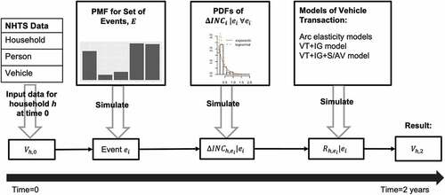
The amount of income change that occurs for the first four events, $\left(\mathrm{\Delta }IN{C}_{h,e_i}|e_i\right),i=1,2,3,4$, is predicted (Section 4.3). The resulting distribution of the simulated income changes following events 1–4 in the NHTS data is shown in Figure 5. With the income changes, we simulate the vehicle transaction response ($R_{h,e_i}|e_i$) of the household to the stimulating event. We use $V_{h,2}$ to denote the predicted, short-term HHVO of household $h$ after responding to the simulated income change event.

Figure 5. Frequency distribution of simulated income changes.

The alternative models for estimating vehicle transaction use arc elasticities of vehicle transaction with respect to household income. Arc elasticities are estimated using the Puget Sound data and are specific to each type of the above income changing events. Each model is applied by multiplying the event-specific arc elasticity with the simulated income change.

With the simulated income change events, three vehicle transaction simulations are performed

• Simulation 1: Vehicle ownership without sharing economy.

• Simulation 2: Vehicle ownership in a sharing economy.

• Simulation 3: Vehicle ownership in a sharing economy with AV options.

The three simulations rely on different means for estimating vehicle transactions, as shown in Table 5. For event 4, since the new job is within one mile of home and/or accessible by transit, which is different from our choice experiment context, neither the VT+IG nor VG+IG+S/AV model should be used. Therefore, arc elasticities are used.

Table 5. Summary of vehicle ownership models and their use during the simulation

Household income event	Vehicle ownership model used in:
	Simulation 1	Simulation 2	Simulation 3
Event 1	Arc elasticity for Event 1	VT+IG model	VT+IG+S/AV model
Event 2	Arc elasticity for Event 2	VT+IG model	VT+IG+S/AV model
Event 3	Arc elasticity for Event 3	VT+IG model	VT+IG+S/AV model
Event 4	Arc elasticity for Event 4	Arc elasticity for Event 4	Arc elasticity for Event 4
Event 5	Arc elasticity for Event 5	Arc elasticity for Event 5	Arc elasticity for Event 5

Analysis of Puget sound data to develop additional simulation models

As mentioned before, survey data for the Puget Sound region in the state of Washington, collected by the Puget Sound Council of Governments (now the Puget Sound Regional Council) (Murakami and Watterson 1990), are used to develop three models for the simulation:

1. A probabilistic model of (discrete) household income change events;

2. A probabilistic model of the (continuous) change in household income that occurs when a household experiences an income change event;

3. A model that predicts vehicle transaction decisions by households in response to changes in household income absent the sharing economy and vehicle automation.

The rest of Section 4.3 describes the Puget Sound data and how the data are used to develop these three models for the simulation. Next, Section 4.4 describes the application of each of the three models. Figure 4 and Table 5 serve to guide the reader in understanding each model and its place in the simulation setup.

The Puget Sound data provide information on household income changes, HHVO changes, job changes, and other changes, in 1989, 1990, 1992, 1993, 1994, 1996, 1997, 1999, 2000 and 2002. The analysis here focuses on changes between data collection years (1989–1990, 1990–1992, etc.). The associated data contain about 7,700 households. For simplicity, the current analysis ignores potential autocorrelation as well as life-cycle effects, such as retiring, under the assumption that households do not move residences in the short-term. These factors may be addressed in follow-up work.

The probabilistic model of household income change events predicts the probability that each event type occurs in the short term. For a household, exactly one event is simulated. This process is necessary because households experience various vehicle transaction-triggering events at different times and frequencies. The simulation is based on a probability mass function (pmf) of job and income change events relevant to this analysis, which is constructed using the Puget Sound data as shown in Figure 6.

Figure 6. Probability mass function of simulated income change events.

Events that ‘match’ the two SP contexts in our survey are simulated along with events that are not consistent with the SP contexts, such as the event of a new job that is accessible by transit. The matching events from the Puget Sound data are identified based on the following criteria. A decrease in household income between two consecutive panels is treated as a ‘match’ to the income decrease context in our SP survey. An increase in household income between two consecutive panels that is accompanied by (1) a change in workplace location and (2) the new workplace being greater than one mile from home and not located in downtown Seattle is treated as a ‘match’ to the income increase context in our SP survey. The workplace location criteria are based on the fact that downtown Seattle has good transit accessibility and the observation that personal auto dominates work mode share in other cases. The pmf also includes an event that involves an increase in income that does not meet these criteria. Finally, the ‘No change/Other’ category covers households that have no income changes.

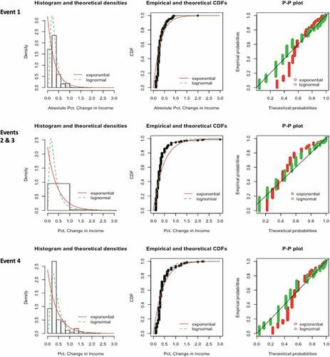
In the event of income change, the amount of income increase or decrease then is simulated based on observed distributions from the Puget Sound data. The Puget Sound data are used to develop probabilistic models of absolute change in income that is associated with each event (Figure 7) (plots are generated using Delignette-Muller and Dutang 2020). Lognormal and exponential distributions are explored for events that correspond to the SP scenarios. Akaike’s Information Criterion (AIC) is used to compare the relative strength of fit for the two distributions. The AIC for the lognormal (exponential) fit is −256.5 (348.2). Lower AIC indicates a better fit, therefore lognormal is a better fit than exponential for this distribution. Consequently, lognormal distributions are adopted, and Monte Carlo draws are used to simulate income changes for all events that have an income change. Since the draw generates an absolute change in percentage, the drawn number is converted to a negative in the case of an income loss event.

Figure 7. Income change distributions for household income events.

Finally, the model that predicts vehicle transaction decisions is developed based on arc elasticities with respect to household income derived from the Puget Sound data, as shown in Table 6. These elasticities are in line with the literature (e.g., Goodwin, Dargay, and Hanly 2003; Litman 2019). We note that the elasticity with respect to income decrease is quite low (0.012) in times of economic upturn (1993–2000), and much greater (0.27) in times of economic downturn. One possible explanation is that in times of significant macroeconomic declines, households are more likely to shed vehicles, while in times of broad economic health households have more optimism and tend to maintain their fleets. Assuming that the economy will be in a major downturn in three out of the next ten years, the elasticity associated with a major economic downturn is applied randomly to 30% of the households that will suffer an income decrease. For the remaining households with an income decrease, the upturn rate of 0.012 is applied.

Table 6. Arc elasticities derived from Puget sound data.

Population-level elasticities of HHVO with respect to household income
Households with income increase & SP Context 1 (≥15 mi)	0.23
Households with income increase & SP Context 2 (1–15 mi)	0.15
Households with income increase, Non-SP Context	0.46
Households with income decrease - major downturn (based on 2000–2002 data) - economic upturn (based on 1993–2000 data)	0.27 0.012

For events that do not match one of the SP contexts, a net of 1.7% of households undergo a gain of one vehicle and 0.7% had a gain of two. Other gains and losses are observed but not worth modeling since these details would effectively cancel each other out when the results are aggregated across the population.

Simulations 1 and 2: without and with sharing economy

In a simulation, each household experiences one of the five income change events. Household events are simulated using Monte Carlo draws and the observed probabilities as shown in Figure 6. The arc elasticities and the other rates (1.7% (0.7%) for a gain of 1 (2) vehicles) are applied to predict response to the event for Simulation 1 (base case), while the VT+IG model is applied in Simulation 2 to replace the base case results for households with events that match an SP Context. The results are shown in Table 7. HHVO indicates the number of vehicles in a household in the base year. For a given HHVO category, HH under ‘Base Year’ indicates the number of households in the NHTS data that have the number of vehicles as HHVO. HHV under ‘Base Year’ is the total number of household vehicles in the corresponding category, equal to HHVO times HH (though the displayed numbers are not exact due to rounding errors).

Table 7. Results from simulations 1 and 2.

Category	Base Year		Simulation 1 (w/o sharing economy)		Simulation 2 (w/ sharing economy)
HHVO	HH^*,1	HHV^*,2	HHV	Avg. number of new vehicles per HH	HHV	Avg. number of new vehicles per HH
0	10,567	0	565	0.05	1,281	0.12
1	39,648	39,648	41,803	1.05	44,298	1.12
2	39,125	78,250	80,429	2.06	82,565	2.11
3	17,598	52,794	53,754	3.05	54,727	3.11
4	7,194	28,776	29,163	4.05	29,574	4.11
5	2,579	12,896	13,030	5.05	13,182	5.11
6	848	5,089	5,132	6.05	5,159	6.08
7	378	2,646	2,664	7.05	2,683	7.10
8	130	1,040	1,047	8.05	1,056	8.13
9	62	554	558	9.07	558	9.05
10	26	262	264	10.07	264	10.08
11	21	230	232	11.10	232	11.12
12	33	393	394	12.03	397	12.12
Total	118,208	222,579	229,036		235,977
% increase over Base Year:			2.9%		6.0%

* All counts of households and vehicle population are in 1,000s.

¹HH is the number of households corresponding to each Base Year HHVO level.

²HHV is the total number of vehicles owned by households from each Base Year HHVO category.

For simulation 1 (without sharing economy), we find the total number of household vehicles would increase from 222,579 to 229,036, or a 2.9% increase. This rate is comparable to the 2.8% historical average annual increase (1950–2016) (Oak Ridge National Laboratory 2019). For simulation 2, which considers a sharing economy and uses the VT+IG model, a 6% growth in household vehicle ownership is found, which provides strong evidence that the population of household vehicles will increase more when the vehicles can be used for income earning under sharing economy. It should be noted that the projected growth is based on SP data, and therefore should be interpreted conservatively. Furthermore, the share of households that use a vehicle to earn income is predicted to grow from 5.1% of households to about 7–8% as the adoption of the sharing economy paradigm continues in the transportation system. While this percentage does not consider attrition, which is high for certain types of labor (McGee 2017), the percentage nevertheless suggests that many individuals will continue to consider the income generation potential of vehicles when experiencing events that lead to vehicle transaction decisions.

Simulation 3: with sharing economy and vehicle automatio

Table 8 reports vehicle ownership results from Simulation 3, which is with sharing economy and AVs. The results are also compared with the Base Year. Two differences from Table 7 are worth noting. First, the scenario results are delineated by the Analysis of Owned Vehicles, which includes both CVs and AVs, and the Analysis of Vehicle Sharing that focuses on predicted SAV use. Second, total new household vehicles (HHV (before reduction)) is the sum of CVs and AVs that are predicted to be purchased. Recalling that choice experiment 4 asks respondents who currently own one or more CVs and choose AV/SAV options about CV disposal, the ownership estimate is further refined to account for the CV disposal effect. The disposal rate comes directly from choice experiment 4. On average, individuals who choose AV or SAV in the survey indicate that their households would dispose of 0.3 vehicles from the existing fleet. The disposal rate is applied to the household of each individual that is predicted to choose AV or SAV, to compute a reduction in the number of household vehicles owned (HHV reduction).

Table 8. Results from simulation 3.

Cate-gory	Base Year		Simulation 3 (w/ sharing economy and vehicle automation)
HHVO	HH^*,1	HHV^2	Analysis of Owned Vehicles			Analysis of Vehicle Sharing		HHV after reduction
			HHV (before reduction)		HHV reduction	HH: join SAV	HHV reduction
			CV + AV	AV Only
0	10,567	0	1,008	154		98	-	1,008
1	39,648	39,648	43,913	571	−171	252	−75	43,666
2	39,125	78,250	82,686	607	−182	347	−104	82,399
3	17,598	52,794	54,829	300	−90	163	−49	54,690
4	7,194	28,776	29,609	128	−38	66	−20	29,550
5	2,579	12,896	13,193	48	−14	25	−7.5	13,171
6	848	5,089	5,175	11	−3.3	7.4	−2.2	5,169
7	378	2,646	2,686	9	−2.6	2.2	−0.66	2,682
8	130	1,040	1,058	2	−.6	0.93	−0.28	1,057
9	62	554	560			-	-	560
10	26	262	266			-	-	266
11	21	230	233			-	-	233
12	33	393	396	1	−.3	-	-	396
Total	118,208	222,579	235,611	1,831	−503	962	−259	234,849
% increase over Base Year:			5.9%					5.5%

* All counts of household and vehicle population are in 1,000s.

¹HH is the number of households corresponding to each Base Year HHVO level.

²HHV is the total number of vehicles owned by households from each Base Year HHVO category.

As is shown at the bottom of Table 8, before accounting for HHV reduction, it is estimated that total vehicle population would increase by 5.9%, which is similar to the result under the sharing economy scenario. Based on this simulation analysis, it is reasonable to attribute this increase to a combination of sharing economy impacts and people’s interest in AV adoption. On the other hand, when vehicle disposal with AV/SAV is considered, the total vehicle population is predicted to increase by 5.5% instead of 5.9%, which is in line with previous findings of reduced aggregate HHVO due to AV/SAV use (Fagnant and Kockelman 2014; Auld et al. 2018).

As a final note, since the main goal of this paper is to understand the directionality and approximate magnitude of the sharing economy and vehicle automation impacts, calibration and validation are not considered essential at this point. Undertaking calibration and validation are expected, in this case, to lead to the same general conclusions that the sharing economy and vehicle automation would increase HHVO compared to a world without them. Nevertheless, it is worth mentioning that the magnitude of the simulation estimations should be interpreted with this caveat in mind.

Conclusions

This study hypothesizes that the sharing economy has led many individuals to consider the potential of earning income using household vehicles when making household vehicle ownership decisions. To this end, using data collected from an original survey, two discrete choice models are developed to reveal the various factors that influence vehicle ownership decisions. These models investigate vehicle investment decisions from different perspectives. The first is the propensity for vehicle transaction resulting from changes in income. The second is vehicle ownership choice in the advent of autonomous vehicles and shared autonomous mobility services.

The estimation results yield several interesting insights. Foremost, income earning potential is confirmed to stimulate vehicle ownership. If household income were decreased, some individuals would prefer to keep their fleets and use a vehicle to earn income rather than to sell a vehicle. If household income were increased, the potential for extra income generation would inspire some individuals to purchase a vehicle. Income generation potential of household-owned AV likewise influences individuals to own an AV over owning a CV or using SAV.

The estimated models are also used to assess the impact of the sharing economy and vehicle automation on short-term vehicle ownership at the national level. We find that in the sharing economy, household vehicle ownership levels are higher than they otherwise would be without such options available. Further, the sharing economy along with the options of owning or sharing AVs would lead to higher vehicle ownership levels than a future without these options. The findings suggest that additional economic and policy interventions would be needed if reduced vehicle ownership is the desired outcome in the presence of the sharing economy and vehicle automation.

While an increasing consensus is emerging that human mobility is heading toward a shared, autonomous future, almost no attention has been paid so far to the implications for vehicle ownership due to the new opportunities for using owned vehicles to generate extra income for households. This research shows a promising beginning toward understanding this overlooked issue. Future work can be extended in a few directions. First, the models developed in this paper can be further refined with the collection and incorporation of land use information, which influences vehicle ownership decisions and may someday be affected by the expansion of autonomous vehicle use. Second, as ridesourcing has become commonplace in society and mobility services provided by shared autonomous vehicles are rapidly developing, conducting revealed preference (RP) surveys and combining SP with RP data for further model development could lead to improved estimates of the model coefficients. Third, a longitudinal survey that follows a panel of households over the next several years would provide rich data to improve these models and other models that predict the impacts of technological innovations on vehicle ownership and the transportation system. Finally, data from the earnings preference questions in the survey currently are being explored by us to jointly examine earning potential and vehicle transactions. The results may yield further insights about vehicle ownership with sharing economy and vehicle automation effects.

Acknowledgments

The authors are grateful to the Puget Sound Regional Council (formerly the Puget Sound Council of Governments) for providing the panel data used in this study. The authors are grateful to Samar Ahmed for assistance with data collection and data quality control. The submission has been created in part by Uchicago Argonne, LLC, Operator of Argonne National Laboratory (“Argonne”). Argonne, a U.S. Department of Energy Office of Science laboratory, is funded and operated under Contract No. DE-AC02-06CH11357. The U.S. Government retains for itself, and others acting on its behalf, a paid-up, nonexclusive, irrevocable worldwide license in said article to reproduce, prepare derivative works, distribute copies to the public, and perform publicly and display publicly, by or on behalf of the Government. Bo Zou was also supported in part by the National Science Foundation under grant CMMI-1663411.

Disclosure statement

No potential conflict of interest was reported by the author(s).

Additional information

Funding

This work was supported by the Argonne National Laboratory [DE-AC02-06CH11357]; National Science Foundation [CMMI-1663411].

Notes

1. Sample size was not determined a priori, since with the innovative nature of this study the model specification was not known beforehand. However, the study team aimed to collect at least 500 surveys in total based on collective experience of the study team members.

Appendix A:

Survey instrument

Appendix B:

Additional descriptive statistics

This appendix presents some additional descriptive statistics of the data. First, pair plots of the frequency of using different modes, including driving, riding, ridesourcing, transit, and nonmotorized modes, are shown in Figure A1. Taxi and carshare are not presented as they are used much less frequently than those modes. In A1, a function is applied to each point to slightly shift it away from the actual point so that a pseudo-density can be envisioned (Wilke 2019). Abbreviations in the figure are: fdrv = frequency of driving, fride = frequency of getting a ride (from a family member or a friend), frsource = frequency of ridesourcing (such as Lyft or Uber), fxit = frequency of transit, and fnonmot = frequency of nonmotorized modes. The responses are categorical, with 4 = more than once a week, 3 = about once a week, 2 = once a month or less, and 1 = never.

Figure A1 shows a broad and balanced range of travel habits among surveyed individuals. Some interesting observations can be gained. For example, individuals who drive more than once a week (category 4) tend to get a ride or take ridesourcing less frequently, only once per month or never. Low frequency of getting a ride is typically associated with rare use of ridesourcing. For driving, high frequency does not clearly connect with the frequency of taking transit or nonmotorized modes. But the usage frequencies of transit and nonmotorized modes are strongly correlated.

Figure A1. Frequency of using various modes.

Figure A2 shows the frequency distributions of some sociodemographic characteristics. The sample is almost evenly split between females and males (Figure A2-A). Most respondents have an Associate degree or higher education level (Figure A2-B). Further analysis shows that the remaining 10% is evenly split between current college students and those who are not enrolled in college. A broad range of household sizes is captured (Figure A2-C). Most respondents come from households with multiple workers (Figure A2-D). Households both with and without children are well represented (Figure A2-E). The survey also has a good representation of students and non-students (Figure A2-F). About 10% of the respondents come from households with one or more vehicles used for income generation purposes (Figure A2-G). The charted percentage of respondents by income level (Figure A2-H) shows that about half of the respondents earn more than $75,000. Finally, the age distribution is skewed toward younger people (Figure A2-I). The age distribution is in line with the share of student respondents.

Figure A2. Sociodemographic characteristics of sample.

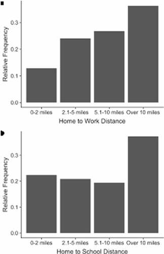
Figure A3 shows the commute distances to work and school among respondents in the sample. The reported home-to-work distance (Figure A3-A) appears farther than the home-to-school distance (Figure A3-B).

Figure A3. Commute distance characteristics of sample.

Appendix C:

Model sensitivity

This appendix presents and discusses the sensitivity of the VT+IG model to variations in a key explanatory variable (change in income). The differences in response to income change in the VT+IG+S/AV model by household income segment is also presented.

Figure A4 shows the sensitivity of the VT+IG model prediction to income change. As seen in this figure and noted in Section 3, based on the model results, individuals are much more likely to make some change in fleet or vehicle use (in comparison with None) when the income change is positive than when the income change is negative. In income loss scenarios, however, most persons will choose None, suggesting that individuals may optimistically believe that their households will soon recover the lost income level and therefore see no need to change their fleets or work habits. It is important to remember that in the case of a positive income change, the context of the SP question centered around a new job that could not be reached by transit. Therefore, it is expected that the VT+IG model coefficients will generate relatively high rates of vehicle purchases (as discussed in Section 3) for individuals in this circumstance.

Figure A4. Sensitivity of VT+IG choice to change in income.

These outcomes provide behavioral evidence that the sharing economy impacts vehicle transaction decisions. Two phenomena are especially worth mentioning. First, the potential to earn income incentivizes individuals to purchase a vehicle. Based on the model prediction, a relatively large number of individuals (about 20% to 25%) would both purchase a new vehicle and use it to earn income. This is quite notable considering that in the context of the SP questions individuals would already be enjoying higher incomes due to a new job. Second, the potential to earn income makes it easier for individuals to keep the existing fleet even in times of income loss – this figure shows that in times of income loss, the behavioral response involves a reluctance to part with vehicles. Individuals expressed a greater preference to earn income with a vehicle rather than sell it in these situations. Together, these behavioral effects imply that vehicle ownership levels in the sharing economy will either stay the same or increase, all else equal, in comparison with vehicle ownership levels in a non-sharing economy.

Figure A5 portrays the predicted market shares by the VT+IG+S/AV model for various household income levels. The estimates are based on an annual household income increase of $5,000. As with the VT+IG model, the SP context involved a distant new job with an income increase; therefore, the share of individuals that either buy a new vehicle or join an AV-share program as expected is relatively high. The preference of ‘None’ (no change in fleet) is greatest for low-income household and diminishes with increasing income. This may reflect the preference of low-income households to spend the new extra income on other things besides transportation. Also, as income increases, the interest in AV-share options increases. This may reflect the willingness of wealthier individuals to experiment with new modes.

Figure A5. Variation in vehicle transaction choice by household income level in a futuristic context.

References

- Alonso-González, M. J., O. Cats, N. van Oort, S. Hoogendoorn-Lanser, and S. Hoogendoorn. 2020. “What are the Determinants of the Willingness to Share Rides in Pooled On-demand Services?” Transportation. doi:10.1007/s11116-020-10110-2.
- Auld, J., O. Verbas, M. Javanmardi, and A. Rousseau. 2018. “Impact of Privately-Owned Level 4 CAV Technologies on Travel Demand and Energy.” Procedia Computer Science 130: 914–919. doi:10.1016/j.procs.2018.04.089.
- Ben-Akiva, M., and S. Lerman. 1985. Discrete Choice Analysis. Cambridge, MA: MIT Press.
- Bierlaire, M., 2014. “Discrete Panel Data. Transport and Mobility Laboratory, School of Architecture, Civil and Environmental Engineering.” Ecole Polytechnique Federale de Lausanne. Accessed on 1 March 2021. https://transp-or.epfl.ch/courses/dca2014/slides/12-panel.pdf
- Bierlaire, M., 2016. “To Be or Not to Be Significant.” Video recording, Accessed on 1 March 2021. https://biogeme.epfl.ch/videos.html#toBe
- Bierlaire, M., 2018. “PandasBiogeme: A Short Introduction. Technical Report TRANSP-OR 181219.” Transport and Mobility Laboratory, ENAC, EPFL.
- Bischoff, J., and M. Maciejewski. 2016. “Autonomous Taxicabs in Berlin–a Spatiotemporal Analysis of Service Performance.” Transportation Research Procedia 19: 176–186. doi:10.1016/j.trpro.2016.12.078.
- Boesch, P. M., F. Ciari, and K. W. Axhausen. 2016. “Autonomous Vehicle Fleet Sizes Required to Serve Different Levels of Demand.” Transportation Research Record: Journal of the Transportation Research Board 2542 (1): 111–119. doi:10.3141/2542-13.
- Botsman, R., and R. Rogers. 2010. What’s Mine Is Yours: The Rise of Collaborative Consumption. New York: Harper Business.
- Bustamante, J., 2019. “College Enrollment Statistics & Student Demographic Statistics.” [WWW Document]. EDUCATIONDATA.ORG, (Accessed 1 February 2020). https://educationdata.org/college-enrollment-statistics/
- Campbell, H. 2018. “Who Will Own and Have Propriety over Our Automated Future? considering Governance of Ownership to Maximize Access.” Efficiency, and Equity in Cities,” Transportation Research Record 2672 (7): 14–23. doi:10.1177/0361198118796392.
- Cervero, R., A. Golub, and B. Nee. 2007. “City CarShare: Longer-Term Travel Demand and Car Ownership Impacts.” Transportation Research Record: Journal of the Transportation Research Board 1992 (1): 70–80. doi:10.3141/1992-09.
- Chen, T. D., K. M. Kockelman, and J. P. Hanna. 2016. “Operations of a Shared, Autonomous, Electric Vehicle Fleet: Implications of Vehicle & Charging Infrastructure Decisions.” Transportation Research Part A: Policy and Practice 94: 243–254.
- Chicago Transit Authority, 2021. “Unlimited Ride Passes. [WWW Document].” (Accessed 4 November 2021). https://www.transitchicago.com/passes
- Costain, C., C. Ardron, and K. N. Habib. 2012. “Synopsis of Users’ Behaviour of A Carsharing Program: A Case Study in Toronto.” Transportation Research Part A: Policy and Practice 46: 421–434.
- Delignette-Muller, M., and C. Dutang, 2020. “Fitdistrplus: An R Package for Fitting Distributions Dutang.” Universite de Lyon and Universite de Strasbourg. Accessed on 1 March 2021. https://cran.r-project.org/web/packages/fitdistrplus/vignettes/paper2JSS.pdf
- Deloitte, 2016. “The Future of Mobility – What’s Next? [WWW Document].” (accessed 20 July 2019). https://www2.deloitte.com/za/en/pages/consumer-industrial-products/articles/the_future_of_mobility_whats_next.html
- Edmunds, 2020. “Average down Payments for New Vehicles See a Big Lift in Q3, according to Edmunds.” [WWW Document], (Accessed 11 April 2021). https://www.edmunds.com/industry/press/average-down-payments-for-new-vehicles-see-a-big-lift-in-q3-according-to-edmunds.html
- Experian, 2017. “The Average Amount Financed for New and Used Vehicles Hit Record Highs, Making Longer-term Loans More Popular among Consumers.” [WWW Document], (Accessed 11 April 2021). https://www.experianplc.com/media/news/2017/q4-state-of-the-automotive-finance-market-report
- Fagnant, D. J., and K. M. Kockelman. 2014. “The Travel and Environmental Implications of Shared Autonomous Vehicles, Using Agent-based Model Scenarios.” Transportation Research Part C: Emerging Technologies 40: 1–13. doi:10.1016/j.trc.2013.12.001.
- Federal Highway Administration, 2017. “National Household Travel Survey [WWW Document].” https://nhts.ornl.gov
- Goodwin, P., J. Dargay, and M. Hanly. 2003. “Elasticities of Road Traffic and Fuel Consumption with respect to Price and Income: A Review.” Transport Reviews 24 (3): 275–292. doi:10.1080/0144164042000181725.
- Gurumurthy, K. M., K. M. Kockelman, and M. D. Simoni. 2019. “Benefits and Costs of Ride-Sharing in Shared Automated Vehicles across Austin, Texas: Opportunities for Congestion Pricing.” Transportation Research Record 2673 (6): 548–556. doi:10.1177/0361198119850785.
- Heilig, M., T. Hilgert, N. Mallig, M. Kagerbauer, and P. Vortisch. 2017. “Potentials of Autonomous Vehicles in a Changing Private Transportation System–a Case Study in the Stuttgart Region.” Transportation Research Procedia 26: 13–21. doi:10.1016/j.trpro.2017.07.004.
- Hughes, C., 2018. “Uber Wants to Ban Private Autonomous Vehicles [WWW Document].” Economics21: Manhattan Institute for Policy Research. (Accessed 20 July 2019). https://economics21.org/html/uber-wants-ban-private-autonomous-vehicles-2834.html
- Javanmardi, M., J. Auld, and K. Gurumurthy. 2019. “Intra-Household Fully Automated Vehicles Assignment Problem: Model Development and Case Study.”
- Jin, S. T., H. Kong, R. Wu, and D. Z. Sui. 2018. “Ridesourcing, the Sharing Economy, and the Future of Cities.” Cities 76: 96–104. doi:10.1016/j.cities.2018.01.012.
- Litman, T. 2019. Understanding Transport Demands and Elasticities: How Prices and Other Factors Affect Travel Behavior. Victoria, British Columbia: Victoria Transport Policy Institute.
- Louviere, J., D. Hensher, J. Swait, and W. Adamowicz. 2000. Stated Choice Methods: Analysis and Applications. Cambridge: Cambridge University Press.
- Manski, C., and D. McFadden. 1981. Alternative Estimators and Sample Designs for Discrete Choice Analysis, In: Structural Analysis of Discrete Data with Econometric Applications. Cambridge, Massachusetts: MIT Press.
- Martin, E., S. A. Shaheen, and J. Lidicker. 2010. “Impact of Carsharing on Household Vehicle Holdings: Results from North American Shared-Use Vehicle Survey.” Transportation Research Record: Journal of the Transportation Research Board 2143 (1): 150–158. doi:10.3141/2143-19.
- Martinez, L. M., and J. M. Viegas. 2017. “Assessing the Impacts of Deploying a Shared Self-driving Urban Mobility System: An Agent-based Model Applied to the City of Lisbon, Portugal.” International Journal of Transportation Science and Technology 6 (1): 13–27. doi:10.1016/j.ijtst.2017.05.005.
- McGee, C., 2017. “Only 4% of Uber Drivers Remain on the Platform a Year Later, Says Report [WWW Document].” CNBC, (Accessed 21 July 2019). https://www.cnbc.com/2017/04/20/only-4-percent-of-uber-drivers-remain-after-a-year-says-report.html
- Metra, 2021. “Ticket Options.” [WWW Document], (Accessed 11 April 2021). https://metrarail.com/tickets
- Mitchell, R. 2019. “In a Bind, Musk Hopes Autonomous Tesla Taxis Will Drive a New, Positive Narrative [WWW Document].” Los Angeles Times, (Accessed 20 July 2019). https://www.latimes.com/business/autos/la-fi-hy-tesla-elon-musk-full-self-drive-model3-demand-cash-20190419-story.html
- Murakami, E., and W. T. Watterson. 1990. “Developing a Household Travel Panel Survey for the Puget Sound Region.“ Transportation Research Record 1285: 40–46.
- Noruzoliaee, M., and B. Zou. 2022. “One-to-many Matching and Section-based Formulation of Autonomous Ridesharing Equilibrium.“ Transportation Research Part B: Methodological 155: 72–100. doi:10.1016/j.trb.2021.11.002.
- Noruzoliaee, M., B. Zou, and Y. Liu. 2018. “Roads in Transition: Integrated Modeling of a Manufacturer-traveler-infrastructure System in a Mixed Autonomous/human Driving Environment.” Transportation Research Part C: Emerging Technologies 90: 307–333. doi:10.1016/j.trc.2018.03.014.
- Oak Ridge National Laboratory. 2019. “Household Vehicles and Characteristics - Transportation Energy Data Book: Edition 37, Chapter 8 [WWW Document].” (Accessed 19 April 2019). https://cta.ornl.gov/data/chapter8.shtml
- Schaller, B., 2017. “UNSUSTAINABLE?” The Growth of App-Based Ride Services and Traffic, Travel and the Future of New York City [WWW Document], Accessed 9 February 2019. http://schallerconsult.com/rideservices/unsustainable.htm
- Simoni, M. D., K. M. Kockelman, K. M. Gurumurthy, and J. Bischoff. 2019. “Congestion Pricing in a World of Self-driving Vehicles: An Analysis of Different Strategies in Alternative Future Scenarios. Transportation Research Part C.” Transportation Research Part C: Emerging Technologies 98: 167–185. doi:10.1016/j.trc.2018.11.002.
- Spieser, K., S. Samaranayake, W. Gruel, and E. Frazzoli. 2016. Shared-vehicle Mobility-on-demand Systems: A Fleet Operator’s Guide to Rebalancing Empty Vehicles. Washington DC: Transportation Research Board 95th Annual Meeting.
- US Census, 2011. “Age and Sex Composition: 2010, 2010 Census Briefs.” Accessed 20 January 2020. https://www.census.gov/prod/cen2010/briefs/c2010br-03.pdf
- Wilke, C., 2019. “Cowplot: Streamlined Plot Theme and Plot Annotations for ‘Ggplot2ʹ.” (Accessed 1 February 2020). https://www.r-pkg.org/pkg/cowplot