Research on the combinatorial optimization of EBs departure interval and vehicle configuration based on uncertain bi-level programming

ABSTRACT

Based on uncertainty theory, this paper proposed a vehicle scheduling method considering the dynamic departure interval and vehicle configuration of electric buses (EBs). An uncertain bi-level programming model (UBPM) is established, which takes the total cost of passenger travel (CP) as the upper and total cost of EBs (CB) as the lower. A chance constrained programming model (CCPM) based on the randomness of passenger waiting time and the uncertainty of interstation running time is proposed as the upper model. With a certain confidence level of service level as constraints, the goal is to minimize the total cost of passenger travel. Then, an expected value model (EVM) based on the fluctuation of energy consumption is proposed as the lower model. Taking the number of EBs as the constraint condition, the goal was to minimize the energy consumption of EBs. Finally, a practical bus route is taken as an example to verify the effectiveness of the proposed method. The results demonstrated that the optimal scheduling plan considering the uncertain variables can reduce the passenger travel cost. Collaborative optimization of EBs vehicle configuration can reduce energy consumption, delay, and the number of EBs.

KEYWORDS:

• Electric buses
• uncertainty theory
• bi-level programming
• timetable optimization
• vehicle configuration

Introduction

Compared with other modes of transport, public transport has the advantages of efficiency, energy conservation, and environment protection. Meanwhile, it can alleviate traffic congestion and provide convenience for passengers. Public transportation optimization is conducive to the sustainable operation of the bus system, including four parts: Transit Network Design, Transit Network Timetabling problem, Operational planning decisions, and Real-time control strategies, among which the latter part depends on the former part. For example, different frequencies may imply different vehicle schedules and passenger wait time which strongly influence operational costs and passenger cost. Therefore, a complete consideration of all the subproblems of transit network planning is feasible. However, the four sub-problems of public transportation system are all complicated and affected by uncertain factors in the process of operation. In the design of the transportation network, routes and stations are laid out using preconceived transportation network timetables. After the completion of the design of the transportation network, the frequency and timetables of departures should be set according to the routes and stops. Setting the completed timetables affects not only the next operational planning decisions but also the original line and stops, thus creating a cycle. Among them, transportation network timetables not only play a key role in the efficient operation of subsequent traffic, but also have a direct impact on the attractiveness of passengers. However, due to the diversity of passenger demand and the complexity of traffic conditions, the timetables can only meet the requirements of most passengers in a specific period of time, which is inconsistent with the dynamic passenger flow demand in reality.

Due to various uncertainties in the reality (e.g. passenger demand, etc.), bus timetables optimization does not accord with the reality, thus affecting the entire bus system, resulting in resource waste and inefficiency. A solution is to design a bus scheme that considers uncertain factors (e.g. passenger demand (Zhan et al. 2017; Zhang, Wang, and Meng 2020), climate change (Amiripour, Ceder, and Mohaymany 2014; Uchida, Sumalee, and Ho 2015), etc.). When optimizing the line network (Li et al. 2021; Ghaffari, Mesbah, and Khodaii 2020), timetabling (Gkiotsalitis 2021; Gkiotsalitis and Alesiani 2019; David and Kresz 2020; Xu et al. 2009) and vehicle scheduling (Shen, Xu, and Li 2016; Yan and Tang 2008, 2009; Liu and He 2006; Wei 2012), scholars have considered uncertain factors such as travel time (Bie et al. 2021; Huang, Ren, and Liu 2013; Yan, Hsiao, and Chen 2015; Zhang and Tang 2014), passenger demand (Kulshrestha, Lou, and Yin 2014; Li, Lam, and Wong 2011; Sun et al. 2018), seasonal variation (Amiripour, Ceder, and Mohaymany 2014), and random environment (Zhang and Guang 2014), e.g. Wei (2012) optimized regional vehicle scheduling based on the uncertainty of travel time, Sun et al. (2018) optimized the transfer bus scheduling based on the theory of cluster analysis, Konstantinos (2019) optimized the bus schedule based on the uncertainty of travel time and passenger demand. However, in the process of modeling, it is assumed that passenger demand follows normal distribution or uniform distribution, which is different from the uncertain distribution of passenger arrival demand in reality. Moreover, only single vehicle model and single uncertainty factors are considered, which is inconsistent with the actual operation of public transport. In this paper, the discrete distribution of passenger arrival follows the Poisson distribution, and passengers are independent of each other. The waiting process is considered as a Markov process. In addition, on the basis of considering passenger demand, two uncertainties including interstation running time and EBs energy consumption are also considered.

Timetabling and vehicle scheduling, as the transitional section of the bus system, have been concerned by scholars. For the vehicle models mentioned in the above paragraph, some scholars have considered the combination of multiple models (Ding 2017; Wang 2018) and even combined with the bus schedule (Huang et al. 2016; Yao et al. 2020). For example, Yao et al. (2020) proposed the method of optimizing the departure interval and vehicle-type configuration of conventional bus lines in the mixed-model operation, and Huang et al. (2016) studied the departure frequency of the multi-model bus system. However, due to the complexity of the actual situation, it is assumed that the passenger arrival rate is uniform and does not consider the existing uncertain factors. The established vehicle scheduling model has been studied by some scholars and is usually solved by genetic algorithm (Baita et al. 2000; Huang, Ren, and Liu 2013), heuristic algorithm (Yao et al. 2016), and intelligent algorithm (Xu et al. 2009). Recent studies can also be referred to Zhang, Zhao, and Xu (2021) and Zhang, Zeng, and Gao (2022). However, genetic algorithm and heuristic algorithm cannot guarantee the global optimal solution. The precise intelligent algorithm is time-consuming and has a large amount of data, which requires high bus cost.

Although optimization of bus scheduling can improve the efficiency of bus operation and passenger satisfaction, the cost of optimization is limited. To maximize the income of public transportation and meet the needs of passengers, relevant scholars usually adopt the bi-level programming model (BPM) (Ci, Han, and Wu 2021; Liu and Shen 2007; Yan and Guang 2008). Yan and Tang (2008), Ci, Han, and Wu (2021) established a BPM with passenger satisfaction as the upper and enterprise operation efficiency as the lower, while Liu and Shen (2007) established a BPM with opposite upper and lower targets. In addition, uncertain factors were considered in the BPM established by Wei, Sun, and Jin (2013), and Xue et al. (2020). The balance between bus cost and efficiency is well solved by the BPM, but the fluctuation of energy consumption is not considered. With the popularization of EBs, the study considering the volatility of energy consumption deserves further discussion. In the context that China ranks first in the production, sales, and usage of new energy automobiles in the world, reducing energy consumption of EBs will promote the construction of transit metropolis and fulfill the ‘Carbon Peak and Carbon Neutrality’ goals.

Based on the above research, this paper proposes a vehicle scheduling method with a dynamic departure interval and EBs combination considering multiple uncertainties. An uncertain bi-level programming model (UBPM) is established, which takes the total passenger travel cost as the upper and the energy consumption of EBs as the lower. The model considers a variety of vehicle types, passenger demands, and energy consumption. A genetic algorithm with an elite retention strategy is adopted to solve the problem, which reduces the complexity and improves the efficiency. Different from previous studies:

(1) When solving the calculation of passenger waiting time, the discrete distribution of passenger arrival and the continuous distribution of waiting time of each passenger arrival are considered as a composite Poisson process, which satisfies the Markov process.

(2) By establishing UBPM, this paper considers four uncertain variables: the number of passenger arrival, the waiting time of passengers, the interstation running time, and the energy consumption of EBs. The distribution functions of four uncertain variables are given for quantitative analysis. Based on UBPM, the scheduling scheme of dynamic bus departure interval and vehicle type combination in different time periods is presented.

(3) Not only the uncertain variables are considered, but also the EBs model configuration is considered. The uncertainty theory adopted is a synthesis of three major theories (probability theory, reliability theory, and credibility theory) and has wider applicability.

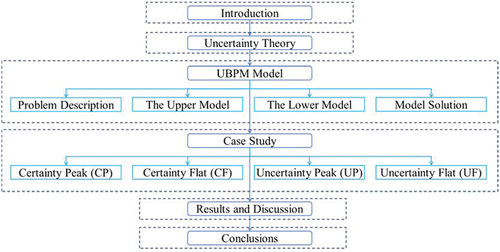
The structure of this paper is organized as follows: Section 2 introduces uncertainty theory. Section 3 establishes UBPM for hybrid vehicles. The model considered four uncertain variables including passenger arrival, passenger waiting time, interstation running time, and EBs power consumption and was solved by a genetic algorithm based on the elite strategy. Section 4 presents a case study. Section 5 shows the results and discussion. Section 6 summarizes the research conclusion. The framework of this research is shown in Figure 1.

Figure 1. The framework of this study.

Uncertainty theory

Uncertainty theory is a general term for probability theory, reliability theory, and credibility theory, as well as other theories (Peng and Liu 2002). Uncertain programming is a theoretical tool to deal with optimization problems in uncertain environments. It can be divided into three perspectives: expected value, chance measure, and chance of maximizing event realization. The expected value means that the expected value of the uncertain function is used to replace the uncertain function in the original objective function and constraint condition, respectively. The chance measure means that the decision is allowed to fail to meet the constraints to some extent. The chance of maximizing event realization means that decision-makers tend to prefer event maximization.

Concepts related to uncertainty theory

The uncertain variables in the optimization problem are divided into three categories. The following two categories are used in this article.

Expected value model (EVM)

The expected value model is based on maximizing the expectations of these uncertain objective functions under the condition that the expectation constraint is satisfied,

(1) $\left\{\begin{array}{c}maxE\left[f(x,\xi )\right]\\ subjectto:\\ E\left[g_i(x,\xi )\right]\le 0,i=1,2,\cdots ,p.\end{array}\right.$(1)

Chance constrained programming (CCP)

This uncertain programming model allows the constraint condition to be not satisfied to some extent, but the decision makes the chance of the constraint condition to be established not less than a certain confidence level. Generally, the CCP model with maximized optimism value can be expressed in the following form:

(2) $\left\{\begin{array}{c}max\bar{f}\\ subjectto:\\ Ch\{f(x,\xi )\ge \bar{f}\}\ge \beta \\ Ch\{g_i(x,\xi )\le 0,j=1,2,\cdots ,p\}\ge \alpha .\end{array}\right.$(2)

Markov process

Suppose that the number of passengers arriving is a Poisson process ($Q\left(t\right)$) with intensity $\lambda$, and each passenger’s waiting time $\left\{{\omega }_k,k=1,2,\cdots \right\}$ is independent of each other. Then, in time [0, t], the total waiting time of a bus stop is $W\left(t\right)$,

(3) $W(t)=\sum _{k=1}^{Q(t)}{\omega }_k.$(3)

The uncertain distribution of passenger waiting time

In the actual operation of the EBs, the waiting time of passengers is uncertain. It is affected by the departure interval, the volume of passengers on and off the road, and traffic conditions. Therefore, based on uncertain programming, passenger waiting time is taken as one of the uncertain variables. According to the research results of Ceder (1987), the average waiting time of passengers is

(4) $E(w)=\frac{E(H)}{2}\bullet \left[1+\frac{\mathrm{v}\mathrm{a}\mathrm{r}(H)}{E^2(H)}\right],$(4)

where $E\left(w\right)$ is the average waiting time of passengers, h;

$E\left(H\right)$ is the mean value of departure interval, h; and

$var\left(H\right)$ is the variance of departure interval, h².

The factors considered by Ceder ignore the road traffic situation and other uncertain factors. On this basis, this article integrates the uncertain distribution of passenger waiting time into a normal distribution, whose general density function and normal uncertain distribution are as follows..

(5) $\varphi (x)=\frac{1}{\sqrt{2\pi }\sigma }exp\left(-\frac{{(x-\mu )}^2}{2{\sigma }^2}\right),$(5)

(6) $\mathrm{\Phi }(x)={\left(1+exp\left(\frac{\pi (e-x)}{\sqrt{3}\sigma }\right)\right)}^{-1},x\in R.$(6)

The uncertain distribution of interstation running time

Under the influence of bus speed of the same type, the running time between bus stops can be simplified as the ratio of the distance between bus stops and the running speed of the bus. However, the actual bus running time is affected by many aspects, not only by speed, station distance, traffic lights, traffic conditions, but also by the driver, vehicle type, and so on. According to the survey data, the operating time of each station is short of the ‘Z’ uncertain distribution, and the ‘Z’ uncertain distribution is as follows:

(7) $\mathrm{\Phi }(x)=\left\{\begin{array}{c}0,ifx\le a\\ (x-a)/2(b-a),ifa\le x\le b\\ (x+c-2b)/2(c-b),ifb\le x\le c\\ 1,ifx\ge c\end{array}\right..$(7)

Uncertainty bi-level programming model

Based on the relevant knowledge of uncertainty theory in Chapter 2, UBPM is established in this part and solved by an improved genetic algorithm to achieve the goal of minimizing the total passenger travel cost and EBs energy consumption.

Problem description

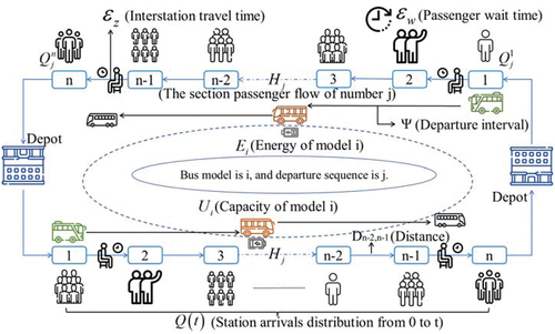
In the process of EBs operation (as shown in Figure 2), the following problems are faced. First, passengers’ waiting needs need to be satisfied. The number of passengers at each stop ($Q$) is uncertain, the waiting time for each passenger (${\epsilon }_w$) is uncertain, and the running time between each stop (${\epsilon }_z$) is uncertain. These uncertainties can cause time to increase by adding up the number of stops and the number of passengers. One of the problems to be solved in this paper is how to minimize the total expected travel time of passengers by taking the above uncertainties into account. Second, under the limited number of electric buses, the bus company considers the uncertain distribution of EBs energy consumption ($E$) with the running time, and to minimize the bus energy consumption is the second problem to be solved in this article. Finally, based on the balance of interests between bus and passengers, to minimize the passengers’ travel time and minimize the EBs energy consumption is the third problem to be solved in this paper. Since the charging of EBs is completed at the starting depot during the shift change of EBs, the charging of EBs has been considered in the vehicle scheduling in this paper. The charging method of EBs is to leave a predetermined time (10 min) at the starting depot to replace the battery. In addition, due to the battery life and long charging time, charging stations in the bus line also adopt the way of directly replacing the battery. When EBs are not in service (e.g. at night), they charge their batteries. The time and cost of a single charging task are fixed values.

Figure 2. The operation of the multi-EBs and passenger.

The UBPM provides a model basis for the study of hierarchical decision making. Suppose that a top decision maker and his subordinates have their own decision variables and objective functions. The top decision maker can influence his subordinates through his decision variables, and the subordinates have full authority to decide how to optimize their own objective functions, and these decisions will affect their respective upper leaders and subordinates. BPM focuses on feedback between layers and therefore is often accompanied by inherent uncertainty (Peng and Liu 2002),

(8) $\begin{array}{c}\left\{\begin{array}{c}\underset{x}{max}\mathrm{E}[F(x,y_1,y_2,\cdots ,y_m,\xi )]\\ subjectto:\\ E[G(x,\xi )]\le \alpha \\ \mathrm{\forall }{y}_i(i=1,2,\cdots ,m)\end{array}\right.\\ \left\{\begin{array}{c}\underset{{ }_{y_i}}{max}\mathrm{E}[f_i(x,y_1,y_2,\cdots ,y_m,\xi )]\\ subjectto:\\ \mathrm{E}[g_i(x,y_1,y_2,\cdots ,y_m,\xi )]\le \beta \end{array}\right.\end{array}.$(8)

Basic hypotheses and symbol definition

Departure interval and vehicle configuration have a comprehensive impact on the operating cost of bus companies and the total cost of passenger trips, which are the decision variables of the UBPM. However, in the actual traffic situation, there are uncertain factors such as passenger waiting time and interstation running time, which are the uncertain variables of the model. At the same time, as the decision maker, the bus company can directly change the vehicle scheduling scheme to improve the bus service level, i.e. the passengers are the upper decision makers and the bus companies are subordinates. To comprehensively consider the interests of the two parties and pursue the two objectives of the lowest cost for the bus company and the lowest total cost for passengers, a UBPM was established to solve reasonable departure interval and vehicle configuration.

Based on the following basic assumptions, UBPM is established.

Hypothesis 1: only the operation of conventional single bus lines is considered, without considering emergencies.

Hypothesis 2: passenger waiting time follows a normal distribution, and interstation running time follows ‘Z’ distribution. Passengers can wait a maximum of two times (two times, i.e. waiting for the next EBs because the EBs is currently full or for other reasons).

Hypothesis 3: only consider the operation cost of a single bus line, not considering the impact of other bus lines.

Hypothesis 4: the main factors affecting the vehicle operating cost of the bus company depend on energy consumption and maintenance costs.

Hypothesis 5: the fare for the whole journey is the same.

In the process of model building, the unified definition of the symbols used is shown in Table 1.

Table 1. Symbol definition.

Symbol	Definition	Dimension
$\mathrm{C}\mathrm{P}$	Total cost of passenger travel	yuan
$\mathrm{C}\mathrm{B}$	Total cost of EBs operation	yuan
$C_w$	Passenger waiting cost	yuan
$C_r$	Passenger travel cost	yuan
$C_s$	EBs company employee cost	yuan
$C_o$	Vehicle running cost	yuan
$C_m$	Vehicle maintenance cost	yuan
$\omega$	Waiting cost per passenger time	yuan (person min)^−1
$\mathrm{{\rm Y}}$	Travel cost per passenger time traveling	yuan (person min)^−1
${\theta }_1^i$	EBs driver cost per hour	yuan h^−1
${\theta }_2^i$	Cost per mile of public transport	yuan km^−1
${\theta }_3^i$	EBs idle cost per unit time	yuan h^−1
${\epsilon }_w$	Passenger waiting time	min
${\epsilon }_z$	Interstation travel time	min
$\psi$	Departure interval	min
$i$	EBs type	–
$x_j^i$	0–1 variable: if EBs type is i of car number j, take 1; otherwise, take 0	–
$\mathrm{n}$	Number of EBs stations	station
${\mathrm{Q}}_j^n$	The number of passengers on EBs number j at station n	person
${\mathrm{H}}_j^n$	The section passenger flow of number j from station n to n + 1	person
$\mathrm{j}$	The departure frequency	sequence•h^−1
$\mu ,\sigma$	Load factor parameters	–
$\delta$	Perception coefficient of EBs load factor	–
$U_i$	Capacity of model i	person
$u_i$	Number of seats for model i	person
$D_{n,n+1}$	Distance from station n to station n + 1	km
$T_{max}$	Maximum departure interval during investigation period	min
$T_{min}$	Minimum departure interval during investigation period	min
$maxH$	Cumulative passenger flow of maximum section	person

‘ – ’ means dimensionless.

Decision variables

Departure interval

As one of the decision variables affecting the interests of the company and passengers, the change of departure interval will cause the loss of the original balance between them. At the same time, the departure interval is also an important factor affecting passenger waiting time. Within the range of departure intervals investigated, the historical data were fitted by an uncertain normal distribution function distribution, and the following data graph was obtained, which was finally summarized in Figure 3. The impact of the departure interval on passengers’ waiting time can be clearly seen.

Figure 3. Fitting distribution of waiting time of passengers with different departure intervals.

When the departure interval is 60 min, the waiting time of passengers is concentrated in 30 min. However, when the departure interval is 6 min, the waiting time of passengers is significantly smaller, concentrated in 3 min. According to the above results, the longer the departure interval, the greater the waiting cost of passengers. On the other hand, bus companies run fewer buses, which makes them cheaper to run, but also makes them less attractive to passengers. Therefore, a reasonable design is needed to find the Pareto optimal set under the condition of meeting the needs of passengers.

Vehicle configuration

The operating speed of different EBs models has an important impact on the operating time between stations. Regardless of the impact of the traffic volume and signals on the road section, taking the Nanchang bus model as an example, they can be divided into B-type vehicles, M-type vehicles, and S-type vehicles. The buses correspond to big (B), medium (M), and small (S) EBs. The survey data are used to fit the running time between stations under different vehicle types, and the uncertainty distribution is shown in Figure 4.

Figure 4. Distribution of running time between stations of different models.

The upper model-CCP

The total passenger travel cost (CP) can be divided into passenger waiting cost (C_w) and passenger travel cost (C_r),

(9) $CP=C{\hspace{0.17em}}_w+C_r.$(9)

Passenger waiting costs

Passenger waiting cost is affected by passenger waiting time, departure interval, and number of passengers. The uncertain waiting time (${\epsilon }_w\left(\mathrm{\Psi }\right)$) and EBs departure frequency ($J$) are affected by bus departure interval and bus departure time, and the number of passengers on EBs number j at station n ($Q_j^n$) is affected by the passenger arrival rate and vehicle capacity. Taking the passenger waiting time as a normal uncertain variable, the passenger waiting cost is calculated as follows:

(10) $C_w=\omega \cdot {\epsilon }_w(\mathrm{\Psi })\cdot \sum _{j=1}^J\sum _{n=1}^{N-1}{Q}_j^n.$(10)

According to the investigation data of passenger waiting time, formula (6) is used to carry out data fitting, and when the departure interval is $\psi$, the distribution function of passenger waiting time is as formula (10),

(11) $\mathrm{\Phi }({\epsilon }_w(\mathrm{\Psi }))={\left(1+exp\left(\frac{\pi (e^{\mathrm{\Psi }}-{\epsilon }_w(\mathrm{\Psi }))}{\sqrt{3}\sigma }\right)\right)}^{-1}.$(11)

Passenger travel cost

Passenger travel cost refers to the waiting time cost of passengers taking EBs (in EBs). Passenger travel cost is not only affected by the time between stations but also the size of the car load rate will affect the psychological cost of passengers. When the car is full, the psychological time of passengers will increase. Considering the different passenger capacity of different bus models, the influence degree of load factor is also different. According to the research results of Scholar Yang, Ji, and Zhang (2015), the calculation formula of the perception coefficient (δ) of bus load factor is as follows: where $\mu =0.15,\sigma =2$. The perception coefficient of the bus load factor is the load factor value that takes into account passengers’ experience and is a multiple of the actual load factor. The greater the degree of congestion, the greater the perception coefficient,

(12) $\delta =1+\mu {\left(\frac{H_j^n}{\sum _{i=1}^I{U}_i{x}_j^i}\right)}^{\sigma }.$(12)

The running time between stations is regarded as a ‘Z’ distribution, and the passenger travel cost is calculated as follows:

(13) $C_r=\mathrm{{\rm Y}}\bullet {\epsilon }_z\left(i\right)\bullet \sum _{j=1}^J\sum _{n=1}^{N-1}\sum _{i=1}^I{\delta }_i{H}_j^n$(13)

The survey data of inter-station running time show that using formula (7) to perform data fitting, the inter-station running time distribution function of vehicle type is obtained using the following formula:

(14) $\Phi ({\epsilon }_z(i))=0,if{\epsilon }_z(i)\le a({\epsilon }_z(i)-a)/2(b-a),if\text{a}\le {\epsilon }_z(i)\le b({\epsilon }_z(i)+c-2b)/2(c-b),ifb\le {\epsilon }_z(i)\le c1,if{\epsilon }_z(i)\ge c.$(14)

Through the above formulas (9) to (14), the total travel cost of passengers can be obtained as follows:

(15) $\begin{array}{c}CP(\mathrm{\Psi },j_1,j_2,\cdots ,j_J,{\epsilon }_w,{\epsilon }_z)=\omega \cdot {\epsilon }_w(\mathrm{\Psi })\cdot \sum _{j=1}^J\sum _{n=1}^{N-1}{Q}_j^n\\ +\gamma \cdot {\epsilon }_z(i)\cdot \sum _{j=1}^J\sum _{n=1}^{N-1}\sum _{i=1}^I{\delta }_i{H}_j^n\end{array}.$(15)

The formula for calculating cross-section passenger flow is

(16) $H_j^n=H_j^{n-1}+Q_j^n-{\bar{Q}}_j^n(Droppassengerflow).$(16)

The larger the departure interval, the larger the passenger flow of a single cross-section; but since the maximum cross-section passenger flow cannot exceed the maximum capacity of the bus, the corresponding number of departures decreases, and the total cross-section passenger flow decreases. In the limited passenger capacity of each EBs, assuming that a certain section is fully loaded when passing through, its total passenger flow is the multiplication of the passenger capacity of EBs and the number of departures. Obviously, the passenger flow of the section per hour with six departures is higher than that with two departures.

Constraint conditions

① The departure interval satisfies the maximum and minimum time constraints,

(17) $T_{min}\le \mathrm{\Psi }\le T_{max}.$(17)

② Load factor formula equation requirements. Since passengers may exceed vehicle capacity during peak periods, there is a chance constraint that allows the number of passengers to exceed vehicle capacity at a confidence level. In reality, especially during rush hours, the number of passengers may exceed the capacity of the EBs. Therefore, this paper considers it as an opportunity constraint. There is a probability that the number of passengers will exceed the capacity of the EBs. This paper assumes that the number of passengers in the constraint condition is greater than the EBs capacity at the 0.95 confidence level. Therefore, the constraint equation (formula 18) is satisfied and becomes $P\left(\delta \ge 1+\mu \right)\ge 0.95$,

(18) $\delta =1+\mu {\left(H_j^n/\sum _{i=1}^I{U}_i{x}_j^i\right)}^{\sigma }.$(18)

The lower model-EVM

In the multi-model EBs operation, the total cost of EBs operation (CB) includes the staff cost of the bus company (C_s), the operating cost of different models (C_o), and the cost of idle maintenance (C_m),

(19) $CB\text{=}C{\hspace{0.17em}}_s+C_o+C_m.$(19)

Staff cost of the bus company

The staff cost of the bus company is affected by the operating time between stations and different models. The operating time between stations is an uncertain variable. For different J, the cost of the bus company is calculated as follows:

(20) $C_s=\sum _{j=1}^J\sum _{n=1}^{N-1}\sum _{i=1}^I{\theta }_1^i{\epsilon }_z^n(i)x_j^i.$(20)

Operating cost of different models

The operating cost of public transport vehicles is related to the operating mileage and vehicle types. ${\mathrm{E}}_i$ is an uncertain energy consumption distribution, which can better reflect the actual situation of battery usage. For different J values, the calculation formula is as follows:

(21) $\begin{array}{c}{C}_o=\sum _{j=1}^J\sum _{n=1}^{N-1}\sum _{i=1}^I{\theta }_2^i{D}_{n,n+1}{e}_i{x}_j^i\\ {\mathrm{E}}_i={\hat{\beta }}_{1}so{c}_{ij}^{\hspace{0.17em}}+{\hat{\beta }}_2{t}_j+{\hat{\beta }}_3{\bar{T}}_j+{\hat{\beta }}_0\end{array},$(21)

where ${\mathrm{E}}_j$ is the estimated value of the energy consumption of trip $j$, kWh; $so{c}_{ij}^{\hspace{0.17em}}$ is the state of charge at the departure time of trip $j$, %; ${\bar{T}}_j$ is the average temperature during the trip $j$,${\hspace{0.17em}}^{\circ }\mathrm{F}$; ${\hat{\beta }}_0,{\hat{\beta }}_1,{\hat{\beta }}_2,\mathrm{a}\mathrm{n}\mathrm{d}{\hat{\beta }}_3$ are regression parameters; and $e_i$ is the function of energy consumption rate of model $i$ with time (Bie et al. 2021).

Cost of idle maintenance

The daily maintenance, management, and management costs of buses are counted as idle costs per unit of time. The calculation formula is as follows:

(22) $C_m=\sum _{j=1}^J\sum _{i=1}^I{\theta }_3^i\bullet \mathrm{\Psi }\bullet (1-x_j^i).$(22)

From the above formulas (17) to (20), the total cost of bus operation is

(23) $\begin{array}{c}CB(x_j^i,j_1,j_2,\cdots ,j_J,{\epsilon }_z)=\sum _{j=1}^J\sum _{n=1}^{N-1}\sum _{i=1}^I{\theta }_1^i{\epsilon }_z^n(i)x_j^i\\ +\sum _{j=1}^J\sum _{n=1}^{N-1}\sum _{i=1}^I{\theta }_2^i{D}_{n,n+1}{e}_i{x}_j^i\\ +\sum _{j=1}^J\sum _{i=1}^I{\theta }_3^i\bullet \mathrm{\Psi }\bullet (1-x_j^i).\end{array}$(23)

Constraint conditions

① The cumulative passenger flow of the largest section of passengers satisfies the maximum and minimum constraints,

(24) $\sum _{i=1}^I{u}_i{x}_j^i\le max{\text{H}}_j^n\le \sum _{i=1}^I{U}_i{x}_j^i(\mathrm{\forall }j,n).$(24)

② 0–1 variable satisfying the statistic is 1,

(25) $\sum _{i=1}^I{x}_j^i\text{=}1.$(25)

The UBPM

Turn it into a standard UBPM as follows. First, take the optimal expectation for formula (21) and then take the optimal expectation for formula (15). The lower goal is to minimize the total cost of public transportation. The optimal number of EBs and vehicle configuration under each fixed departure interval are obtained by taking vehicle capacity and passenger demand as constraint conditions. The number of trains and vehicle configuration output by the lower target is the input of the upper target function. The upper objective is to minimize the total passenger cost and output dynamic departure intervals and vehicle sequences with service level and load factor requirements as constraints. The two decisions of this paper are the decisions of the bus company. First, bus companies minimize bus costs to determine the number of buses and vehicle configuration. Second, bus companies determine dynamic departure intervals and vehicle sequences within a day to minimize passenger costs,

(26) $\begin{array}{c}\left\{\begin{array}{c}\underset{{ }_{x_j^i}}{min}\mathrm{E}[CP(x_j^i,j_1,j_2,\cdots ,j_J,{\epsilon }_w)]\\ subjectto:\\ T_{min}\le \mathrm{\Psi }\le T_{max}\\ \delta =1+\mu {(H_j^n/\sum _{i=1}^I{U}_i{x}_j^i)}^{\sigma }\le \rho (1+\mu )\\ \mathrm{\forall }{j}_i(i=1,2,\cdots ,m)\end{array}\right.\\ \left\{\begin{array}{c}\underset{{ }_{x_g}}{min}\mathrm{E}[CB(\mathrm{\Psi },j_1,j_2,\cdots ,j_J,{\epsilon }_z)]\\ subjectto:\\ \sum _{i=1}^I{u}_i{x}_j^i\le max{\mathrm{H}}_j^n\le \sum _{i=1}^I{U}_i{x}_j^i\\ \sum _{i=1}^I{x}_j^i=1\end{array}\right.\end{array}.$(26)

The optimal EBs dispatching plan that is solved by establishing the model takes into account uncertain factors. However, in reality, the bus dispatching plan is not considered. In view of this, we take the peak period and the peace period of Nanchang public transport operation as two sets of control experiments to compare the effects of bus dispatch optimization. Taking total cost and bus line delays as evaluation indicators, the impact of uncertain factors on bus dispatching plans is analyzed.

Model solution

The basic principle of genetic algorithm is to imitate the genetic inheritance of organisms, the survival of the fittest, the less adaptable individuals are eliminated, and finally leave the more adaptable individuals, that is, the optimal solution. Because the solution is nonlinear objective programming, the genetic algorithm is suitable for solving. In the calculation process, the basic parameters are input first, and the optimal solution is obtained by using a genetic algorithm. The basic process of the genetic algorithm includes coding – population – adaptation – selection – crossover – mutation – iteration – end, as shown in Figure 5. The optimal solution is finally obtained by sorting the optimal solution.

Figure 5. Flow chart and iterative diagram of genetic algorithm.

Coding and initial

During the investigation phase, the departure interval is between 1 min and 35 min, and the departure interval is taken as an integer real number, and the binary code is used.

Fitness calculation

The fitness of the genetic algorithm is an index used to judge the pros and cons of the individuals in the group (Tan 2020). In the solution of the genetic algorithm in this paper, the maximum, minimum, and average values of each iteration are, respectively, calculated.

Selection, crossover, mutation, and elitist strategy

In the genetic process of chromosomes, excellent individuals are selected. The crossover rate is 0.8, the mutation rate is 0.1, and the elite retention rate is 0.2 so that the highly adaptable chromosomes can be copied directly to the next generation. In terms of operator selection, we use the roulette selection operator, arithmetic crossover operator, and uniform mutation operator here.

Calculate fitness again

The heredity continues, and the fitness is calculated again to generate a new population.

Iteration

Set the number of iterations to 100, 200, 300, and 400, and it has converged when the number of iterations is 400.

Output the optimal individual fitness value

The optimal departure interval was solved through genetic iterative operation, and the optimal vehicle configuration was finally determined by combining the dual uncertainty multi-objective programming model. The enumeration method was used to solve the minimum total bus cost of different vehicle configurations. After determining the minimum total bus cost, a genetic algorithm was used to solve the minimum total passenger cost of the same vehicle configuration. Finally, the optimal departure interval and vehicle configuration are solved by Pareto optimization. The results are sorted and screened to select the optimal solution of total cost.

Case study

Taking Nanchang public transportation as an example, using a genetic algorithm to solve the UBPM.

Parameter setting

According to relevant reference material (Xue et al. 2020), Nanchang urban development status, and model formula, the parameters are assigned, as shown in Table 2.

Table 2. Parameters of model.

Symbol	Definition	Dimension	Value
$\omega$	Waiting cost per passenger time	yuan (person h)^−1	50
$\mathrm{{\rm Y}}$	Traveling cost per passenger time	yuan (person h) ^−1	22
${\theta }_1^1$	B bus driver cost per hour	yuan h^−1	53
${\theta }_1^2$	M bus driver cost per hour	yuan h^−1	42
${\theta }_1^3$	S bus driver cost per hour	yuan h^−1	35
${\theta }_2^1$	B bus vehicle cost per kilometer	yuan km^−1	1.2
${\theta }_2^2$	M bus vehicle cost per kilometer	yuan km^−1	0.9
${\theta }_2^3$	S bus vehicle cost per kilometer	yuan km^−1	0.7
${\theta }_3^1$	B bus vehicle idle cost per unit time	yuan h^−1	1.15
${\theta }_3^2$	M bus vehicle idle cost per unit time	yuan• h^−1	0.92
${\theta }_3^3$	S bus vehicle idle cost per unit time	yuan h^−1	0.57
$\mu$	Load factor influence degree parameter	–	0.15
$\sigma$	Load factor influence degree parameter	–	2.00
${\delta }_1$	Influence degree of B bus load factor when full	–	1.08
${\delta }_2$	Influence degree of M bus load factor when full	–	1.11
${\delta }_3$	Influence degree of S bus load factor when full	–	1.16

Data survey

According to the survey data and historical data, the passenger flow and class volume of Nanchang Public Transport Section are shown in Table 3.

Table 3. Section passenger flow and passenger flow of Nanchang bus No. 211 in each period.

The number of station	Travel time
	9:00–10:00		17:30–18:30
	Passenger flow	Section passenger flow	Passenger flow	Section passenger flow
1	59	59	85	85
2	22		37
3	70	81	100	123
4	33	107	52	156
5	22	118	37	171
6	30	100	47	147
7	78	59	109	94
8	63	89	90	132
9	37	111	57	161
10	89	85	124	127
11	81	115	114	166
12	100	104	138	151
13	56	115	81	166
14	104	89	143	132
15	59	115	85	166
16	89	115	124	166
17	52	137	76	195
18	67	96	95	142
19	85	78	119	118
20	93	100	129	147
21	107	118	148	171
22	74	144	105	204
23	96	111	133	161
24	63	111	90	161
25	59	93	85	137
26	104	93	143	137
27	59	133	85	190
28	67	107	95	156

Solution

Based on the genetic algorithm, four different schemes are concluded: Certainty Peak (CP: red area on left), Certainty Flat (CF: green area on left), Uncertainty Peak (UP: red area on right), and Certainty Flat (UF: green area on right). The EBs scheduling arrangement is shown in Figure 6 below.

Figure 6. EBs scheduling scheme with certainty and uncertainty.

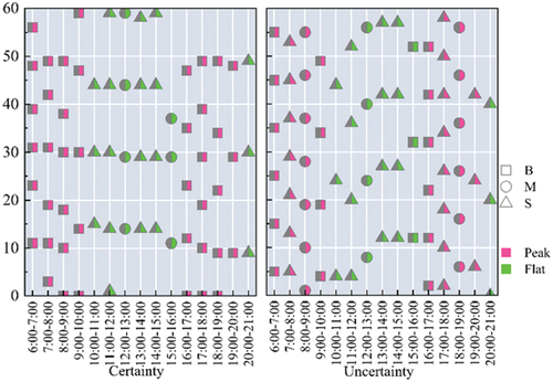
The figure on the left is the EBs scheduling scheme (CS) without considering the uncertainties, and the figure on the right is the EBs scheduling scheme (US) with the above four uncertainties taken into account. Compared with CS, US first adjusts the number of buses in different time periods. Second, different departure intervals are chosen according to passenger flow. On this basis, consider the energy consumption to select the corresponding vehicle model. During the peak period, the UP increases the number of trains than CP, i.e. it reduces the departure interval (7:00–8:00: 9.2 min-8 min). At the same time, S model and M model are adopted to reduce the cost of bus operation. Among them, model S is adopted in the period from 7:00 to 8:00, which may be because the number of passenger arrivals in this period is a discrete small aggregation peak (in a certain period, the number of passenger arrivals is smaller than the capacity of model S, i.e. the uncertain arrival distribution of passengers in a small period is considered). Compared with CF, UF adjusts M model to B model at the end of flat period, which may be to prevent the crowd gathering left over by a long idle time during flat period

Results and discussion

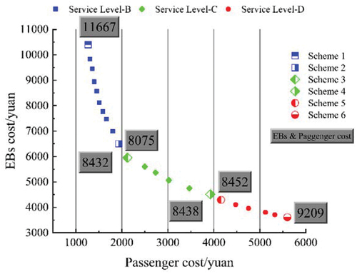
The UBPM was solved by improved genetic algorithm, and an EBs scheduling scheme considering uncertain factors was obtained. To compare the optimization effect of the scheme, the scheme was analyzed for travel time of passengers, total cost of EBs operation, and delay. In this paper, the Pareto optimal set is sorted by non-dominated order, the total cost and service level are comprehensively analyzed, and scheme 3 is selected as the final optimization scheme. Figure 7 shows the Pareto optimal solution set diagram. The horizontal axis is the total cost of passengers, and the vertical axis is the total cost of buses. Service level is divided into three levels according to the departure interval: Service level B: <10 min; Service level C: 10 ~ 20 min; Service level D: 20 ~ 30 min. The service level of Scheme 3 is C, and the total cost is the lowest.

Figure 7. Pareto optimal set and comparison between schemes.

Travel time analysis of passengers

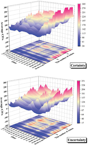
The temporal and spatial distribution of the average travel time of passengers is shown in Figure 8. The peak times are concentrated in 10:00–11:00 and 20:00–21:00, and the peak space is concentrated in 14 stations and 21 stations. The above figure now considers the uncertainties, while the following figure considers the four uncertainties proposed in this paper. Passenger travel time, the peak is lower on the lower than on the upper; In a plane projection, there are more dark blue areas (lower values) on the lower than on the upper. Through data analysis, the total passenger travel cost of the optimization scheme in this paper is reduced by 25%, which proves that considering uncertain factors can reduce the total passenger travel time.

Figure 8. The temporal and spatial distribution of average travel time of passengers.

Total cost analysis of EBs operation

Through modeling in this paper, the comparison of data before and after optimization is shown in Table 4 (The sorted result of a Pareto solution). The total cost of EBs was reduced by 8.7%, the energy consumption of EBs was reduced by 18%, and the number of EBs required was reduced by 20%. It is shown that adjusting the departure interval for different time periods can reduce the number of EBs, reduce the energy consumption, and thus reduce the cost of bus operation.

Table 4. Results of four schemes.

	Average departure interval (min)	The number of EBs	EBs cost (yuan)	Passenger cost (yuan)	Energy cost (yuan)	Average delay (s)
CP	12	26	6761	2981	3542	218
CF	15	11	4344	2463	2207	174
UP	10	20	5953	2122	3075	201
UF	17	10	4191	1925	1616	162

Delay analysis

Through sumo simulation, the delay data of EBs operation under the four schemes are output, as shown in Table 4. Total delays decreased by 7.4%, peak periods by 7.8%, and flat periods by 6.9%. It can be seen that the optimization scheme not only improves the cost of passengers and buses but also improves the efficiency of bus operation.

Conclusions

In this paper, UBPM is established by considering four uncertain variables including the number of passengers arriving, passenger waiting time, interstation running time, and EBs energy consumption. UBPM aims at minimizing the total cost of passenger travel for the upper level, and minimizing the energy consumption for the lower level. On this basis, a joint optimization strategy of dynamic departure interval and vehicle combination is proposed. The effectiveness of the proposed method is verified by an example of a real bus route. The study reached the following conclusions:

(1) There are various uncertain factors in bus operation, which affect the efficiency of bus operation. Through the uncertainty theory, the uncertainty factors can be quantitative considered, and the time and resource waste caused by the accumulation of uncertainty factors can be effectively reduced. In addition, the uncertain distribution functions of passenger waiting time and interstation running time are given.

(2) Bus scheduling optimization considering uncertain factors is beneficial to reduce the total travel time of passengers and improve the bus service level. Collaborative optimization of multiple bus models considering the fluctuation of energy consumption can meet the needs of limited bus numbers while reducing energy consumption and delay. Therefore, considering dynamic departure interval and joint optimization of multiple bus models, bus resources can be effectively integrated, and achieve the ‘Carbon Peak and Carbon Neutrality’ goals.

In this paper, only one bus route is considered, and the improvement of the model in this paper can be applied to the overall scheduling optimization of bus network routes. This paper only considers the joint optimization of the bus timetabling and vehicle scheduling in the optimization of the bus system, and the personnel scheduling will be further considered in the future. The influences of weather and ticket price are ignored in the uncertain variables considered in this paper, which will be improved in the next research.

Data availability

The data used to support the findings of this study are available from the corresponding author upon request.

Acknowledgments

This research was funded by the National Natural Science Foundation of China (No.71971005 and No. 71961006) and the Project Sponsored by Beijing Municipal Natural Science Foundation (No.8202003). These supports are gratefully acknowledged.

Disclosure statement

No potential conflict of interest was reported by the author(s).

Additional information

Funding

This work was supported by the Innovative Research Group Project of the National Natural Science Foundation of China [71971005], Innovative Research Group Project of the National Natural Science Foundation of China [71961006], and Natural Science Foundation of Beijing Municipality [8202003].

References

- Amiripour, S. M. M., A. Ceder, and A. S. Mohaymany. 2014. “Designing large-scale Bus Network with Seasonal Variations of Demand.” Transportation Research Part C-Emerging Technologies 48: 322–338. doi:10.1016/j.trc.2014.08.017.
- Baita, F., R. Pesenti, W. Ukovich, and D. Favaretto. 2000. “A Comparison of Different Solution Approaches to the Vehicle Scheduling Problem in A Practical Case.” Computers & Operations Research 27 (13): 1249–1269. doi:10.1016/s0305-0548(99)00073-8.
- Bie, Y., J. Ji, X. Wang, and X. Qu. 2021. “Optimization of Electric Bus Scheduling considering Stochastic Volatilities in Trip Travel Time and Energy Consumption.” Computer-Aided Civil and Infrastructure Engineering 36 (12): 1530–1548. doi:10.1111/mice.12684.
- Ceder, A. 1987. “Methods for Creating Bus Timetables.” Transportation Research Part a-Policy and Practice 21 (1): 59–83. doi:10.1016/0191-2607(87)90024-0.
- Ci, Y. S., Z. Y. Han, and L. N. Wu. 2021. “Bi-level Optimization Method for Urban Public Transport Regional Dispatching.” China Journal of Highway and Transport 34 (6): 196–204.
- David, B., and M. Kresz. 2020. “Multi-depot Bus Schedule Assignment with Parking and Maintenance Constraints for Intercity Transportation over a Planning Period.” Transportation Letters-the International Journal of Transportation Research 12 (1): 66–75. doi:10.1080/19427867.2018.1512216.
- Ding, P. P. 2017. “Modeling and Solving of multi-vehicle Combined Scheduling.” (Master). Zhengzhou University, Available from Cnki
- Ghaffari, A., M. Mesbah, and A. Khodaii. 2020. “Designing a Transit Priority Network under Variable Demand.” Transportation Letters-the International Journal of Transportation Research 12 (6): 429–442. doi:10.1080/19427867.2019.1629564.
- Gkiotsalitis, K. 2021. “Bus Rescheduling in Rolling Horizons for regularity-based Services.” Journal of Intelligent Transportation Systems 25 (4): 356–375. doi:10.1080/15472450.2019.1681992.
- Gkiotsalitis, K., and F. Alesiani. 2019. “Robust Timetable Optimization for Bus Lines Subject to Resource and Regulatory Constraints.” Transportation Research Part E-Logistics and Transportation Review 128: 30–51. doi:10.1016/j.tre.2019.05.016.
- Huang, Z. F., G. Ren, and H. Liu. 2013. “Optimizing Bus Frequencies under Uncertain Demand: Case Study of the Transit Network in a Developing City.” Mathematical Problems in Engineering 2013. doi:10.1155/2013/375084.
- Huang, Y., Z. W. Wang, Z. J. Li, and C. Zhu. 2016. “Coordinated Optimization of Bus and Departure Intervals in multi-vehicle Bus System.” Journal of Changsha University of Science and Technology (Natural Science) 13 (3): 37–41.
- Kulshrestha, A., Y. Lou, and Y. Yin. 2014. “Pick-up Locations and Bus Allocation for transit-based Evacuation Planning with Demand Uncertainty.” Journal of Advanced Transportation 48 (7): 721–733. doi:10.1002/atr.1221.
- Li, Z.-C., W. H. K. Lam, and S. C. Wong. 2011. “On the Allocation of New Lines in a Competitive Transit Network with Uncertain Demand and Scale Economies.” Journal of Advanced Transportation 45 (4): 233–251. doi:10.1002/atr.155.
- Li, L., H. K. Lo, W. Huang, and F. Xiao. 2021. “Mixed Bus Fleet location-routing-scheduling under Range Uncertainty.” Transportation Research Part B-Methodological 146: 155–179. doi:10.1016/j.trb.2021.02.005.
- Liu, X., and S. W. He. 2006. “Study on Bus Dispatching Model Based on dependent-chance Goal Programming.” Transport Research 12: 152–155.
- Liu, Z. G., and J. S. Shen. 2007. “Regional Bus Operation bi-level Programming Model Integrating Timetabling and Vehicle Scheduling.” Systems Engineering-Theory & Practice 11 (11): 135–141. doi:10.1016/S1874-8651(08)60071-X.
- Peng, J., and B. D. Liu. 2002. “Research Status and Development Prospect of Uncertain Planning.” Operation Research and Management 02: 1–10.
- Shen, Y., J. Xu, and J. Li. 2016. “A Probabilistic Model for Vehicle Scheduling Based on Stochastic Trip Times.” Transportation Research Part B-Methodological 85: 19–31. doi:10.1016/j.trb.2015.12.016.
- Sun, B., C. F. Yang, M. Wei, and H. Chen. 2018. “A Scheduling Model of Shuttle Buses for Stochastic Demand Passengers Based on Set Pair Analysis.” Journal of Transport Information and Safety 36 (6): 130–134.
- Tan, H. 2020. “Study on the Optimization of Bus Scheduling Based on Genetic Algorithms.” Science and Technology Innovation 32: 50–52.
- Uchida, K., A. Sumalee, and H. W. Ho. 2015. “A Stochastic Multimodal Reliable Network Design Problem under Adverse Weather Conditions.” Journal of Advanced Transportation 49 (1): 73–95. doi:10.1002/atr.1266.
- Wang, D. 2018. “Study on the Optimization Model of multi-model Configuration of Conventional Bus Lines.” (Master). Jilin University, Available from Cnki
- Wei, M. 2012. “Model and Algorithm of Regional Bus Scheduling Problem with Uncertainty Information.” (Doctorate). South China University of Technology, Available from Cnki
- Wei, M., B. Sun, and W. Z. Jin. 2013. “A bi-level Programming Model for Uncertain Regional Bus Scheduling Problems.” Journal of Transportation Systems Engineering and Information Technology 13 (4): 106–113. doi:10.1016/S1570-6672(13)60120-8.
- Xu, W. T., S. W. He, R. Song, L. Zhao, and B. S. He. 2009. “Stochastic Expected Valued Model for Multiple Bus Headways Optimization.” Transactions of Beijing Institute of Technology 29 (8): 676–680.
- Xue, Y. Q., J. Guo, J. An, L. W. Xue, and Z. Sang. 2020. “Uncertain double-decker Planning Model for Bus Line Distribution Problems.” Transportation System Engineering and Information 20 (2): 145–150.
- Yan, F., and X. P. Guang. 2008. “Model and Algorithm Analysis Based on the two-tiered Programming on Bus Scheduling.” Journal of Lanzhou Jiaotong University 27 (6): 75–79.
- Yan, S., F.-Y. Hsiao, and Y.-C. Chen. 2015. “Inter-School Bus Scheduling Under Stochastic Travel Times.” Networks & Spatial Economics 15 (4): 1049–1074. doi:10.1007/s11067-014-9280-4.
- Yan, S., and C.-H. Tang. 2008. “An Integrated Framework for Intercity Bus Scheduling under Stochastic Bus Travel Times.” Transportation Science 42 (3): 318–335. doi:10.1287/trsc.1070.0216.
- Yan, S., and C.-H. Tang. 2009. “Inter-city Bus Scheduling under Variable Market Share and Uncertain Market Demands.” Omega-International Journal of Management Science 37 (1): 178–192. doi:10.1016/j.omega.2006.11.008.
- Yang, X. Y., Y. X. Ji, and H. J. Zhang. 2015. “Perceptive Bus Dispatch Frequency and Model Optimization Models.” Journal of Tongji University (Natural Science Edition) 43 (11): 1684–1688.
- Yao, B., Q. Cao, Z. Wang, P. Hu, M. Zhang, and B. Yu. 2016. “A two-stage Heuristic Algorithm for the School Bus Routing Problem with Mixed Load Plan.” Transportation Letters-the International Journal of Transportation Research 8 (4): 205–219. doi:10.1080/19427867.2015.1110953.
- Yao, E. J., T. Liu, N. Xun, and W. F. Liu. 2020. “Regular Bus Line Departure Interval and Model Configuration Optimization.” Journal of Beijing Jiaotong University 44 (4): 86–93.
- Zhan, B., H. Y. Lu, Y. T. Yang, and R. W. Li. 2017. “Optimization of Departure Intervals considering Uncertainty of Bus Passenger Flow Demand.” Journal of Wuhan University of Technology (Transportation Science & Engineering) 41 (6): 978–983.
- Zhang, H. J., and X. P. Guang. 2014. “The Research on Model & Algorithm Based on double-deck Programming for Bus Scheduling.” Transactions of Beijing Institute of Technology 34 (1): 39–44.
- Zhang, Y., and J. F. Tang. 2014. “A risk-pooling-based Robust Model for least-time Itinerary Planning.” Journal of Transportation Systems Engineering and Information Technology 14 (4): 107–112.
- Zhang, J., D. Z. W. Wang, and M. Meng. 2020. “Optimization of Bus Stop Spacing for on-demand Public Bus Service.” Transportation Letters-the International Journal of Transportation Research 12 (5): 329–339. doi:10.1080/19427867.2019.1590677.
- Zhang, L., Z. Zeng, and K. Gao. 2022. “A bi-level Optimization Framework for Charging Station Design Problem considering Heterogeneous Charging Modes.” Journal of Intelligent and Connected Vehicles 5 (1): 8–16. doi:10.1108/JICV-07-2021-0009.
- Zhang, W. W., H. Zhao, and M. Xu. 2021. “Optimal Operating Strategy of Short Turning Lines for the Battery Electric Bus System.” Communications in Transportation Research 1: 100023. doi:10.1016/j.commtr.2021.100023.