Detection and analysis of transfer time in urban rail transit system using WIFI data

ABSTRACT

This study presents a comprehensive framework for estimating passengers' transfer times and extracting their distribution and related transfer routes using WIFI probe data. The departure time of preceding station, arrival time of subsequent station, and train running time are selected to obtain transfer times. Then, the collected data is analyzed using kernel density estimation to obtain candidate distribution. Gaussian mixture models are adopted to extract the distribution of each possible transfer route at both peak hours and off-peak hours. This method is tested at two transfer stations of Xi’an metro system with the comparison of results from automatic fare collection data and manual sampling survey data. The results indicate that the proposed approach can collect the transfer time with a sampling ratio greater than 30% and a deviation less than 5%. The route choice behaviors and distribution of transfer time under various conditions can be identified using the proposed methods.

KEYWORDS:

• Transfer time
• distribution and changing trend
• Urban Rail Transit System
• route choice behaviors
• Gaussian mixture model
• WIFI probe data

Introduction

Backgrounds

The transfer stations in urban rail transit system (URTS) service passengers that both arrive at and depart from the station and those who transfer to another line. The facilities in the transfer stations may experience a low level of service when the arrival passengers and transfer passengers wait for the coming train at the same time (Elhamshary et al. 2019). The interarrival times of passengers entering any metro station can be considered as a random arrival process. While, the arrivals of transfer passengers are a highly predictable intermittent process, which relates to train schedule (Xu et al. 2014). The transfer time is the duration that transfer passengers will stay in the transfer station, which is the summation of transfer walking time from preceding metro line to subsequent one and dwell time. The dwell time is duration from the time arriving waiting platform to the time of train departure. If the system operators can be provided with the real-time transfer time and its distribution, train schedule and route guidance/control measures at the transfer stations can be adjusted to improve operation efficiency by minimizing both transfer walking time and dwell time (Sun et al. 2014).

Transfer time exhibits high variability (Chang 2010) and uncertainty (Aguiléra et al. 2014) in URTS operation due to unexpected crowding (Helbing et al. 2005) and/or complicated designs of the facilities (Ye et al. 2008). Such variability and uncertainty not only reduce the passengers’ comfort but also deteriorate the performance of URTS (Hänseler, Bierlaire, and Scarinci 2016). The identification of transfer times and determination of their distributions can provide the operators and authorities with information on congestion level, route choices, and a better understanding of capacities (Li, Zhang, and Nan et al. 2018).

Measuring the transfer time automatically with high accuracy is always challenging at URTS. The data collection can be accomplished using either automatic sensors or manual collection method. When the automatic sensing methods are utilized, more advanced algorithms are needed to extract the potential characteristics or changing patterns from the raw data. The manual data collection method can be designed to address the problem directly but have a low sampling ratio. All existing data sources, such as the automatic fare collection (AFC) data (Sun and Xu 2012), the location-based data provided by the GPS (Vij and Shankari 2015) or cellular network (Carrel et al. 2015), WIFI probe (Gu et al. 2020a, 2020b), and the manually collected data from selected participants (Gu et al. 2017; Du, Liu, and Liu 2009), can be utilized to identify specific passenger behaviors in various range and accuracy. However, an effective method with related automatic data collection technology is still needed to identify real-time transfer time and its changing pattern under a complicated transfer environment with reasonable accuracy and efficiency (Zhao et al. 2016). Although manual collection methods are considered as the most effective method to obtain transfer time, there still exist biases within the sample data because of the low sampling ratio (Hong et al. 2017).

With recent advances in low-cost sensing technologies (Li et al. 2019), more data can be obtained to improve the accuracy of transfer time estimation, such as the train dynamic provided by the accelerometer, the location-based information collected from the fixed Bluetooth (Li and Souleyrette 2016) or WIFI sensors (Gu et al. 2020a, 2020b), and other environmental information (Gu et al. 2017). The WIFI sensors can provide passengers’ location-based information with a sampling ratio greater than 30% (Li, Zhang, and Nan et al. 2018), which is more adequate than Bluetooth (less than 5% (Li and Souleyrette 2016)). Therefore, a reliable WIFI-based sensing system with corresponding algorithms is needed to automatically monitor transfer time and extract its features.

Literature review

The transfer time can be measured using manual or automatic methods. Data collected by manual surveys can be either filed data or from carry-on sensors. Fixed sensors, such as AFC, location-based (e.g., base station) mobile signaling data, and video camera, are the most dominant data source for the determination of transfer time. Extra algorithms are needed for extracting required features.

Measuring transfer times of all passengers manually is a time-consuming and trivial task. Manual measuring methods need the investigators to record the actions of specific passengers manually or using carry-on sensors. Most studies require the investigators to record what the transfer passengers did during the transfer process (Gu et al. 2017; Du, Liu, and Liu 2009). In order to access precise passenger actions at the transfer stations, some experiments request the investigators to repeat the passengers’ actions exactly, which can be recorded by the carry-on sensors on themselves. Because the sampling ratio of manual survey method is limited, sampling expansion and pattern recognition algorithms are commonly used when these methods are selected. However, transfer time may be affected by excessive delays caused by traffic demand or flow control measures (Wales and Marinov 2015). With these delays, passengers may miss the next train and must wait at the platform (Fan, Guthrie, and Levinson 2016), which increases the transfer time. If the data collection process doesn’t cover these situations, the detected results will be no longer reliable.

Fixed detectors have difficulties in tracing the spatio-temporal trajectories of the transfer passengers. A unique identification with related timestamps will be needed to track studied subject between detectors. Then, the trajectory can be identified by connecting the positions of detected sensors in chronological order. AFC data is the most easily accessible data source to extract the macroscopic spatial distribution of trips (Kieu, Bhaskar, and Chung 2015; Zhang and Yao 2015), such as OD matrix (Zhao, Rahbee, and Wilson 2007), route choices (Zhou, Shi, and Xu 2015), and trip purpose (Lee and Hickman 2014). Because AFC data only records the origin and destination of a specific trip, it is difficult to identify passengers’ actions within URTS. Mobile signaling data is another good source for location-based identification (Aguiléra et al. 2014). The signaling data of mobile device is highly dependent on the locations of base stations, which may be not suitable to determine transfer times. What’s more, the signaling data has the privacy problem, making it very difficult to obtain for conventional research. Although the image recognition technologies (Zhou, Chen, and Yang et al. 2014) can also be utilized to determine transfer route and walking time between cameras, it is difficult to cover every passenger in the platform to determine dwell time. Meantime, the identification of every passenger between cameras is also time-consuming and inefficient, which is difficult to be done in real time. Instead of passengers themselves, their locations can be determined by locating the items carried by them in a noncontact way, such as wireless transmission via Bluetooth and WIFI (Carrel et al. 2015; Gu et al. 2020a; Li and Souleyrette 2016; Dunlap et al. 2016). Compared with the low sampling ratio of Bluetooth, which is less than 5%, WIFI-based information provides a promising alternative data source with a sampling ratio of more than 30%. Either Bluetooth data or WIFI data needs additional algorithms to determine the distribution and trend of transfer times.

When the manual method is employed to acquire the transfer time, the results need to be expanded and calibrated using statistical methods. The sampling expansion algorithms usually belong to Bayesian statistical methods, which use manually collected data as a priori probability (Jang 2010). The most commonly utilized algorithms include random walk/forest with Naïve Bayes classifier or Markov chain Monte Carlo (MCMC) (Ma, Wu, and Wang et al. 2013). With the expanded sample data, either histogram or kernel density estimation (KDE) (He and Trépanier 2015) can be used to obtain the numerical solution of the probability density function. The maximum likelihood method or the least square method (Hou and Xu 2012) can be utilized to test fitness between a proposed distribution and observed probability density.

Besides simulation models (Hassannayebi et al. 2020), pattern recognition methods offer an effective way to extract potential characteristics from a large field data set (Li, Zhao, and Li 2019), such as transfer time data obtained from automatic sensors. When sufficient samples are provided, the possible distribution of transfer times under various traffic demand or passenger flow control measures is the most effective information for URTS operators (Yu et al. 2014). The estimation of probability distribution can start with creating a histogram from the samples. When the shape of the histogram matches a predefined probability distribution, the parametric density estimation method can obtain the unknown parameters of the selected distribution. Nonparametric density estimation will be applied in the situation with no candidate distribution. The KDE method can plot the shape of probability density without giving a probability function. In most time, it is difficult to use a simple probability distribution to represent the precise transfer features. This situation is mainly caused by mixing multiple transfer choices, for instance, a transfer station with multiple transfer routes. Unsupervised clustering algorithms can be selected to distinguish these transfer choices, which include linear discriminant analysis (Krygsman, Dijst, and Arentze 2004), artificial neural network (Garrido, De Oña, and De Oña 2014), support vector machine (Yu et al. 2017), and decision tree (Hernandez, Monzon, and de Oña 2016). Typical applications of unsupervised algorithms on similar problems include the usage of principal components analysis (Lois, Monzón, and Hernández 2018), random forests (Gal et al. 2017), and K-means clustering (Zhang et al. 2019). Semi-supervised methods may be a better choice when a small amount of labeled data is available. Existing work indicates the transductive support vector machine (Keerthi and Lin 2003), and Gaussian mixture model (GMM) (Li and Zhao 2019) can be used to recognize hidden features from a large amount of traffic data.

In general, an effective way to collect and identify the transfer time and its changing patterns with adequate accuracy is still urgently needed. Existing research gaps can be summarized as follows.

1. Necessary data needed for the identification and characterization of transfer time can either be manually or automatically collected. The manually collected data can be fine-grained for precise actions of passengers but limited in the term of sample size. While, methods using automatically collected data sources still have accuracy and/or efficiency issues. Thus, it is reasonable to develop an automatic data collection and processing method so as to obtain transfer times and related properties.

2. Transfer times under homologous environments appear to have similar changing patterns in the form of distribution. Existing researches mainly focus on the description of data but ignore the distinctive changing patterns of transfer time under various conditions. Identification and estimation method to extract and distinguish changing patterns of transfer times under various traffic and management measures is urgently needed.

Objective and contributions

The objective of this study is to develop robust sensing and pattern recognition methods to identify transfer times at the transfer station of URTS. The major contributions of this study are twofold: (1) An automatic transfer time detection system for URTS is proposed using distributed WIFI sensors installed at preceding and subsequent stations to avoid interferences on detection at the transfer station. The transfer times and related route selection behaviors can be detected with acceptable reliability and accuracy. (2) A comprehensive model using GMM is proposed to extract underlying distributions of transfer time under various traffic demands, passenger flow control measures, and facility designs, which can provide references on developing precise management measures.

The remainder of this paper is organized as follows. Section II describes the proposed system, data collection, and the method to calculate transfer time. The recognition method using the GMM and MCMC method to identify the distributions of transfer times at all possible scenarios is illustrated in Section III. Section IV verifies the proposed methods using data from Xi’an metro system. The main findings are listed in Section V.

Transfer time detection

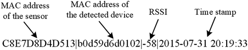
Any network device will constantly broadcast the “probe” information when its WIFI function is enabled, which can be named as “WIFI devices.” A WIFI sensing system is developed to capture this “probe” information, which includes the Media Access Control (MAC) address, the Received Signal Strength Indication (RSSI), and the timestamp. Figure 1 illustrates the probe data format. The WIFI sensing system can be named as “sensing devices,” which is essentially a wireless router without a broadcasting function. It only scans the probe information for every second within its detection range, which can be gained by an antenna. If the sensing devices are installed at the platform level, the arrival time and departure time of detected devices can be obtained by extracting the first and last timestamp of one specific MAC address.

Figure 1. Components of one sample probe frame.

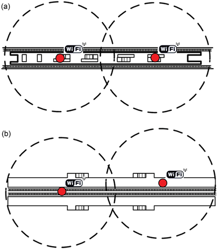
Because the theoretical sensing range is a circle (Porter et al. 2013), the sensing devices are recommended to be installed along the central line of the roof at the platform level to achieve a better coverage. The antenna shall be placed vertically to guarantee the coverage on both sides is the same. At this time, the horizontal detection range is approximately a circle (Baccour et al. 2012). If the detected RSSI from WIFI device is higher than a predefined threshold, it can be considered that this WIFI device is in the detection range of sensing device. Because no data communication between the sensing device and WIFI device is needed during the process of collecting probe information, the threshold can be slightly lower than minimal RSSI needed for data transmission, which is around −80dbm~−90dBm (Porter et al. 2013; Baccour et al. 2012). In this study, the threshold is chosen as −100 dBm. Based on field tests at a crowded platform, the position with an RSSI of −100 dBm is approximately 35 meters from the sensing device. Thus, 35 meters is selected as the detection range.

As shown in Figure 2, the installation locations of sensing devices are different between the stations with an island platform and side platforms. Two sensing devices can provide sufficient coverage of the platform designed for a train with six type-B cars (single car length is 19 meters), and three devices can service the train with eight type-A cars (single car length is 22 meters). More sensing devices may be needed if the station has a special layout design. When a specific WIFI device is detected by multiple sensing devices at the same time, data with the highest RSSI will be selected.

Figure 2. Device installations on various types of urban rail transit stations. (a) Island type platform. (b) Side type platforms.

The departure time of preceding station and arrival time of subsequent station are selected to estimate transfer time, including transfer walking time and dwell time. As travel time between stations is known in URTS, the transfer time I can be calculated by Equation (1)(1) $I=A_d-D_u-T$(1) .

(1) $I=A_d-D_u-T$(1)

where, A_d is the arrival time of subsequent station, D_u is the departure time of preceding station, and T is the total travel time between preceding and subsequent stations by the train.

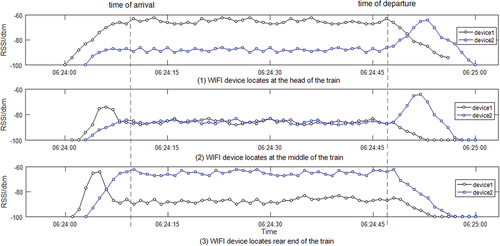
Based on the relative position between sensing devices and WIFI device, the detected probe information may represent various variation trends during the process of train arriving and departing. The departure and arrival time, as well as the location of WIFI devices, can be detected based on the variations of detected RSSI. In the case of trains with six type-B cars, there will be two sensing devices installed. The WIFI devices can be located either between or on the other side of these two sensing devices. As illustrated in Figure 3, the RSSI of detected WIFI devices on the train will represent three patterns. The arrival time and departure time can be determined when the variations of detected RSSIs are smaller than 10 dBm, which is common fluctuation of RSSI during train dwelling process.

Figure 3. Patterns of the probe information at the station with two sensors.

Another threshold will be needed to avoid the situation of multiple detections of one particular WIFI device, e.g., round trips. This threshold can be determined based on the common transfer time of a specific transfer station. Any detected transfer time that longer than this threshold will be considered as two separate trips.

Characteristics of transfer time

Framework

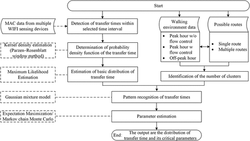
The proposed solution framework is outlined in Figure 4. The number of clusters and the basic distribution of transfer times are needed in the pattern recognition algorithm. Because transfer time in different routes and walking environments will represent differentiated features in the form of distribution, we make the number of clusters be the product of the number of routes and walking environments. The traffic demand and passenger flow control measures are considered as the mainly influence factors of walking environments. The basic distribution of transfer time can be estimated using maximum likelihood estimation. The candidate distribution used in the maximum likelihood estimation can be obtained by observing the probability density estimated by KDE method, such as the Parzen–Rosenblatt window method (Han et al. 2018). When number of clusters for possible distributions of transfer time is determined, the parameters of each distribution can be estimated by GMM, which can be solved using expectation maximization (EM) algorithm. When the sampling rate is not enough, the MCMC can be used to generate random samples according to the data distribution obtained by GMM.

Figure 4. Framework of pattern recognition on transfer time.

Identification of cluster number

The transfer times are mainly attributed to walking environments and route choices. Thus, we can assume the number of clusters for transfer time be the combinations of all possible contributing attributes. A transfer station with a complicated design can have multiple routes to change from one metro line to another. Each route corresponds to the possible walking environments, which are related to demands. Besides the categories of walking environments between peak hours and off-peak hours, the passenger flow control measures will turn the walking environment into another. Passenger flow control measures can increase the capacity of transfer route by increasing total walking distance, which will cause excessive delays. Thus, it can only be applied to heavy demand conditions. Considering all influence factors, each route can be presented with three classifications, which are peak hour with/without passenger flow control measures and off-peak hour.

Determination of basic distribution

The KDE method (Han et al. 2018), which is a nonparametric method, was selected to estimate the probability density of transfer time. The KDE method estimates the probability density of a specific point based on a finite data sample. The bandwidth and kernel are two critical parameters in KDE. Assume x_n is the nth measured transfer time. Let (x₁, x₂, …, x_n) be a univariate independent and identically distributed sample of transfer time with a predefined time window. Its probability density $\hat{f}$ can be estimated by the kernel density estimator shown in Equation (2)(2) ${\hat{f}}_h(x)=\frac{1}{n}\sum _{i=1}^n{K}_h(x-x_i)=\frac{1}{nh}\sum _{i=1}^n{K}_h(\frac{x-x_i}{h})$(2) . The bandwidth h was determined with considerations between the bias of estimator and its variance, which was mainly related to the time granularity selected in the estimation. For the optimal combination of hyperparameters, cross-validation method was implemented to determine the optimal bandwidth.

(2) ${\hat{f}}_h(x)=\frac{1}{n}\sum _{i=1}^n{K}_h(x-x_i)=\frac{1}{nh}\sum _{i=1}^n{K}_h(\frac{x-x_i}{h})$(2)

where K is the kernel, which is a non-negative function; h is the bandwidth, which is the smoothing parameter that should be greater than 0; K_h(x) = h⁻¹ K(x/h) is the scaled kernel, which is a kernel with subscript h.

Although the KDE method can obtain the approximate estimation of probability density at any specific point, the basic distribution of transfer time remains unknown. At this time, the transfer times under a specific condition can be utilized to obtain its basic distribution. Maximum likelihood estimation method is selected to fit field-collected data to the proposed distributions. The proposed distribution with the highest coefficient of determination (R²) will be considered as the basic distribution of transfer time under that predefined condition.

Pattern recognition

The GMM was selected to extract the distributions of transfer time under each condition. Transfer time data captured by sensing devices was aggregated. With basic distribution and number of clusters, the GMM is capable to identify each distribution by fitting with finite Gaussian distributions. Thus, when each distribution of all generated data points follows a Gaussian or Gaussian related distribution (such as the logarithmic Gaussian distribution), GMM will be the best way to estimate the unknown parameters for each distribution. The parameters of proposed GMMs can be derived using EM algorithm with the data from sensing devices. When the selected time interval is small with insufficient samples, the parameters of GMM can be obtained using Bayesian-based MCMC algorithm (Dias and Wedel 2004) with the well-trained prior model.

Assume the random variable of transfer time is x, its GMM p(x) can be expressed by Equation (3)(3) $p(x|\pi ,\mu ,{\sigma }^2)=\sum _{k=1}^K{\pi }_{k}N(x|{\mu }_k,{\sigma }_k^2)$(3) . Let z be a latent variable, z_k can be either 0 or 1 and $\sum _K{z}_k=1$. When z_k = 1, it means the kth component is selected, i.e. $p(z_k=1)={\pi }_k$. At this time, the selected transfer time is clustered into the kth cluster. If z_k is an independent and identically distributed random variable, the prior probability can be given by Equation (4)(4) $P(z)=p(z_1)p(z_2)\cdots p(z_K)=\prod _{k=1}^K{\pi }_k^{z_k}$(4) . When the kth component follows a Gaussian distribution, the likelihood probability is shown in Equation (5)(5) $P(x|z)=\sum _{k=1}^{K}N{(x|{\mu }_k,{\sigma }_k^2)}^{z_k}$(5) . Then, posterior probability can be obtained by combining Equations (4)(4) $P(z)=p(z_1)p(z_2)\cdots p(z_K)=\prod _{k=1}^K{\pi }_k^{z_k}$(4) and (5(5) $P(x|z)=\sum _{k=1}^{K}N{(x|{\mu }_k,{\sigma }_k^2)}^{z_k}$(5) ), which is illustrated in Equation (6)(6) $\gamma (z_k)=p(z|x)=\frac{{\pi }_k\cdot N(x|{\mu }_k,{\sigma }_k^2)}{\sum _{j=1}^K{\pi }_j\cdot N(x|{\mu }_j,{\sigma }_j^2)}$(6) .

(3) $p(x|\pi ,\mu ,{\sigma }^2)=\sum _{k=1}^K{\pi }_{k}N(x|{\mu }_k,{\sigma }_k^2)$(3)

Where, π_k is the mixture coefficient, $\sum _{k=1}^K{\pi }_k=1$,$0\le {\pi }_k\le 1$; $N(x|{\mu }_k,{\sigma }_k^2)$ is the kth component of the mixture model, and ${\mu }_k,{\sigma }_k^2$ are the mean value and variance of the kth component.

(4) $P(z)=p(z_1)p(z_2)\cdots p(z_K)=\prod _{k=1}^K{\pi }_k^{z_k}$(4)

(5) $P(x|z)=\sum _{k=1}^{K}N{(x|{\mu }_k,{\sigma }_k^2)}^{z_k}$(5)

(6) $\gamma (z_k)=p(z|x)=\frac{{\pi }_k\cdot N(x|{\mu }_k,{\sigma }_k^2)}{\sum _{j=1}^K{\pi }_j\cdot N(x|{\mu }_j,{\sigma }_j^2)}$(6)

Case study and verification

Experiment design and data characteristics

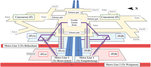
The Beidajie station, which is the transfer station of line 1 and line 2 of the Xi’an Metro system, was selected as a testbed. As shown in Figure 5, this station is an underground station with three levels. Line 1 lies at the −2 floor with two side type platforms, and line 2 lies at the −3 floor with an island type platform. There are two routes between every transfer direction. For example, passengers who transfer from line 2 to line 1(Houweizhai) can use the route of (train → −3 F side A → −2 F side A) or route (train → −3 F side B → −2 F side B → −1 F → −2 F side A). Some passengers who are unfamiliar with the design of station may choose the longer route. The passenger flow control measures will be applied at the concourse level when the high demand occurs. Under the passenger flow control measures, the passenger must make a detour with a lower walking speed.

Figure 5. Layout and transfer routes of the Beidajie station.

Ten sensing devices were installed at four stations linked to Beidajie station. The Zhonglou station has a special design to protect the historical relics near the station. Therefore, two additional sensing devices were installed to ensure the coverage of WIFI devices. The experiment was carried from Oct 15^th, 2016 to Oct 29^th, 2016. We chose one weekday data (Oct 19^th, 2016) to analyze the sampling ratio. 151,628 matched samples (the sample number of passengers with transfers was 74,443) were collected on that day. Based on the AFC data of the same date set, the sampling ratios for all passengers and the ones with transfers were 31.66% and 32.99%, respectively. The average sampling ratio during the 2-week experiment was 32.86%. Manually collected data on the same day was selected to verify the proposed methods.

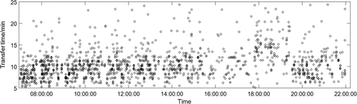
All transfer times of all routes detected by sensing devices are illustrated in Figure 6. The data before 7:00 was removed to eliminate the influences caused by the unbalanced arrival time of the first few trains in both directions. The passenger flow control measures were applied at the concourse level from 18:00 to 19:30. The transfer times in Figure 6 indicate that excessive delays were caused during the period with passenger flow control measures.

Figure 6. Variations of detected transfer time.

The manual investigation method was also implemented to verify the proposed method. Ten investigators were employed to record the critical time stamps of the transfer passengers during the transfer process. The selected time stamps include the alighting time, boarding time, walking time, and dwell time, which can be used to calculate the transfer time of this passenger. The investigated passengers were selected randomly. 739 effective samples were collected. The description and comparison between these two data sets are introduced in the next section.

Descriptions of WIFI-based transfer time

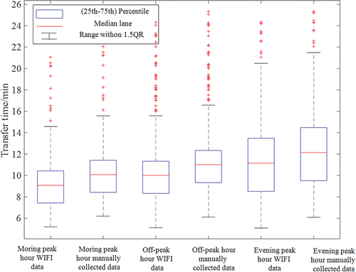
Based on the number of transfer route and traffic demand of Beidajie station, the transfer times for one transfer direction of one day represented six states: morning peak hour (2 routes, without passenger flow control measures, 7:00–9:00), off-peak hour (2 routes) and evening peak hour (2 routes, with passenger flow control measures, 18:00–19:30). Figure 7 shows the statistical characteristics of the transfer times in these six states based on manually collected data. The results indicate that the transfer time for some routes (such as train → −3 F side B → −2 F side B → −1 F → −2 F side A) were significantly higher than others (like train → −3 F side A → −2 F side A). The transfer times with passenger flow control measures were higher than those without the measures. Figure 8 shows comparisons between the proposed method and manual investigation. The comparisons on mean and variances showed a deviation that less than 5%. The mean value of WIFI-based data was approximately 36 seconds less than the manually collected data. It was probably because the sampling ratio of manually collected data is biased.

Figure 7. Comparison of transfer time between routes 1 and 2 at Beidajie station.

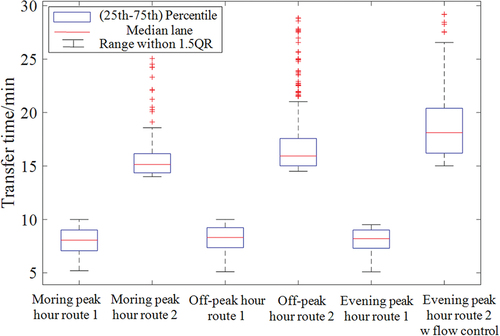
Figure 8. Comparison of transfer time characteristics estimated based on manually collected data and WIFI data.

To minimize deviation caused by route selection, we chose data collected in Xiaozhai station, where all the transfer directions have only one route, to estimate the distribution of probability density. The fitting results of peak hours and off-peak hours using KDE and maximum likelihood estimation are shown in Figure 9. The normal distribution, lognormal distribution, Weibull distribution, and Gamma distribution were selected as candidate distributions. The fitting results of maximum likelihood estimation showed that normal distribution and lognormal distribution had the coefficient of determinations (R²) greater than 0.9, which are better than Weibull distribution and Gamma distribution. The estimated parameters for normal distribution and lognormal distribution are listed in Table 1. Therefore, the transfer time for a specific route follows the Gaussian distribution.

Figure 9. Analysis of the probability density of transfer time.

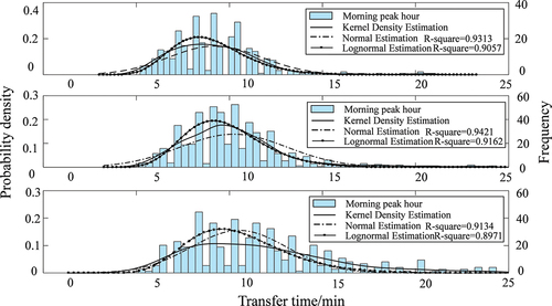
Table 1. Estimated parameters of the proposed distributions.

	Normal distribution			Lognormal distribution
Parameters Period	Morning peak	Off-peak	Evening peak	Morning peak	Off-peak	Evening peak
μ	9.233	10.224	11.612	2.190	2.290	2.401
σ^2	2.500	2.879	3.837	0.251	0.258	0.316
R^2	0.931	0.942	0.913	0.906	0.916	0.897

Changing patterns of transfer time

As shown in Table 1, although the R² of normal distributions have a high value, the data distributions are left-skewed, which indicates the lognormal distribution is a better option. Thus, both normal distribution and lognormal distribution are selected as the base function in the GMM to estimate the parameters of these fitting functions. The EM algorithm was selected to estimate the parameters GMM. The number of Gaussian/lognormal distributions was 6, the number of iterations was 10 and the convergence accuracy was 10⁻⁴. Figure 10 shows the pattern recognition results of raw data in Figure 6 using GMMs with both normal distribution and lognormal distribution as the base functions. The parameters of each Gaussian distribution and the statistical parameters of corresponding manual collected data are listed in Table 2. The results of both GMM models show a good ability to determine the pattern of transfer time. Both models can distinguish the transfer time into morning/evening peak hours and off-peak hours. The differences of these two models mainly exist in the abnormal long transfer time, which represent a relatively high variance. The Kolmogorov–Smirnov test gives a p-value of 0.3505, which indicates there is no difference between these two data samples. The distribution parameters obtained from GMM can be used as the priori probability in further estimation of transfer time.

Figure 10. Extracted patterns of transfer time by GMM. (a) Estimation using GMM with normal distribution as base function. (b) Estimation using GMM with lognormal distribution as base function.

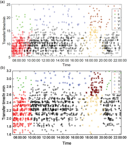
Table 2. Comparisons between parameters of GMM and manually collected data.

State	State I		State II		State III		State IV		State V		State VI
Parameter	μ1	σ1	μ2	σ2	μ3	σ3	μ4	σ4	μ5	σ5	μ6	σ6
GMM/Normal	8.725	2.857	17.047	2.533	9.353	2.434	18.761	2.000	9.595	2.753	19.995	2.568
GMM/Lognormal	2.151	0.049	2.349	0.023	2.212	0.076	2.674	0.039	2.257	0.053	2.960	0.020
Manual	7.827	1.183	16.174	2.249	8.192	2.117	16.882	2.952	8.902	1.049	18.842	3.298

Discussion

The transfer time and its possible distribution at URTS can be determined using the proposed method. However, there are still some fluctuations on the detected results. Besides the contributing factors considered in the proposed models, the differences in the headways of the related metro lines can also be a contributing factor. A simplified scenario can be utilized to analyze the effect of headway on transfer time. Assume all passenger’s walking times are the same, the transfer time will represent a periodic change, which will increase to a specific value gradually, then directly return to the original value after a few time intervals. Take the situation of Beidajie station as an example, the headways of line 1 and line 2 were 295 seconds and 223 seconds, respectively. It is assumed all the walking times of passengers from line 2 to line 1 were 300 seconds, and all passengers waiting at the platform can abroad the train. At this time, the dwell time will be 72 seconds longer than it is of the previous train until it is greater than 295 seconds. Because the detected transfer times from the sensing devices will be the result of combined effects from all contributing factors and the walking speed of transfer passengers varies, it is difficult to obtain the distribution and changing pattern of transfer time directly. The extra waiting time caused by the differences of headways of two metro lines explains the patterns obtained by sensing devices. The proposed method has the ability to minimize this influence by extracting the distribution of sample data set. However, the model can still be improved with the considerations of differences in headways when the headways are known.

In this study, the transfer times were divided into six clusters, meaning six kinds of passenger behaviors. Clusters I, III, and V represented the transfer route with short walking distance, while the rest clusters corresponded to complicated transfer behaviors, which may take the longer route. The results indicated that the transfer times in the morning peak hour were shorter than other periods. One possible reason for this phenomenon is the headway of both lines at the peak hour is about 15% shorter than it is at the off-peak hour. A lower headway will result in a shorter dwell time, thus the transfer times in the morning peak hour were shorter. More passengers have a longer transfer time in the evening peak hour than the morning peak hour and off-peak hour. This phenomenon indicated that passengers that chose the route that passes through the concourse level were significantly affected by the flow control measures.

If the studied time selected to capture potential features of transfer times is relatively small, the sample size used in the proposed methods maybe not enough. At this time, the GMM using MCMC sampling can be utilized to acquire the characteristics of transfer times. The estimated parameters of each Gaussian model can be treated as the properties of the selected studied time, which can be used for the predictions of transfer times.

Conclusions

An automatic method using WIFI probe information is proposed to identify the transfer time in URTS with an adequate sampling ratio. Furthermore, a GMM with EM/MCMC estimation is established to extract complicated transfer behaviors under various traffic and management states from the collected data set.

The proposed transfer time detection method is able to accurately and automatically identify the transfer time at a complex metro transfer station. The comparison between manually investigated data and collected data indicates that the proposed method can yield robust and accurate estimation results, leading to only 5% or less deviation.

The results of GMM based algorithm indicate that the transfer times at Xi’an metro system are normal or lognormal distributed and can be clustered based on traffic demand and passenger flow control measures. The passengers’ route choice behaviors and distribution of the transfer time can be determined from collected WIFI probe data.

This study focuses on the detection of transfer times at the transfer station of URTS using WIFI probe information. Although the sampling ratio is higher than other data sources and distributions of transfer time can be extracted using GMM, there are still certain deviations between the observed data and predicted data. One possible reason is that one passenger may carry multiple WIFI devices, which results in overestimation. Another possible reason might be that the signal strength can be affected by the crowd. Future work needs to further improve the detection accuracy and predict the transfer time using existing information for possible application on URTS management.

Disclosure statement

No potential conflict of interest was reported by the author(s).

Additional information

Funding

This work is jointly supported by the National Natural Science Foundation of China under Grant [number 51408049] and the Natural Science Basic Research Plan in Shaanxi Province of China under Grant [number 2020JM-237].

References

- Aguiléra, V., S. Allio, V. Benezech, F. Combes, and C. Milion. 2014. “Using Cell Phone Data to Measure Quality of Service and Passenger Flows of Paris Transit System”. Transportation Research Part C: Emerging Technologies 43: 198–211. doi:10.1016/j.trc.2013.11.007.
- Baccour, N., A. Koubaa, L. Mottola, M. A. Zúñiga, H. Youssef, C. A. Boano, M. Alves, et al. 2012. “Radio Link Quality Estimation in Wireless Sensor Networks: A Survey.” ACM Transactions on Sensor Networks 8 (4): 1–35. doi:10.1145/2240116.2240123.
- Carrel, A., P. S. Lau, R. G. Mishalani, R. Sengupta, and J. L. Walker. 2015. “Quantifying Transit Travel Experiences from the Users’ Perspective with High-Resolution Smartphone and Vehicle Location Data: Methodologies, Validation, and Example Analyses”. Transportation Research Part C: Emerging Technologies 58: 224–239. doi:10.1016/j.trc.2015.03.021.
- Chang, J. S. 2010. “Assessing Travel Time Reliability in Transport Appraisal.” Journal of Transport Geography 18 (3): 419–425. doi:10.1016/j.jtrangeo.2009.06.012.
- Dias, J. G., and M. Wedel. 2004. “An Empirical Comparison of EM, SEM and MCMC Performance for Problematic Gaussian Mixture Likelihoods.” Statistics and Computing 14 (4): 323–332. doi:10.1023/B:STCO.0000039481.32211.5a.
- Du, P., C. Liu, and Z. Liu. 2009. “Walking Time Modeling on Transfer Pedestrians in Subway Passages.” Journal of Transportation Systems Engineering and Information Technology 9 (4): 103–109. doi:10.1016/S1570-6672(08)60075-6.
- Dunlap, M., Z. Li, K. Henrickson, and Y. Wang. 2016. “Estimation of Origin and Destination Information from Bluetooth and Wi-Fi Sensing for Transit.” Transportation Research Record 2595 (1): 11–17. doi:10.3141/2595-02.
- Elhamshary, M., M. Youssef, A. Uchiyama, A. Hiromori, H. Yamaguchi, and T. Higashino. 2019. “Crowdmeter: Gauging Congestion Level in Railway Stations Using Smartphones”. Pervasive and Mobile Computing 58: 101014. doi:10.1016/j.pmcj.2019.04.005.
- Fan, Y., A. Guthrie, and D. Levinson. 2016. “Waiting Time Perceptions at Transit Stops and Stations: Effects of Basic Amenities, Gender, and Security.” Transportation Research Part A: Policy and Practice 88: 251–264.
- Gal, A., A. Mandelbaum, F. Schnitzler, A. Senderovich, and M. Weidlich. 2017. “Traveling Time Prediction in Scheduled Transportation with Journey Segments”. Information Systems 64: 266–280. doi:10.1016/j.is.2015.12.001.
- Garrido, C., R. De Oña, and J. De Oña. 2014. “Neural Networks for Analyzing Service Quality in Public Transportation.” Expert Systems with Applications 41 (15): 6830–6838. doi:10.1016/j.eswa.2014.04.045.
- Gu, W., K. Zhang, Z. Zhou, M. Jin, Y. Zhou, X. Liu, C. J. Spanos, et al. 2017. “Measuring Fine-Grained Metro Interchange Time Via Smartphones”. Transportation Research Part C: Emerging Technologies 81: 153–171. doi:10.1016/j.trc.2017.05.014.
- Gu, J., Z. Jiang, W. D. Fan, J. Wu, and J. Chen. 2020a. “Real-Time Passenger Flow Anomaly Detection considering Typical Time Series Clustered Characteristics at Metro Stations.” Journal of Transportation Engineering, Part A: Systems 146 (4): 04020015. doi:10.1061/JTEPBS.0000333.
- Gu, J., Z. Jiang, Y. Sun, M. Zhou, S. Liao, and J. Chen. 2020b. “Spatio-temporal Trajectory Estimation Based on Incomplete Wi-Fi Probe Data in Urban Rail Transit Network”. Knowledge-Based Systems 211: 106528. doi:10.1016/j.knosys.2020.106528.
- Han, W., W. Wang, X. Li, and J. Xi. 2018. “Statistical-Based Approach for Driving Style Recognition Using Bayesian Probability with Kernel Density Estimation.” IET Intelligent Transport Systems 13 (1): 22–30. doi:10.1049/iet-its.2017.0379.
- Hänseler, F. S., M. Bierlaire, and R. Scarinci. 2016. “Assessing the Usage and Level-of-Service of Pedestrian Facilities in Train Stations: A Swiss Case Study.” Transportation Research Part A: Policy and Practice 89: 106–123.
- Hassannayebi, E., M. Memarpour, S. Mardani, M. Shakibayifar, I. Bakhshayeshi, and S. Espahbod. 2020. “A Hybrid Simulation Model of Passenger Emergency Evacuation under Disruption Scenarios: A Case Study of A Large Transfer Railway Station.” Journal of Simulation 14 (3): 204–228. doi:10.1080/17477778.2019.1664267.
- He, L., and M. Trépanier. 2015. “Estimating the Destination of Unlinked Trips in Transit Smart Card Fare Data.” Transportation Research Record 2535 (1): 97–104. doi:10.3141/2535-11.
- Helbing, D., L. Buzna, A. Johansson, and T. Werner. 2005. “Self-Organized Pedestrian Crowd Dynamics: Experiments, Simulations, and Design Solutions.” Transportation Science 39 (1): 1–24. doi:10.1287/trsc.1040.0108.
- Hernandez, S., A. Monzon, and R. de Oña. 2016. “Urban Transport Interchanges: A Methodology for Evaluating Perceived Quality.” Transportation Research Part A: Policy and Practice 84: 31–43.
- Hong, L., Y. Yan, M. Ouyang, H. Tian, and X. He. 2017. “Vulnerability Effects of Passengers’ Intermodal Transfer Distance Preference and Subway Expansion on Complementary Urban Public Transportation Systems”. Reliability Engineering & System Safety 158: 58–72. doi:10.1016/j.ress.2016.10.001.
- Hou, F., and R. H. Xu. 2012. “Model of Passenger Flow Assignment for Urban Rail Transit Based on Entry and Exit Time Constraints.” Transportation Research Record 2284 (1): 57–61. doi:10.3141/2284-07.
- Jang, W. 2010. “Travel Time and Transfer Analysis Using Transit Smart Card Data.” Transportation Research Record 2144 (1): 142–149. doi:10.3141/2144-16.
- Keerthi, S. S., and C.-J. Lin. 2003. “Asymptotic Behaviors of Support Vector Machines with Gaussian Kernel.” Neural Computation 15 (7): 1667–1689. doi:10.1162/089976603321891855.
- Kieu, L. M., A. Bhaskar, and E. Chung. 2015. “A Modified Density-Based Scanning Algorithm with Noise for Spatial Travel Pattern Analysis from Smart Card AFC Data.” Transportation Research Part C: Emerging Technologies 58: 193–207. doi:10.1016/j.trc.2015.03.033.
- Krygsman, S., M. Dijst, and T. Arentze. 2004. “Multimodal Public Transport: An Analysis of Travel Time Elements and the Interconnectivity Ratio.” Transport Policy 11 (3): 265–275. doi:10.1016/j.tranpol.2003.12.001.
- Lee, S. G., and M. Hickman. 2014. “Trip Purpose Inference Using Automated Fare Collection Data.” Public Transport 6 (1–2): 1–20. doi:10.1007/s12469-013-0077-5.
- Li, P., and R. R. Souleyrette. 2016. “A Generic Approach to Estimate Freeway Traffic Time Using Vehicle Id‐Matching Technologies.” Computer-Aided Civil and Infrastructure Engineering 31 (5): 351–365. doi:10.1111/mice.12159.
- Li, Y., K. Zhang, S. Nan, K. Chen. 2018. “Identification of Trip Characteristics in Urban Rail Transit System Using Distributed Trip Information.” Journal of Transport Information and Safety 36 (1): 96–102.
- Li, D., and Y. Zhao. 2019. “A Multi-Categorical Probabilistic Approach for Short-Term Bike Sharing Usage Prediction.” IEEE Access 7: 81364–81369. doi:10.1109/ACCESS.2019.2923766.
- Li, D., Y. Zhao, and Y. Li. 2019. “Time-Series Representation and Clustering Approaches for Sharing Bike Usage Mining.” IEEE Access 7: 177856–177863. doi:10.1109/ACCESS.2019.2958378.
- Li, Y., F. Wang, H. Ke, -L.-L. Wang, and -C.-C. Xu. 2019. “A Driver’s Physiology Sensor-Based Driving Risk Prediction Method for Lane-Changing Process Using Hidden Markov Model.” Sensors 19 (12): 2670. doi:10.3390/s19122670.
- Lois, D., A. Monzón, and S. Hernández. 2018. “Analysis of Satisfaction Factors at Urban Transport Interchanges: Measuring Travellers’ Attitudes to Information, Security and Waiting.” Transport Policy 67: 49–56. doi:10.1016/j.tranpol.2017.04.004.
- Ma, X., Y. J. Wu, Y. Wang, F. Chen, J. Liu. 2013. “Mining Smart Card Data for Transit Riders’ Travel Patterns”. Transportation Research Part C: Emerging Technologies 36: 1–12. doi:10.1016/j.trc.2013.07.010.
- Porter, J. D., D. S. Kim, M. E. Magaña, P. Poocharoen, and C. A. G. Arriaga. 2013. “Antenna Characterization for Bluetooth-Based Travel Time Data Collection.” Journal of Intelligent Transportation Systems 17 (2): 142–151. doi:10.1080/15472450.2012.696452.
- Sun, Y., and R. Xu. 2012. “Rail Transit Travel Time Reliability and Estimation of Passenger Route Choice Behavior: Analysis Using Automatic Fare Collection Data.” Transportation Research Record 2275 (1): 58–67. doi:10.3141/2275-07.
- Sun, L., J. G. Jin, D. H. Lee, K. W. Axhausen, and A. Erath. 2014. “Demand-Driven Timetable Design for Metro Services”. Transportation Research Part C: Emerging Technologies 46: 284–299. doi:10.1016/j.trc.2014.06.003.
- Vij, A., and K. Shankari. 2015. “When Is Big Data Big Enough? Implications of Using GPS-Based Surveys for Travel Demand Analysis.” Transportation Research Part C: Emerging Technologies 56: 446–462. doi:10.1016/j.trc.2015.04.025.
- Wales, J., and M. Marinov. 2015. “Analysis of Delays and Delay Mitigation on a Metropolitan Rail Network Using Event Based Simulation.” Simulation Modelling Practice and Theory 52: 52–77. doi:10.1016/j.simpat.2015.01.002.
- Xu, X., J. Liu, H. Li, and J.-Q. Hu. 2014. “Analysis of Subway Station Capacity with the Use of Queueing Theory”. Transportation Research Part C: Emerging Technologies 38: 28–43. doi:10.1016/j.trc.2013.10.010.
- Ye, J., X. Chen, C. Yang, and J. Wu. 2008. “Walking Behavior and Pedestrian Flow Characteristics for Different Types of Walking Facilities.” Transportation Research Record 2048 (1): 43–51. doi:10.3141/2048-06.
- Yu, K., H. Zhu, H. Cao, B. Zhang, E. Chen, J. Tian, J. Rao, et al. 2014. “Learning to Detect Subway Arrivals for Passengers on a Train.” Frontiers of Computer Science 8 (2): 316–329. doi:10.1007/s11704-014-3258-8.
- Yu, H., Z. Wu, S. Wang, Y. Wang, and X. Ma. 2017. “Spatiotemporal Recurrent Convolutional Networks for Traffic Prediction in Transportation Networks.” Sensors 17 (7): 1501. doi:10.3390/s17071501.
- Zhang, Y. S., and E. J. Yao. 2015. “Splitting Travel Time Based on AFC Data: Estimating Walking, Waiting, Transfer, and in-Vehicle Travel Times in Metro System.” Discrete Dynamics in Nature and Society 2015: 539756. doi:10.1155/2015/539756.
- Zhang, X., Y. Zheng, L. Sun, and Q. Dai. 2019. “Urban Structure, Subway Systemand Housing Price: Evidence from Beijing and Hangzhou, China.” Sustainability 11 (3): 669. doi:10.3390/su11030669.
- Zhao, J., A. Rahbee, and N. H. Wilson. 2007. “Estimating a Rail Passenger Trip Origin‐Destination Matrix Using Automatic Data Collection Systems.” Computer-Aided Civil and Infrastructure Engineering 22 (5): 376–387. doi:10.1111/j.1467-8667.2007.00494.x.
- Zhao, J., F. Zhang, L. Tu, C. Xu, D. Shen, C. Tian, X.-Y. Li, et al. 2016. “Estimation of Passenger Route Choice Pattern Using Smart Card Data for Complex Metro Systems.” IEEE Transactions on Intelligent Transportation Systems 18 (4): 790–801. doi:10.1109/TITS.2016.2587864.
- Zhou, J. B., H. Chen, J. Yang, J. Yan. 2014. “Pedestrian Evacuation Time Model for Urban Metro Hubs Based on Multiple Video Sequences Data.” Mathematical Problems in Engineering 2014:843096.
- Zhou, F., J.-G. Shi, and R.-H. Xu. 2015. “Estimation Method of Path-Selecting Proportion for Urban Rail Transit Based on AFC Data.” Mathematical Problems in Engineering 2015: 350397. doi:10.1155/2015/350397.