Regional non-CO₂ greenhouse gas fluxes inferred from atmospheric measurements in Ontario, Canada

Abstract

Independent verification of bottom-up greenhouse gas (GHG) emission inventories is crucial for a reliable reporting of Kyoto gases to the United Nations Framework Convention on Climate Change. Here, we use a pseudo-data experiment to test if our improved version of the well-known Radon tracer method (RTM) is able to quantitatively retrieve regional GHG fluxes. Using in-situ observations in Egbert, Canada, from 2006 to 2009 for the RTM, we derive night-time fluxes of CH₄ and N₂O in southern Ontario. The N₂O fluxes found have a inter-quartile range of 7.6–31.2 μgN₂O/(m²h) with an overall mean of 24.4 ± 5.6 μgN₂O/(m²h). Comparison with the EDGAR4.1 inventory revealed an underestimation by a factor of 1.7 ± 0.4 in the inventory, which is explainable by missing natural sources and a missing seasonal cycle in the inventory. Our RTM-based fluxes of CH₄ with a inter-quartiles range of 0.19–0.49 mgCH₄/(m²h) and a mean of 0.36 ± 0.08 mgCH₄/(m²h) lie significantly below the inventory-based estimates of 0.79 ± 0.06 mgCH₄/(m²h). Using a Stochastic Time-Inverted Lagrangian Transport (STILT) model this difference can be attributed to an overestimation of CH₄ emissions in a specific region, the highly urbanized Greater Toronto Area. This study displays how the application of the RTM in future monitoring networks could help to assess high-resolution emission inventories.

Keywords:

• non-CO₂ greenhouse gases
• regional flux estimate
• Radon
• top-down
• urban emissions

1. Introduction

Since industrialization human activities have influenced our environment and already started to alter it in many ways. Prominently, the increase of the atmospheric greenhouse gases (GHGs) burden is the largest anthropogenic contribution to the additional radiative forcing that mainly drives climate change (IPCC 2007). Among the GHGs, CO₂ is the most important one, causing an additional radiative forcing of 1.66 W/m². The non-CO₂ GHGs also add a significant amount of about 1 W/m² (IPCC 2007). Especially, CH₄ and N₂O notably account for 0.48 W/m² and 0.16 W/m², respectively (IPCC 2007) because the atmospheric mixing ratios of CH₄ and N₂O were also substantially altered since pre-industrial times from a global average of 715 ppb to more than 1774 ppb in the case of CH₄ and from 270 to more than 319 ppb in 2005 for N₂O (IPCC 2007). To stop future increases of their atmospheric mixing ratios the emission of GHGs are now subject to international regulatory treaties, e.g. the Kyoto-Protocol, that aim to limit the human influence on climate. Their emissions are therefore reported to the United Nation Framework Convention on Climate Change (UNFCCC). The emission compilation though solely relies on national bottom-up emission statistics provided by the individual member states. The annual mean emissions for CO₂ are usually reported to have an uncertainty of about 10–40% for national totals (NRC 2010; Peylin et al. 2011). Compiling proper emission inventories for CH₄ and N₂O is even more complex and the emission inventories are thus often reported to be more uncertain (Olivier et al. 1999; Jonas et al. 2010; NRC 2010). For the latter gases emission inventories commonly have to apply a parameterization to estimate emissions using mean emission ratios for e.g. CH₄/CO₂ in different processes (IER 2009), which usually have large uncertainties. Furthermore, the emissions of e.g. N₂O can be delayed, which means that they are not immediate and include biochemical reactions in the soils. To be able to assess the available emission inventories top-down approaches are an independent and valuable tool (Nisbet and Weiss 2010). Commonly, large-scale atmospheric inversion studies are performed. Although large uncertainties (still) adhere to top-down estimates, their results can help to confirm given inventories, but sometimes also raise questions about the limitations of deriving temporally and spatially highly resolved emission inventories solely using bottom-up approaches.

Bergamaschi et al. (2010), for example found noticeable differences of about 40% between the top-down flux estimates of CH₄ over the European continent compared to the bottom-up inventories. For North America, where the CH₄ concentrations are subject to a larger influence from biogenic sources, inversion studies found noticeable deviations of the prior CH₄ fluxes ranging from −17% to +9% (Bousquet et al. 2006; Pison et al. 2009), but could not attribute this to a specific emission sector. Understanding especially the anthropogenic CH₄ emissions is crucial as they currently account for 2/3 of the global annual source (IPCC 2007). Within the anthropogenic share, emissions from the agricultural sector account for about 50% of the fluxes, with the other major constituents being fugitive emissions from fossil fuel production and landfills.

For N₂O a recent global inversion indicated that the anthropogenic emissions are underestimated by about 20% (Corazza et al. 2011). Regional scale studies found that their estimates agreed within about 30% with emissions reported to UNFCCC for the investigated domain of Northern Europe (Ryall et al. 2001; Manning et al. 2003). For N₂O the anthropogenic share is also a significant part of the global budget accounting for about 45% mostly from agriculture (fertilized soil ≈25%, cattle ≈13%) and fossil fuel burning (≈8%) (Montzka et al. 2011). Besides the large-scale inversions, other studies, purely based on experimental data, focus on the regional and local scale using the Radon tracer method (RTM) (Levin et al. 1999). Those studies mainly conducted in Europe helped to assess the available emission maps on a small-scale and to detect long-term trends in the local fluxes (Schmidt et al. 2001; Messager et al. 2008; Levin et al. 2011).

This study aims at quantifying the fluxes on a limited spatial domain in North America. For the first time fluxes of CH₄ and N₂O in Southern Ontario, a major industrial center of Canada, are derived solely from atmospheric observations. Our Egbert site has a unique location at the borderline of the highly populated Greater Toronto Area (GTA) and the regions of Ontario that are dominated by agriculture contrasted by the sparsely populated northern part of Ontario. This allows quantifying the GHG fluxes in these important regions using an independent top-down approach. We utilize an enhanced version of the established RTM to derive local fluxes, which are then compared with flux estimates from a fine-grained emission inventory i.e. EDGAR V4.1 (EDGAR 2010). Using the Stochastic Time-Inverted Lagrangian Transport (STILT) model (Lin et al. 2003) for a pseudo-data experiment we further investigate if the RTM is able to resolve the spatially varying GHGs fluxes of the emission map. Lastly, we use the spatial information of our model to investigate the difference of the observed and inventory-based fluxes in order to attribute it to specific regions and emitter groups.

2. Methods

2.1. Measurements of GHG and Radon

The measurements were performed at the Center for Atmospheric REsearch (CARE) of Environment Canada in Egbert, Ontario (44.23°N, 79.78°W). In the south-easterly direction of the site, large anthropogenic emissions are generated in the so-called “Golden Horseshoe” area with a population of approximately 8.1 million people, including the highly urbanized GTA inhabited by 5.5 million people (StatsCan 2008). Ontario also comprises a significant agricultural industry with farmlands on an area of 53,860 km², including 36,600 km² crops, as well as a livestock of 1,800,000 cattle and 300,000 sheep. Our measurement site is placed at the borderline of these regions and thus is influenced from urban as well as agricultural and sparsely populated areas.

2.1.1. Trace gas measurements

The CH₄ and N₂O measurements used in this study were performed quasi-continuously (hourly) using a HP6890II gas chromatograph (Hewlett-Packard) equipped with a flame ionization detector (FID) to analyze CH₄ and an electron capture detector (ECD) to quantify N₂O; a detailed description of the analytical system can be found in Worthy (2003). The air intake was at a height of 10 m above ground initially at the “clean-air building” and was moved to an adjacent tower (to a distance of about 100m) with a height of 25 m in 2009. For the CARE site no significant local sources of CH₄ and N₂O are present. The quality of the in-situ dataset is assured by comparison to bi-weekly grab samples. The reproducibility of CH₄ and N₂O mole fractions was determined for similar setups to be 0.1 ± 2.5 ppb for CH₄ and 0.03 ± 0.34 ppb for N₂O. To assure the compatibility of the Greenhouse Gases Monitoring Laboratory (GGML) measurements, frequent inter-laboratory comparison measurements are performed and have shown the reliability of the used protocols (Worthy 2003).

2.1.2. Radon measurements

Measurement of the atmospheric ²²²Radon daughter activity is co-located with the GHG measurement; the Heidelberg Radon-Monitor setup was used (Levin et al. 2002). The ²²²Radon activity concentration is calculated from the measured activity of its daughter ²¹⁴Po that is attached to aerosols and collected on a static filter. ²¹⁴Po decay on the filter is monitored with a commercial Canberra PIPS 900 AM detector from a solid angle of 0.265 assuming 100% efficiency of the detector. For our measurements, we only use integrated hourly activities and apply a semi-empiric disequilibrium factor of 1.367 (Levin et al. 2002).

2.2. Radon tracer method

To be able to infer fluxes f_i from the given concentration time series of CH₄ and N₂O we use a simple box model for the atmospheric boundary layer. We assume that the boundary layer is a laterally homogeneous, well-mixed box with only a temporally varying vertical height h(t). Thus, the concentration change in this box equals the flux of the tracer i through the box boundaries, scaled by the box volume:

Equation (1) is true for all conservative tracers, i.e. tracers that have no (significant) sink within our spatio-temporal domain. Applying Equation (1) for two different tracers which have a similar spatial distribution and temporal variation of emissions, we can assume that both the mixing height h(t) as well as the area A(t) is the same. We thus derive:

A technique using the measurements of concentrations of the investigated tracer i and Radon as tracer j with the given known Radon flux f_j is the so-called RTM. When using ²²²Rn as a tracer, its radioactive decay has to be corrected for, which we do following Schmidt et al. (2001). The RTM has been applied in various studies investigating e.g. CH₄, N₂O, and H₂ fluxes (Levin et al. 1999; Schmidt et al. 2001; Hammer and Levin 2009). These studies often focus on the fluxes of GHG during the night-time when enhanced thermal cooling of the ground causes boundary layer inversions and suppressed vertical mixing. In these situations the night-time boundary layer is shallow leading to pronounced temporal concentration changes dc_i /dt for all trace gases having significant sources or sinks. For this type of flux estimations ²²²Radon is an especially suitable tracer as it is emitted continuously from the soil, and its radioactive half-life of 3.824 days prevents the buildup of large background activities. In the RTM, we assume that the ²²²Rn-flux does not significantly vary within the night.

Our algorithm already applied in Hammer and Levin (2009) goes beyond this well-known model by introducing different selection criteria to ensure that the results are physically meaningful. The following constraints have been introduced into the selection process. (i) Both the Radon as well as the tracer time series must have a linear correlation with time, which implies (quasi-) constant fluxes and a stable boundary layer height. (ii) A minimum threshold for the increase of the concentration of the tracer and Radon. By setting a minimal increase we make sure that the slope is larger than the detection limit given by the individual measurement errors. Furthermore, (iii) the selection rejects situations where the concentration increase lasts longer than the defined time window of our night-time inversion situation, to avoid interpreting increases due to synoptic events, i.e. lateral transport of polluted air to our site. Therefore, we can assure that the signals interpreted are dominated by the local fluxes. A crucial modification was (iv) that the algorithm uses an advanced linear regression routine (Krystek and Anton 2007) that includes an exact analytical solution to regression problems including uncertainties for both x and y values. Finally, (v) the fitting algorithm has the ability to automatically flag outliers in the observation record to ensure robustness of the estimate. In order to estimate absolute CH₄ and N₂O fluxes we need to know the ²²²Radon exhalation rate in the local catchment area. We use the Radon flux data climatology from Schery and Wasiolek (1998) for our domain in Canada and the United States, applying their seasonal (i.e. monthly) emission factors. This datasets has previously been used in modeling studies and been shown to agree well with observational data and new maps on global and regional scale (Griffiths et al. 2010; Hirao et al. 2010). Recently, a global modeling study (Zhang et al. 2011) that included more highly resolved Radon flux maps from Szegvary et al. (2009), used the Schery and Wasiolek (1998) map for the parts of the globe not covered by these high resolution maps (e.g. Canada), found good agreement of model prediction and observed concentrations. We assessed the seasonal and inter-annual variability of the ²²²Rn fluxes in our domain using gamma dosimetry data from eight sites of the fix surveillance network of Health Canada in southern Ontario ( http://www.hc-sc.gc.ca/ewh-semt/contaminants/radiation/surveill/data-donnees/index-eng.php). The variation of this proxy is driven by the variations of the ²²²Rn fluxes (Szegvary et al. 2007, 2009). We find that the seasonal cycle of our inventory is in line with the observed seasonal variability and only small inter-annual variabilities of 5–15% of the monthly means. For our estimation of the uncertainty in the ²²²Rn flux we decided to be conservative and used the largest difference we could find, i.e. 25% (February 2008 to February 2009) which was due to significantly different snow cover.

2.3. Bottom-up estimates

The bottom-up emission estimates of CH₄ and N₂O are available from the EDGAR V4.1 inventory (EDGAR 2010) on a 0.1° × 0.1° global map and the annual emission data is provided sector-specific. To be able to compare the bottom-up inventory with the top-down RTM flux estimates, we have to account for atmospheric mixing as different grid cells of the bottom-up inventory influence our air mass depending on the meteorological conditions. To account for that we use an influence function I_x,y (t). This influence function gives the weighting coefficients for the flux of every grid cell g_x,y to calculate the resulting mean flux F(t).

The influence function is calculated using the STILT (Lin et al. 2003). We also derive the commonly used so-called footprint (Gerbig et al. 2003), which is the result of integrating the influence function in space and time for each time step. The STILT model is driven by meteorology from the Eta Data Assimilation System (EDAS) of the Air Research Laboratory (ARL) of the National Oceanic and Atmospheric Administration (NOAA) (ftp://arlftp.arlhq.noaa.gov/pub/archives/edas40/) with a spatial resolution of 40 km by 40 km and a three-hourly temporal resolution. The limited temporal resolution might lead to problems when comparing the modeling results with observational data, as they might lag in properly representing (rapid) changes by up to three hours. To derive the hourly resolution time-series, the three-hourly wind fields were interpolated and the fluxes included using a footprint emission linker after aggregating the footprint to match the gridded 0.1° × 0.1° resolution of the EDGAR V4.1 emission inventory.

3. Results and discussion

3.1. Pseudo-data experiment to test the RTM

To investigate the applicability of the RTM and to be able to confidently interpret our top-down flux estimates we use our modeling framework for a pseudo-data experiment for 2005. We want to especially test if the RTM is able to retrieve fluxes quantitatively and uncover biases associated with this method. We thus simulated concentration time-series for CH₄, N₂O, and Rn in Egbert. Fluxes of CH₄ and N₂O were taken from the annually constant EDGAR V4.1 inventory (EDGAR 2010) and Rn fluxes were used from the Schery and Wasiolek (1998) map at monthly resolution. The atmospheric transport was modeled with the STILT model (Lin et al. 2003) in the configuration described in section 2.3.

As observational data is subject to measurement uncertainty, another simulation was run that included the given uncertainties, i.e. 2.5 ppb for CH₄ and 0.34 ppb for N₂O. For the RTM we selected the night-time from 22:00 h to 06:00 h local time and all other parameters and thresholds described in section 2.2 for our retrieval. The retrieval results are then compared with the initial input fluxes, i.e. our inventory fluxes weighted according to the modeled footprints. A key problem for comparing the RTM fluxes over the given window from 22:00 h to 06:00 h to the hourly fluxes of the emission model was that the RTM did not always include all measurement values within this time window due to, e.g. bad correlation between Radon and the trace gas. As these measurements do not fulfill the requirements to be included in the RTM they are flagged and not accounted for in the flux estimate. Instead, we use aggregated three-hourly fluxes from the emission model during night to compare with if less than one point was flagged out in this period. Given that the meteorological data has a quite limited temporal resolution (three-hourly) we occasionally encounter timing problems of the meteorological fields. We therefore compare our RTM fluxes for the 22:00 h–06:00 h window with the modeled 22:00 h–06:00 h, 20:00 h–04:00 h, and 24:00 h–08:00 h averaged fluxes and choose the best match in this window. The contribution to the total flux from each grid cell of the inventory is given by the normalized footprints.

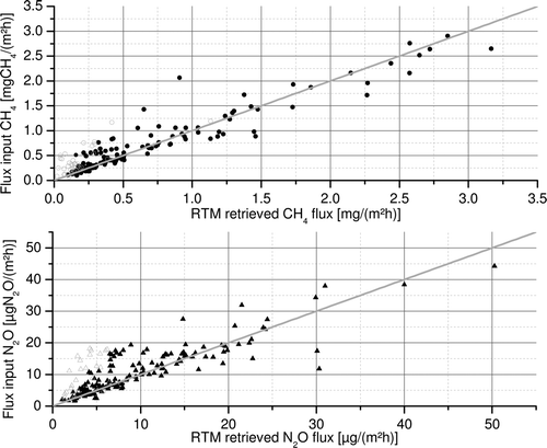
We find that the retrieved RTM fluxes are in good agreement with the bottom-up estimates for both CH₄, as well as N₂O, see Figure 1. They generally follow the 1:1 line and the retrieved means of 0.70 ± 0.06 mgCH₄/(m²h) (SD 0.67 mgCH₄/(m²h)) for CH₄ and 9.8 ± 0.5 μgN₂O/(m²h) (SD 7.8μg N₂O/(m²h)) for N₂O compare well with the mean of the initial fluxes of 0.73 ± 0.06 mgCH₄/(m²h) (SD 0.63 mgCH₄/(m²h)) for CH₄ and 10.8 ± 0.6 μgN₂O/(m²h) (SD 7.8 μgN₂O/(m²h)) for N₂O, respectively. Nevertheless, the RTM seems to underestimate certain situations in the lower concentration range for both tracers to some extent (open gray circles). This could be attributed to conditions when the footprint and thus the mean GHG fluxes of our domain vary strongly during the retrieval period. During these situations the relation between the concentration changes dc_tracer and dc_radon becomes non-linear; this behavior could be used to identify those situations in the post-processing. Nevertheless it seems that some situations where this occurs might have remained in the dataset, thus RTM results from observational data have to be selected carefully and could be slightly biased to lower values in general. Still the fluxes derived from the in-situ measurement time-series should be well compatible to the real fluxes. We furthermore find that only for about 15% of the days in our pseudo-data record a meaningful flux can be derived using the RTM (using a threshold of R = 0.8 for the correlation of Rn and CH₄ or N₂O during night-time). The RTM flux data coverage is also seasonally varying with sparse coverage in winter and more successful retrieval of fluxes in spring, summer, and fall. In winter the concentration variations are mainly driven by synoptic air mass changes rather than displaying the distinct diurnal cycles of the mole fractions that are needed to apply the RTM. This selective sampling could of course introduce a bias when comparing them to mean annual fluxes. We find that the mean flux of CH₄ derived by the RTM of 0.70 ± 0.06 mg/(m²h) still only differs by 4% from the night-time mean of all hourly fluxes of 0.73 ± 0.02. The N₂O annual mean night-time flux in our catchment area of 13.2 ± 0.8 is, however underestimated by 25%. This difference could be explained by the seasonally varying catchment area and the fact that the spatial distribution of N₂O emission is less homogeneous than the CH₄ emissions. We conclude that comparing the sporadic night-time data to simple annual means is especially challenging for N₂O fluxes in our domain. Thus, when comparing observation and inventory fluxes we have to make sure that only the fluxes of the nights included in the RTM (i.e. fulfill the RTM selection criteria) are accounted for in the inventory-based flux estimate. Overall our pseudo-data experiment displays that there are certain limitations to the RTM results but that it is in general a valuable approach to assess the overall level of fluxes. One has to be aware though, that generalizing our pseudo-data experiment results to observational data relies on the models ability to realistically model atmospheric transport. As the STILT model has been investigated and characterized in numerous studies, we only performed a simple test to check if it can realistically reproduce the mean diurnal cycle of the mixing ratios of atmospheric trace gases, which is utilized for the RTM. We found that the modeled and the observed mean diurnal cycle of the Radon concentrations agree within 35% for the summer (JJA) 2006. Given that a significant share of this difference could be due to the uncertainty of the ²²²Rn flux (c.f. section 2.2.) our modeling setup appears to be appropriate. We thus conclude from our pseudo-data experiment, that the RTM (when combined with a modeling study) can be used to assess the regional GHG flux and possibly monitor long-term changes if the seasonal Radon fluxes as well as its inter-annual changes are well-known.

Figure 1. Comparison of initial fluxes and the RTM retrieved fluxes for CH₄ (upper panel) and N₂O (lower panel). The 1:1 line is given in gray. Open gray symbols denote flux estimates that were rejected due to a strongly varying flux during night-time.

3.2. CH₄ fluxes in Southern Ontario derived from in-situ observations using the RTM

After analyzing the RTM algorithm with the pseudo-data experiment, we have a good basis to interpret the results of the in-situ data from Egbert, Ontario. We used the hourly in-situ observations within the time window from 22:00 h to 06:00 h local time to infer the night-time CH₄ fluxes. A total of 133 nights from 2006 to the end of 2009 fulfill the selection criteria of the RTM, this corresponds to about 10%, as expected (Hammer and Levin 2009). We furthermore find that the data coverage is similar to our simulation being especially sparse in winter, (see Figure 2; upper panel). The observed CH₄ flux estimates’ inter-quartile range spans from 0.19 to 0.49 mgCH₄/(m²h). The inter-quartiles range for the emission inventory-based estimates are considerably larger, i.e. 0.41 to 0.92 mgCH₄/(m²h). The observational flux estimates furthermore display a very strong night to night variability of σ = 0.21 mgCH₄/(m²h). These variations can be explained by the differing areas of influence for the individual nights and are found even more pronounced, σ = 0.56 mgCH4/(m²h) in our inventory-based estimates. As interpreting results from individual nights is not very robust, we focus on aggregated data, e.g. annual mean fluxes, which are given in Figure 3. We find that the observational estimates of the annual mean CH₄ fluxes lie well below all estimates that we can derive from the inventory-based fluxes. This finding is especially surprising, as the EGDARV4.1 inventory used here neglects any emissions not related to anthropogenic sources, e.g. wetlands and biomass burning. Therefore, the observational flux estimates should rather be at the higher end of the range of the inventory-based estimates.

Figure 2. Night-time (22:00 h–06:00 h) RTM flux estimates of CH₄ (upper panel) and N₂O (lower panel) derived using the in-situ observations in Egbert, Ontario.

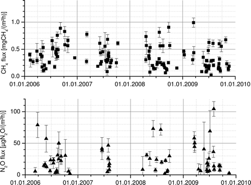
Figure 3. Observed mean annual night-time (22:00 h–06:00 h) fluxes for CH₄ (upper panel) and N₂O (lower panel) in black. The inventory-based flux estimates are given in dark gray. The data coverage for N₂O is too low for 2007 and is thus neglected. For CH₄ the light gray bars give the inventory-based flux estimates after adjusting the EDGARV4.1 inventory according to EC statistics. For N₂O the light gray bars include the seasonal cycle of agricultural N₂O emissions from IER (2009).

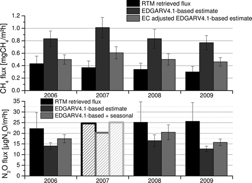
Although tempting, we restrain from discussing the observational flux to inventory-based flux difference on the annual time-scale or interpreting inter-annual changes of the observational fluxes, as these estimates strongly rely on the Radon emissions used. Using radon emissions from the Schery and Wasiolek (1998) map that does not account for inter-annual variability this could be causing some of the apparent changes as the inter-annual variability of the global radon flux is expected to be about 10% (Hirao et al. 2010). To interpret the year to year variation of the estimated RTM fluxes properly we would need yearly varying emission maps or continuous local flux observations of Radon; these will have to be included in future studies. We will thus focus our discussion only on the mean of our four-year period as this is a more robust result. The overall total of our measurement period is 0.36 ± 0.08 mgCH4/(m²h). This lies well below the inventory-based estimate of the mean for this time period, i.e. 0.79 ± 0.06 mgCH₄/(m²h). To further analyze the cause of this discrepancy we compare the footprint of situations when the inventory-based flux lies within the range of the observational estimate (0–1.07 mgCH₄/(m²h)) (Figure 4A) and the nights when the inventory-based estimate lies above it (Figure 4B). For the lower range data we find a rather symmetric area of influence and the inventory-based estimate of 0.53 ± 0.04 mgCH₄/(m²h) is closer to the observations of 0.36 ± 0.07 mgCH₄/(m²h) for this catchment area. For the situations when the inventory-based emissions are higher than the observational range, a stronger influence from the south-easterly sector is apparent. This area of influence comprises the GTA. Here, the inventory-based estimate is 1.65 ± 0.11 mgCH4/(m²h), thus significantly above the mean observational estimate of 0.37 ± 0.08 mgCH₄/(m²h) for the same region. Although there is some uncertainty in calculating the footprint it seems very unlikely that the transport model failed during all 29 individual nights belonging to this subset of our data. The discrepancy can rather be explained by an overestimation of the CH₄ fluxes from this region (Greater Toronto Area and the adjacent states of the U.S.) in the inventory. We also find a significant discrepancy when comparing the bottom-up flux estimates reported for Ontario by Environment Canada (EC 2010) and the EDGARV4.1 inventory (EDGAR 2010; see Table 1). The major differences are in the waste and energy sector, which are the main sources of CH₄ in the GTA, where the energy sector accounts for over 50% of the flux. Another indication pointing toward too large CH₄ fluxes in the EDGAR inventory is the observed ratio of CH₄ to N₂O fluxes. In the inventory we find that this ratio ranges from 20 to 200 mgCH₄/mgN₂O in rural areas and from 200 to over 500 mgCH₄/mgN₂O for the GTA while our observational estimates have a inter-quartiles range of 70–170 mgCH₄/mgN₂O. When adjusting the CH₄ fluxes in this footprint according to the EC inventory we see a decrease of the inventory-based flux estimate by about 60%, i.e. from 1.65 to 0.66 mgCH₄/(m²h), which lies considerably closer to our observations. Furthermore, the emission ratio of CH₄ to N₂O in the GTA drops to a very reasonable range of 100 to 300 mgCH₄/mgN₂O.

Figure 4. Contribution to the mean flux (logarithmic scale from 10⁰ (red) to 10⁻⁶ (blue)) for the nights when (A) the inventory-based flux predictions for CH₄ are within the range of the observational fluxes, (B) the inventory-based flux predictions for CH₄ are above the observed range, (C) the observational flux estimates for N₂O are within the range of the inventory predictions, (D) the observational data is above the range of N₂O fluxes predicted by the inventory. These maps were created with Google Earth ( http://earth.google.com).

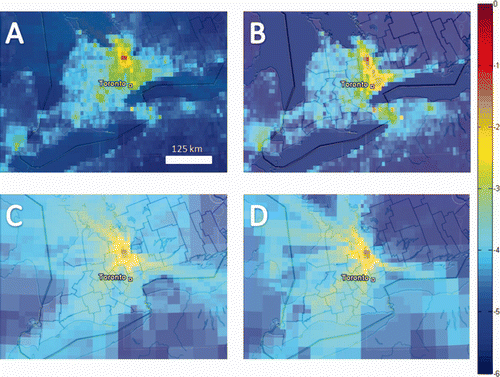
Table 1. CH₄ emissions in Ontario, Canada, from the official Environment Canada (EC 2010) and the EDGAR V41 inventory (EDGAR 2010). The categories are according to the EC nomenclature, with others comprising EDGAR categories that could not be allotted.

CH4 flux in Ontario [ktCH4/a]	Energy	Agriculture	Waste	Others	Total
EDGAR V4.1	470	247	572	19	1308
Environment Canada for 2005	120	210	320	–	650

3.3. N₂O fluxes in Southern Ontario derived from in-situ observations using the RTM

The data coverage for N₂O is unfortunately notably sparser and only includes 68 nights, (see Figure 2; lower panel). This is mostly, due to the bad signal-to-noise ratio of the N₂O measurements, which prevents the RTM algorithm from deriving meaningful fluxes. The observational flux estimates range from 7.6 to 31.2 μgN₂O/(m²h), for the inter-quartiles subset. Here, the inventory-based model predicts a inter-quartiles range of 8.7 to 19.0 μgN₂O/(m²h). We find that the mean annual observation-based flux estimates (see Figure 3; lower panel) are higher than any flux that can be derived from the EDGAR inventory. This was to be expected as the EDGARV4.1 inventory does not include non-anthropogenic N₂O sources. The overall mean for the N₂O fluxes is 24.4 ± 5.6 μgN₂O/(m²h) for our observations, while the inventory-based flux has a mean of 14.8 ± 1.0 μgN₂O/(m²h) for the same period of time. This translates to an underestimation of the N₂O fluxes by a factor of 1.65 ± 0.39 in the inventory. A campaign-based study of North America (Kort et al. 2008) found an underestimation by a factor of 2.62 ± 0.5 for the EDGAR3.2FT and a factor of 3.05 ± 0.61 for the GEIA inventory. They suggested that the underestimation was due to a lacking seasonal variation in the emission inventories. It is reasonable to assume that the N₂O release is not constant throughout the year but is linked to the agricultural activities involved in, e.g. growing crops. This could be an issue here as well, as (i) the catchment area includes significant agricultural areas to the south-west and (ii) the data coverage is better in summer where the emissions from agriculture are presumably higher. In a European high-resolution emission inventory for GHGs the agricultural emissions for the period from April to November are reported to lie 24% above the annual average (IER 2009), which would account for half of our deviation. When comparing the footprint belonging to the observational data above the range of the inventory-based estimates (Figure 4D) we find it not to be strikingly different from the rest of the dataset (Figure 4C). This indicates that this underestimation is not due to missing emissions in the adjacent urban area. Another contribution to the missing N₂O could be the missing natural fluxes in the inventory which are reported to be of the order of 10 μgN₂O/(m²h) for unfertilized soils in the U.S. (Mosier et al. 1991). A study of forests in Southern Ontario found a large range of N₂O fluxes from −52 to 24 μgN₂O/(m²h) for individual flux measurements with annual mean fluxes of up to 5.4 μgN₂O/(m²h) reported for 2007 (Peichl et al. 2010). To be able to better disjoin the mismatch of RTM retrieved fluxes and inventory-based estimates, future studies have to be performed when seasonally varying emission inventories for N₂O become available.

4. Summary and conclusions

We performed a pseudo-data experiment to demonstrate the capabilities and limitations of the RTM to assess currently available emission inventories. We found that when comparing the RTM results with simple bottom-up annual mean fluxes, biases of −4% for CH₄ and −25% for N₂O could arise. We therefore recommend that future studies using the RTM should include a high-resolution transport model to calculate footprints for the individual nights for comparison. If this precaution is take, the RTM can be used to retrieve the regional GHG fluxes and compare them with emission inventory data. In order to interpret inter-annual changes of the GHG fluxes the true flux of Radon has to be known, either from an accurate map or co-located Radon flux measurements in the catchment area.

Using the in-situ observations at the site in Egbert, Ontario we derived annual mean CH₄ fluxes from 2006 to 2009 ranging from 0.30 to 0.43 mgCH₄/(m²h) with a mean value of 0.36 ± 0.08 mgCH₄/(m²h). Our comparison of RTM derived CH₄ fluxes using in-situ measurements found a significant discrepancy to the flux predictions from the inventory. With the help of our Lagrangian model, we could identify that this is likely due to an overestimation of the CH₄ fluxes in the GTA. Here, the inventory-based estimate of 1.65 ± 0.11 mgCH₄/(m²h) is significantly above the observed mean of 0.37 ± 0.08 mgCH₄/(m²h).

The annual mean fluxes for N₂O ranged from 22.2 to 25.7 μgN₂O/(m²h) with a mean of 24.4 ± 5.6 μgN₂O/(m²h). Our findings that the observation-based fluxes of N₂O are above the inventory-based predictions by a factor of 1.7 ± 0.4 for our regions are in line with another study in North America (Kort et al. 2008). For our region this deviation could be explained by assuming seasonally varying emissions for N₂O and natural N₂O fluxes, neglected in the used emission inventory. Future investigations should allow separating the different influences when seasonally varying emission inventories for non-CO₂ GHGs become available.

The flux ratio of CH₄ to N₂O of the GTA in the model was well above the observed range, supporting the conclusion that the inventory emissions are underestimated. Using the reported bottom-up CH₄ emissions for Ontario from Environment Canada which deviate especially for the emissions in the energy and waste sector significantly reduced the difference between the inventory-based estimate and the observations. These results are promising for further applications of the RTM in the context of understanding urban GHG emissions.

Since modeling the emissions of GHGs of mega cities and large agglomerations is difficult for emission inventories (Dhakal 2010), the RTM approach could allow for an independent monitoring of urban areas which are expected to account for a significant share of the global anthropogenic emissions, e.g. 21–34% for CH₄, i.e. 7–15% of the global budget of CH₄ (Wunch et al. 2009). Our results indicate the in-situ sites used for the RTM should in general be close to the source to increase the signal-to-noise ratio.

The RTM has the potential of becoming a key tool to help improving the emission estimates for relevant tracers with high bottom-up uncertainties such as CH₄, N₂O, and other non-CO₂ GHGs on regional and continental scale. As more and more in-situ sites will become available in planned future regional and global monitoring networks, such as the Integrated Carbon Observation System (ICOS) ( http://www.icos-infrastructure.eu/) and the Earth Network ( http://www.earthnetworks.com/) the RTM could be applied at multiple sites that will have large parts of the highly populated regions of e.g. Europe in their catchment. To reduce the uncertainty of the RTM-based flux estimates a crucial step will be to reduce the uncertainties of the ²²²Radon flux, which currently is the limiting factor. This can be achieved by developing a parametrized ²²²Radon emission model, that accounts for short-term processes such as varying soil water levels and snow cover, which are still a problem for the currently available maps or, ideally, the ²²²Radon flux could also be monitored within these observational networks. Another important requirement to make best use of the RTM-base flux estimates is that these studies include high-resolution atmospheric modeling so one can distinguish different source regions within the catchment area and give a helpful feedback about the spatial distribution of the emissions to the bottom-up community.

Acknowledgements

The authors would like to thank Michele Ernst, Lauriant Giroux, Robert Kessler and Senen Racki for their diligent care and efforts for the GHG measurements of Environment Canada. We thank Ralf Staebler for his comments on our manuscript and we especially thank John C. Lin (University of Waterloo) for his support with the STILT modeling. This work was supported by the Environment Canada Clean Air Regulatory Agenda (CARA) and funding received by F.R.V. through a Visiting Fellowship to the Canadian Government Laboratories Award by the National Science and Engineering Research Council of Canada (NSERC). We furthermore want to thank the two anonymous reviewers for the thoughtful reviews that helped to improve the manuscript.

References

- Bergamaschi , P , Krol , M , Meirink , J F , Dentener , F , Segers , A , van Aardenne , J , Monni , S , Vermeulen , A T , Schmidt , M Ramonet , M . 2010 . Inverse modeling of European CH4 emissions 2001–2006 . J Geophys Res , 115 ( D22 ) : D22309
- Bousquet , P , Ciais , P , Miller , J B , Dlugokencky , E J , Hauglustaine , D A , Prigent , C , van der Werf , GR , Peylin , P , Brunke , E G Carouge , C . 2006 . Contribution of anthropogenic and natural sources to atmospheric methane variability . Nature , 443 ( 7110 ) : 439 – 443 .
- Corazza , M , Bergamaschi , P , Vermeulen , A T , Aalto , T , Haszpra , L , Meinhardt , F , O'Doherty , S , Thompson , R , Moncrieff , J Popa , E . 2011 . Inverse modelling of European N2O emissions: assimilating observations from different networks . Atmos Chem Phys , 11 ( 5 ) : 2381 – 2398 .
- Dhakal , S . 2011 . GHG emissions from urbanization and opportunities for urban carbon mitigation . Curr Opon Envirnm Sust , 2 ( 4 ) : 277 – 283 .
- [EC] Environment Canada, Government of Canada . 2010 . National Inventory Report 1990–2008: Greenhouse Gas Sources and Sinks in Canada [Internet] . The Canadian Government's Submission to the UN Framework Convention on Climate Change; [cited 2012 May 18] , Available from: http://www.ec.gc.ca/Publications
- [EDGAR] . Emission Database for Global Atmospheric Research release version 4.1 of the European Commission. 2010. Joint Research Centre (JRC)/Netherlands Environmental Assessment Agency (PBL) [Internet]; [cited 2012 May 18] Available from: http://edgar.jrc.ec.europa.eu
- Gerbig , C , Lin , J C , Wofsy , S C , Daube , B C , Andrews , A E , Stephens , B B , Bakwin , P S and Grainger , C A . 2003 . Toward constraining regional-scale fluxes of CO2 with atmospheric observations over a continent: 1. Observed spatial variability from airborne platforms . J Geophys Res-Atmos , 108 : 4756
- Griffiths , A D , Zahorowski , W , Element , A and Werczynski , S . 2010 . A map of radon flux at the Australian land surface . Atmos Chem Phys , 10 ( 18 ) : 8969 – 8982 .
- Hammer , S and Levin , I . 2009 . Seasonal variation of the molecular hydrogen uptake by soils inferred from continuous atmospheric observations in Heidelberg, southwest Germany . Tellus B , 61 ( 3 ) : 556 – 565 .
- Hirao , S , Yamazawa , H and Moriizumi , J . 2010 . Estimation of the global 222Rn flux density from the Earth's surface . Jpn J Health Phys , 45 ( 2 ) : 161 – 171 .
- [IER] Institut für Energiewirtschaft und Rationelle Energieanwendung . 2009 . Spatial and temporal disaggregation of anthropogenic greenhouse gas emissions in Europe: Emission Inventory for Europe 2005 Available from: http://carboeurope.ier.uni-stuttgart.de/
- [IPCC] Intergovernmental Panel on Climate Change . 2007 . “ Climate change 2007: the physical science basis ” . In Contribution of working group I to the fourth assessment report of the Intergovernmental Panel on Climate Change , Edited by: Solomon , S , Qin , D , Manning , M , Chen , Z , Marquis , M , Averyt , K B , Tignor , M and Miller , H L . 131 – 144 . Cambridge (UK) and New York (NY) : Cambridge University Press .
- Jonas , M , White , T , Marland , G , Lieberman , D , Nahorski , Z and Nilsson , S . 2010 . Coping with uncertainty. Berlin (Heidelberg): Springer . Chapter 11, Dealing with uncertainty in GHG inventories: how to go about it? , : 229 – 245 .
- Kort , E A , Eluszkiewicz , J , Stephens , B B , Miller , J B , Gerbig , C , Nehrkorn , T , Daube , B C , Kaplan , J O , Houweling , S and Wofsy , S C . 2008 . Emissions of CH4 and N2O over the United States and Canada based on a receptor-oriented modeling framework and COBRA-NA atmospheric observations . Geophys Res Lett , 35 ( 18 ) : L18808
- Krystek , M and Anton , M . 2007 . A weighted total least-squares algorithm for fitting a straight line . Meas Sci Technol , 18 ( 11 ) : 3438 – 3442 .
- Levin , I , Born , M , Cuntz , M , Langendörfer , U , Mantsch , S , Naegler , T , Schmidt , M , Varlagin , A , Verclas , S D and Wagenbach , D . 2002 . Observations of atmospheric variability and soil exhalation rate of radon-222 at a Russian forest site . Technical approach and deployment for boundary layer studies. Tellus B , 54 : 462 – 475 .
- Levin , I , Glatzel-Mattheier , H , Marik , T , Cuntz , M , Schmidt , M and Worthy , D EJ . 1999 . Verification of German methane emission inventories and their recent changes based on atmospheric observations . J Geophys Res , 104 : 3447 – 3456 .
- Levin , I , Hammer , S , Eichelmann , E and Vogel , F R . 2011 . Verification of greenhouse gas emission reductions: the prospect of atmospheric monitoring in polluted areas . Phil Trans R Soc A , 369 ( 1943 ) : 1906 – 1924 .
- Lin , J C , Gerbig , C , Wofsy , S C , Andrews , A E , Daube , B C , Davis , K J and Grainger , C A . 2003 . A near-field tool for simulating the upstream influence of atmospheric observations: the Stochastic Time-Inverted Lagrangian Transport (STILT) model . J Geophys Res , 108 ( D16 ) : 4493
- Manning , A J , Ryall , D B , Derwent , R G , Simmonds , P G and O'Doherty , S . 2003 . Estimating European emissions of ozone-depleting and greenhouse gases using observations and a modeling back-attribution technique . J Geophys Res-Atmos , 108 ( D14 ) : ACH3-1
- Messager , C , Schmidt , M , Ramonet , M , Bousquet , P , Simmonds , P , Manning , A , Kazan , V , Spain , G , Jennings , S G and Ciais , P . 2008 . Ten years of CO2, CH4, CO and N2O fluxes over Western Europe inferred from atmospheric measurements at Mace Head, Ireland . Atmos Chem Phys Discuss , 8 ( 1 ) : 1191 – 1237 .
- Mosier , A , Schimel , D , Valentine , D , Bronson , K and Parton , W . 1991 . Methane and nitrous oxide fluxes in native, fertilized and cultivated grasslands . Nature , 350 ( 6316 ) : 330 – 332 .
- Montzka , S A , Dlugokencky , E J and Butler , J H . 2011 . Non-CO2 greenhouse gases and climate change . Nature , 476 ( 10322 ) : 43 – 50 .
- Nisbet , E and Weiss , R . 2010 . Top-down versus bottom-up . Science , 328 ( 5983 ) : 1241 – 1243 .
- [NRC] Committee on Methods for Estimating Greenhouse Gas Emissions of the National Research Council . 2010 . Verifying greenhouse gas emissions , Washington , DC : The National Academic Press .
- Olivier , J GJ , Bouwman , A F , Berdowski , J JM , Veldt , C , Bloos , J PJ , Visschedijk , A JH , van der Maas , CWM and Zandveld , P YJ . 1999 . Sectoral emission inventories of greenhouse gases for 1990 on a per country basis as well as on 1° × 1° . Environ Sci Pol , 2 ( 3 ) : 241 – 263 .
- Peichl , M , Arain , M A , Ullah , S and Moore , T R . 2010 . Carbon dioxide, methane, and nitrous oxide exchanges in an age-sequence of temperate pine forests . Glob Change Biol , 16 : 2198 – 2212 .
- Peylin , P , Houweling , S , Krol , M C , Karstens , U , Rödenbeck , C , Geels , C , Vermeulen , A , Badawy , B , Aulagnier , C Pregger , T . 2011 . Importance of fossil fuel emission uncertainties over Europe for CO2 modeling: model intercomparison . Atmos Chem Phys , 11 ( 13 ) : 6607 – 6622 .
- Pison , I , Bousquet , P , Chevallier , F , Szopa , S and Hauglustaine , D . 2009 . Multi-species inversion of CH4, CO and H2 emissions from surface measurements . Atmos Chem Phys , 9 ( 14 ) : 5281 – 5297 .
- Ryall , D B , Derwent , R G , Manning , A J , Simmonds , P G and O'Doherty , S . 2001 . Estimating source regions of European emissions of trace gases from observations at Mace Head . Atmos Environ , 35 ( 14 ) : 2507 – 2523 .
- Schery , S D and Wasiolek , M A . 1998 . “ Radon and Thoron in the human environment ” . In Modeling Radon flux from the earth's surface , Edited by: Akira K, Michikuni , S . 207 – 217 . Singapore : World Scientific Publishing .
- Schmidt , M , Glatzel-Mattheier , H , Sartorius , H , Worthy , D EJ and Levin , I . 2001 . Western European N2O emissions: a top-down approach based on atmospheric observations . J Geophys Res , 106 : 5507 – 5516 .
- [StatsCan] , Statistics Canada and Govermnent , of Canada . 2008 . Census 2006 [Internet]; [cited 2011 October 4] Available from: http://www40.statcan.gc.ca/
- Szegvary , T , Conen , F and Ciais , P . 2009 . European 222Rn inventory for applied atmospheric studies . Atmos Environ , 43 : 1536 – 1539 .
- Szegvary , T , Leuenberger , M C and Conen , F . 2007 . Predicting terrestrial 222Rn flux using gamma dose rate as a proxy . Atmos Chem Phys , : 2789 – 2795 .
- Worthy , D EJ . 2003 . Canadian baseline program: summer of progress to 2002 Canada , , Environment Canada, Meteorological Service of Canada
- Wunch , D , Wennberg , P O , Toon , G C , Keppel-Aleks , G and Yavin , Y G . 2009 . Emissions of greenhouse gases from a North American megacity . Geophys Res Lett , 36 : L1581
- Zhang , K , Feichter , J , Kazil , J , Wan , H , Zhuo , W , Griffiths , A D , Sartorius , H , Zahorowski , W , Ramonet , M Schmidt , M . 2011 . Radon activity in the lower troposphere and its impact on ionization rate: a global estimate using different radon emissions . Atmos Chem Phys , 11 ( 15 ) : 7817 – 7838 .