Greenhouse gas emissions and mitigation potentials in agriculture, forestry and other land use in Southeast Asia

Abstract

This study aims to estimate greenhouse gas (GHG) emissions and mitigation potentials in Agriculture, Forestry and Other Land Use (AFOLU) in the Southeast Asian countries: Indonesia, Malaysia and Vietnam, up to 2030. We developed a bottom-up type model named the AFOLUB Model, which calculates GHG mitigations based on the detailed information of specific technologies. The model illustrates producer's behaviour of agricultural production and mitigation technology selection as a result of profit maximization. Using this model, we evaluated mitigations and effective technologies with high mitigation potentials in the sectors. As a result, GHG emissions in agriculture and Land Use, Land-Use Change and Forestry (LULUCF) in the three countries were 149 MtCO₂eq/year and 1.0 GtCO₂eq/year in 2005 and will increase 1.7 and 1.8 times up to 2030 in the BaU case. Indonesia is the largest emission country among them. We also found that no-regret mitigation technologies are expected to reduce 33MtCO₂eq/year in 2030, which corresponds to 22% of agricultural emissions at the 2005 level. Under 10USD/tCO₂eq of mitigation cost, 56MtCO₂eq/year of emissions can be reduced by midseason drainage (MM) in rice cultivation, high efficient fertilizer application (HEF) to managed soils and Replacement of roughage with concentrates (RRC) etc.

Keywords:

• climate change
• agriculture
• land-use change
• mitigation potentials
• Southeast Asia

Introduction

To achieve the target of cutting global greenhouse gas (GHG) emissions in half by 2050, governments have started assessing mitigation strategies for reducing their domestic GHG emissions.

The Agriculture, Forestry and Other Land Use (AFOLU) sector, contribute 31% of the global anthropogenic GHG emissions in 2004 (IPCC, 2007). In Indonesia, Malaysia and Vietnam, the AFOLU sector constitutes 67%, 16% and 53% of the domestic emissions in 2000 (MoE 2010; MONRE 2010; NRE 2011). The governments have estimated domestic GHG mitigation potentials across multiple sectors. Especially for Indonesia, TNA (MoE 2009); DNPI (2010); Rizaldi (2001) have dealt comprehensively with many types of mitigation technologies, and they estimated mitigation potentials for each technology. However, they assumed amounts of technologies to be applied in the future based on expert judgement. They did not answer to a question how much amounts of which mitigation technologies are applied to reduce GHG emission the most economic efficiently.

In this study, we developed a model named the AFOLU Bottom-up Model for GHG emission mitigation (AFOLUB Model) and applied the model to the three countries. Using the model, we analyzed quantitatively mitigation potentials up to 2030 and amounts of GHG mitigation technologies to be applied in the future. We also proposed mitigation technologies, which have a high economic efficiency, in the AFOLU sector.

AFOLUB model

Basic concept of AFOLUB model

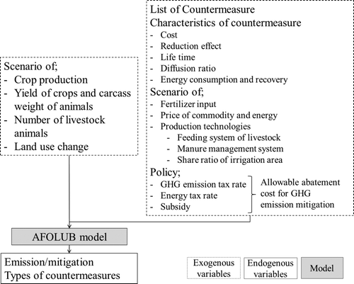
The AFOLUB model is a bottom-up type model to estimate GHG emissions, mitigation potentials in the AFOLU sector at the national/regional level, based on detailed information of specific technologies. The model illustrates amounts and combinations of the technologies to be applied by agricultural producers (i.e. farmers) under economic rationality. The amounts and combinations are calculated so as to ensure the assumption that producers select the technologies appropriately in order to maximize their annual profits. In the model, future assumptions of agricultural production and land use change are given exogenously. Based on the assumptions, the AFOLUB model solves the profit maximization problem.

Input and output of AFOLUB model

Figure 1 shows input and output of AFOLUB model. Input to the AFOLUB model is as: (1) list of climate change mitigation technologies; (2) characteristics of each technology; (3) future assumptions on production and productivity of agricultural commodities and land-use change; (4) future assumptions of commodity prices; (5) production technologies, manure management systems and their economic characteristics and finally; (6) Allowable Abatement Cost (AAC) for GHG emission mitigation. The AAC is a representative parameter for incentive or disincentive for GHG mitigations i.e. an emission tax rate and a ratio of subsidy.

Figure 1. Input and output of AFOLUB model.

Cost

The model concerns only extra cost which is caused by installation of mitigation technologies. The extra cost is defined to be a difference from a cost in the base year. Costs taken up in the model include (1) additional wage for mitigation technologies; (2) additional initial and O&M cost and (3) AAC, producer subsidy, production tax. Cost and benefit for land conversion is not taken into account.

Emission sources

We followed the IPCC Inventory Guidelines (GL2006, 2006) for classification of GHG emission sources. Table 1 shows the GHG emission sources, agricultural commodities, types of GHGs treated in the AFOLUB model and emission categories defined in the IPCCGL (1996 and 2006).

Table 1. Greenhouse gas emission sources covered in AFOLUB model and the categories of IPCC guideline.

Emission sources	Classification	Gases	IPCC GLs 2006	IPCC GLs 1996
Enteric fermentation		CH4	3A1	4A
	Dairy cattle		3A1ai	4A1a
	Other cattle		3A1aii	4A1b
	Buffalo		3A1b	4A2
	Sheep		3A1c	4A3
	Goats		3A1d	4A4
	Camels		3A1e	4A5
	Horses		3A1f	4A6
	Mules		3A1g	4A7
	Asses		3A1g	4A7
	Swine		3A1h	4A8
Manure management		CH4, N2O	3A2	4B
	Dairy cattle		3A2ai	4B1a
	Other cattle		3A2aii	4B1b
	Buffalo		3A2b	4B2
	Sheep		3A2c	4B3
	Goat		3A2d	4B4
	Camel		3A2e	4B5
	Horse		3A2f	4B6
	Mules		3A2g	4B7
	Asses		3A2g	4B7
	Swine		3A2h	4B8
	Chickens		3A2i	4B9
	Ducks		3A2i	4B9
	Turkeys		3A2i	4B9
Landuse, Landuse change and Forestry (LULUCF)		CO2	3B	5
	Forest land		3B1	5A, 5B, 5D
	Cropland		3B2	4C, 4D, 4F, 5A, 5B, 5D
	Grassland		3B3	4D, 4E, 5A, 5B, 5C, 5D
	Wetlands		3B4	5A, 5B, 5E, 4D
	Settlements		3B5	5A, 5D, 5E, 5B
	Other land		3B6	–
Aggregate sources and non-CO2 emissions sources on land			3C	–
	Emissions from biomass burning*	CO2, CH4, N2O	3C1	–
	Liming*	CO2	3C2	–
	Urea application*	CO2	3C3	–
	Direct N2O emission from managed soils	N2O	3C4	4D
	Indirect N2O emission from managed soils	N2O	3C5	4D
	Indirect N2O emissions from manure management	N2O	3C6	–
Rice cultivations		CH4	3C7	4C
Note: *Not estimated by AFOLUB model.

Table 2. List of main technology (l0).

Code	Main technologies (l0)	Code	Main technologies (l0)
Livestock enteric fermentation		Manure management
gz_cattle_d	Grazing dairy cattle	lmc_cattle_d	Manure management for dairy cattle
gz_cattle_o	Grazing other cattle	lmc_cattle_o	Manure management for other cattle
gz_buffaloes	Grazing buffalo	lmc_buffaloes	Manure management for buffalo
gz_sheep	Grazing sheep	lmc_sheep	Manure management for sheep
gz_goats	Grazing goats	lmc_goats	Manure management for goats
gz_camels	Grazing camels	lmc_camels	Manure management for camels
gz_horses	Grazing horses	lmc_horses	Manure management for horses
gz_mules	Grazing mules	lmc_mules	Manure management for mules
gz_asses	Grazing asses	lmc_asses	Manure management for asses
gz_swines	Grazing swines	lmc_swines	Manure management for swines
ho_cattle_d	Housing dairy cattle	lmc_chickens	Manure management for chickens
ho_cattle_o	Housing other cattle	lmc_ducks	Manure management for ducks
ho_buffaloes	Housing buffalo	lmc_turkeys	Manure management for turkeys
ho_sheep	Housing sheep	Managed soils
ho_goats	Housing goats	n_pdr	Nitogen fertilizer application to rice field
ho_camels	Housing camels	n_wht	Nitogen fertilizer application to wheat field
ho_horses	Housing horses	n_gro	Nitogen fertilizer application to other coarse grains field
ho_mules	Housing mules	n_v_f	Nitogen fertilizer application to vegetable, fuites and nuts field
ho_asses	Housing asses	n_osd	Nitogen fertilizer application to oil crops field
ho_swines	Housing swines	n_c_b	Nitogen fertilizer application to sugar crops field
ho_chickens	Housing chickens	n_ocr	Nitogen fertilizer application to other crops field
ho_ducks	Housing ducks	navb_cattle_d	Application of manure compost of dairy cattle to managed soils
ho_turkeys	Housing turkeys	navb_cattle_o	Application of manure compost of other cattle to managed soils
Manure management		navb_buffaloes	Application of manure compost of buffalo to managed soils
ms1	Uncovered anaerobic lagoon	navb_sheep	Application of manure compost of sheep to managed soils
ms2	Liquid/Sherry	navb_goats	Application of manure compost of goats to managed soils
ms3	Solid storage	navb_camels	Application of manure compost of camels to managed soils
ms4	Drylot	navb_horses	Application of manure compost of horses to managed soils
ms5	PRP	navb_mules	Application of manure compost of mules to managed soils
ms6	Daily spread	navb_asses	Application of manure compost of asses to managed soils
ms7	Digester	navb_swines	Application of manure compost of swines to managed soils
ms8	Burned for fuel or as waste	navb_chickens	Application of manure compost of chickens to managed soils
ms9	Pit<1 month	navb_ducks	Application of manure compost of ducks to managed soils
ms10	Pit>1 month	navb_turkeys	Application of manure compost of turkeys to managed soils
ms11	Other	Rice cultivation
ms12	Anaerobic digester	pdy	Rice production in flooded field
ms13	Cattle and swine deep bedding	dpdy	Rice production in upland field
ms14	Composting – In-vessel
ms15	Composting – Static pile
ms16	Composting – Intensive windrow
ms17	Composting – Passive windrow
ms18	Poultry manure with litter
ms19	Poultry manure without litter
ms20	Aerobic treatment

Table 3. List of additional technologies in agriculture (l1∼lN).

Emission source	Code	Additional technology (l1∼lN)		References	Mitigation [tCO2eq/ha/year] or [tCO2eq/head/year]	Reference country
Livestock enteric fermentation	3A1	HGM	High genetic merit	Bates (1998)	0.32	XE15
		RRC	Replacement of roughage with concentrates	Bates (1998), Shibata and Fujimori (2010), Graus et al. (2004)	0.45	XE15
		DSM	Daily spread of manure	Bates (1998)	0.33	XE15
Manure management	3A2	CFL	Biogas capture	USEPA (2006), MoE (2010) pp.V-30, NRE (2011) p. 33 Table 3.1, MONRE (2010) p. 100.	0.62	USA
Managed soils	3C4-3C6	HEF	High efficienct fertilizer application	USEPA (2006), Hendriks et al. (1998), Amann et al. (2008)	0.65	USA
		TRM	Tillage and residue management	IPCC (2007), Smith et al. (2007)	0.08	XE15
		SRF	Use of slow-release type fertilizers, polymer-coated fertilizers	USEPA (2006), Akiyama et al. (2010)	0.76	USA
Rice cultivation	3C7	RAS	Replace urea with ammonium sulfate	USEPA (2006), Graus et al. (2004) p. 16	0.24	USA
		MD	Midseason drainage	USEPA (2006), NRE (2011), p. 33, Table 3.1, MONRE (2010) p. 100	0.89	USA
		FIR	Fall incorporation of rice straw	USEPA (2006)	0.68	USA

Table 4. List of main activity (jd).

Code	Main activitiy (jd)	Index	Unit of index
pdr	Rice production	Harvested area	ha
dpdr	Rice production	Harvested area	ha
wht	Wheat production	Harvested area	ha
gro	Other coarse grain production	Harvested area	ha
v_f	Vegetable, fuites and nut production	Harvested area	ha
osd	Oil crop production	Harvested area	ha
c_b	Sugar crop production	Harvested area	ha
ocr	Other crop production	Harvested area	ha
gz_cattle_d	Milk production by grazing	Number of grazing animals	head
gz_cattle_o	Beef production by grazing	Number of grazing animals	head
gz_buffaloes	Buffalo meat production by grazing	Number of grazing animals	head
gz_sheep	Sheep meat production by grazing	Number of grazing animals	head
gz_goats	Goat meat production by grazing	Number of grazing animals	head
gz_camels	Camel meat production by grazing	Number of grazing animals	head
gz_horses	Horse meat production by grazing	Number of grazing animals	head
gz_mules	Mule meat production by grazing	Number of grazing animals	head
gz_asses	Asses meat production by grazing	Number of grazing animals	head
gz_swines	Pork production by grazing	Number of grazing animals	head
fd_cattle_d	Milk production by housing	Number of housing animals	head
fd_cattle_o	Beef production by housing	Number of housing animals	head
fd_buffaloes	Buffalo meat production by housing	Number of housing animals	head
fd_sheep	Sheep meat production by housing	Number of housing animals	head
fd_goats	Goat meat production by housing	Number of housing animals	head
fd_camels	Camel meat production by housing	Number of housing animals	head
fd_horses	Horse meat production by housing	Number of housing animals	head
fd_mules	Mule meat production by housing	Number of housing animals	head
fd_asses	Asses meat production by housing	Number of housing animals	head
fd_swines	Pork production by housing	Number of housing animals	head
fd_chickens	Chicken meat production by housing	Number of housing animals	head
fd_ducks	Duck meat production by housing	Number of housing animals	head
fd_turkeys	Turkey meat production by housing	Number of housing animals	head

Table 5. List of secondary activity (js).

Code	Secondary activitiy (js)	Index	Unit of index
n_pdr	Nitorus fertilizer application into rice paddy field	Harvested area	ha
ms1	Manure management by Uncovered anaerobic lagoon	Nitrogen in manure	ton N
ms2	Manure management by Liquid/Sherry	Nitrogen in manure	ton N
ms3	Manure management by Solid storage	Nitrogen in manure	ton N
ms4	Manure management by Drylot	Nitrogen in manure	ton N
ms5	Manure management by PRP	Nitrogen in manure	ton N
ms6	Manure management by Daily spread	Nitrogen in manure	ton N
ms7	Manure management by Digester	Nitrogen in manure	ton N
ms8	Manure management by Burned for fuel or as waste	Nitrogen in manure	ton N
ms9	Manure management by Pit<1 month	Nitrogen in manure	ton N
ms10	Manure management by Pit>1 month	Nitrogen in manure	ton N
ms11	Manure management by Other	Nitrogen in manure	ton N
ms12	Manure management by Anaerobic digester	Nitrogen in manure	ton N
ms13	Manure management by Cattle and swine deep bedding	Nitrogen in manure	ton N
ms14	Manure management by Composting – In-Vessel	Nitrogen in manure	ton N
ms15	Manure management by Composting – Static Pile	Nitrogen in manure	ton N
ms16	Manure management by Composting – Intensive Windrow	Nitrogen in manure	ton N
ms17	Manure management by Composting – Passive Windrow	Nitrogen in manure	ton N
ms18	Manure management by Poultry manure with litter	Nitrogen in manure	ton N
ms19	Manure management by Poultry manure without litter	Nitrogen in manure	ton N
ms20	Manure management by Aerobic treatment	Nitrogen in manure	ton N
lmc_cattle_d	Manure management for dairy cattle	Number of animals	head
lmc_cattle_o	Manure management for other cattle	Number of animals	head
lmc_buffaloes	Manure management for buffaloes	Number of animals	head
lmc_sheep	Manure management for sheep	Number of animals	head
lmc_goats	Manure management for goats	Number of animals	head
lmc_camels	Manure management for camels	Number of animals	head
lmc_horses	Manure management for horses	Number of animals	head
lmc_mules	Manure management for mules	Number of animals	head
lmc_asses	Manure management for asses	Number of animals	head
lmc_swines	Manure management for swines	Number of animals	head
lmc_chickens	Manure management for chickens	Number of animals	head
lmc_ducks	Manure management for ducks	Number of animals	head
lmc_turkeys	Manure management for turkeys	Number of animals	head
navb_cattle_d	Application of manure compost of dairy cattle to managed soils	Nitrogen in manure applied to soils	ton N
navb_cattle_o	Application of manure compost of other cattle to managed soils	Nitrogen in manure applied to soils	ton N
navb_buffaloes	Application of manure compost of buffaloes to managed soils	Nitrogen in manure applied to soils	ton N
navb_sheep	Application of manure compost of sheep to managed soils	Nitrogen in manure applied to soils	ton N
navb_goats	Application of manure compost of goats to managed soils	Nitrogen in manure applied to soils	ton N
navb_camels	Application of manure compost of camels to managed soils	Nitrogen in manure applied to soils	ton N
navb_horses	Application of manure compost of horses to managed soils	Nitrogen in manure applied to soils	ton N
navb_mules	Application of manure compost of mules to managed soils	Nitrogen in manure applied to soils	ton N
navb_asses	Application of manure compost of asses to managed soils	Nitrogen in manure applied to soils	ton N
navb_swines	Application of manure compost of swines to managed soils	Nitrogen in manure applied to soils	ton N
navb_chickens	Application of manure compost of chickens to managed soils	Nitrogen in manure applied to soils	ton N
navb_ducks	Application of manure compost of ducks to managed soils	Nitrogen in manure applied to soils	ton N
navb_turkeys	Application of manure compost of turkeys to managed soils	Nitrogen in manure applied to soils	ton N

Ruminant animals cause CH₄ emissions by enteric fermentation (3A1) Manure of livestock animals cause CH₄ emission due to anaerobic conditions (3A2). In a process of manure management, manure cause N₂O emission (3A2). Some manure is applied on pasture, range and paddock or on croplands as organic fertilizer. N₂O emissions from nitrogen included in the manure are classified as emission from managed soils (3C4 to 3C6). Rice is cultivated in wetland and upland fields. CH₄ emission comes only from wetland rice fields, and N₂O emission comes from nitrogen fertilizer of both rice fields. Greenhouse gas emissions from peat fire and harvested wood products in LULUCF sector are not taken into account.

Emission factors

We refer to tier 1 or 2 of the IPCC (2006) for the methodology to estimate GHG emissions. According to the guideline, GHG emissions are calculated as a product of activity and at least one factor. We calculated the emission factor by multiplying the factors.

Description of combinations of technologies

To capture both behaviours of producers: production and mitigation technology selection, the AFOLUB model concerns two types of technologies: agricultural production technologies and GHG mitigation technologies. In this study, the agricultural production technologies represent producer's activities to produce agricultural commodities (i.e. crop cultivation and grazing livestock animals). In the model, these two types of technologies are handled as one technology represented by a suffix l. For more general description, technology l is defined as a combination of;

1.	Main technology (l0): a technology to achieve main objective of human activities (i.e. Grazing dairy cattle (code: gz_cattle_d) is a main technology for milk production.).
2.	Additional technology (l1∼lN, N: the number of additional technologies combined to one main technology.): a technology to be added to the main technology for GHG mitigation. (i.e. High genetic merit (code: HGM) is a GHG mitigation technology for grazing dairy cattle (code: gz_cattle_d))

Tables 2 and 3 list the main technologies and additional technologies for agriculture sector respectively. Manure management systems excluding PRP defined as main technologies are applied only to housing animal, not to grazing animals since it is difficult to control manure of grazing animals. Only the PRP is applied to grazing animals.

Description of characteristics of technology changed by additional technology

Six characteristics of a technology: productivity (y_l ), cost (f_l ), emission factor (), maximum diffusion ratio (θmax_l ) and minimum diffusion ratio (θmin_l ) can be changed depending on additional technologies. To concern the changes, parameters of the six characteristics are adjusted by parameters of additional technologies represented by suffix LS as an equation (EQ_ADJY). The characteristics of the main technologies are represented by suffix l0. For example, to adjust a parameter of productivity y_l , productivity of main technology y_l0 is adjusted by ay_LS . The adjustments are used for decrease in crop productivity by reduced fertilizer and increase in livestock productivity by improved feed management etc. For emission factor (), synergetic effects by combining several mitigation technologies are considered by the same formula. In the following equation, δ _{l,l0,l1,…,lN} is a matrix to represent a possible/impossible combination of technologies; If technology combination (l = (l0,l1,…,lN)) is taken into account, δ _{l,l0,l1,…,lN} is 1, otherwise 0. We also concern a main technology without any additional technologies, which is represented by l0∼lN = dummy and ay_LS  = 1 for the dummy.

Structure of AFOLUB model

Greenhouse gas emission (Q_l ^m ) is calculated as a product of the amounts of technology l (X_l ) and an emission factor of a technology l (e_l ^m ) (EQ_EMISS).

Profit of producers is calculated from total sales of agricultural commodities, production costs and mitigation costs, and revenue from electricity generation or heat generation from recovering CH4 gases (EQ_PRF and EQ_COST).

It is assumed that more than one main technology (l) can be applied to one activity (j). A relation between technology (l) and activity (j) are described using a flag function δLJ_l,j . If l and j have a relation, δLJ_l,j is 1, otherwise 0. Amounts of technologies (X_l ) are counted by units of harvested areas of crops and numbers of livestock animals.

Cost includes wage, initial and O & M cost and AAC for GHG mitigation etc. (EQ_COST).

To capture systematically relations between amounts of activities in the model (i.e. amount of livestock's manure is calculated from number of animals.), there are two types of activities: main activity (jd) and secondary activity (js).

The main activity represents production of the commodity/service and the secondary activity represents activity caused by secondary products of agricultural production technologies. For example, meat production is a main activity for producers, and since manure is a secondary product of the meat production, manure management is a secondary activity. Tables 4 and 5 list main and secondary activities.

Production of commodity/service of main activity is given exogenously as DEX_jd . It is assumed that the commodities/services are produced by technology (l) and the production is calculated as a product of productivity (y_l ) and amount of technology (X_l ) (EQ_SPLY and EQ_DMD). The productivity represents a production per a unit of main technology, namely, crop production per a unit area or meat/milk production per animal. A relation of amounts between main and secondary activities is formulated with EQ_SEC(js). a_js,l is a factor to calculate amounts of secondary activity from amount of technology l. a_js,l is also calculated using IPCCGL(2006) methodology. Technology (l) is also conducted to the secondary activities (EQ_SPLY).

Maximum and minimum diffusion ratios of technology (θmax_l and θmin_l ) are assumed by equations (EQ_MIN) and (EQ_MAX). The ratios are a value from 0 to 1 and the unit of the ratio is a percentage to total amount of activity (D_j ).

Under these conditions (EQ_SPLY), (EQ_SEC), (EQ_DMD), (EQ_MIN) and (EQ_MAX), combination of technologies is calculated in order to maximize their profits (EQ_TPRF).

Notations

Unit of activity is represented in Table 1. An upper bar represents an exogenous variable.

j : Activity to produce commodity/service

jd : Main activity, jd(∈JD(J))

js : Secondary activity, js(∈Js(J))

l : Technology

LS: Group of additional technologies

m : Gas

Ljs : Group of technologies to produces secondary activity js[-]

: GHG emission [MtCO₂ eq/year]

X_l : Amount of technology l [activity/year]

D_j : Amount of commodity/service produced by activity j [ton/year]

Y_j : Profit from activity j [USD/year]

Φ : Total profit [USD/year]

y_l : Productivity of technology l [ton/activity]

p_j : Price of commodity/service produced by activity j [USD/ton]

f_l : Initial and O&M cost of technology l [USD/activity/year]

c_l : Cost of technology l [USD/activity/year]

: Allowable abatement cost for mitigation of gas m using technology l [USD/MtCO₂eq]

: Emission factor of gas m by operating a unit technology l [MtCO₂eq/activity/year]

a _js,l : Factor to calculate amount of secondary activity js from amouns of technology l[-]

θmin_l : Maximum diffusion ratio of technology l[-]

θmax_l : Matrix of a relation between technology l and activity j[-]

ayLS : Adjustment coefficients of parameter y_l [-]

Application of AFOLUB model to Southeast Asian countries

Framework of application

We estimated GHG emissions and mitigation potentials in the AFOLU sector from 2000 to 2030 as a one-year step in Southeast Asian countries, namely, Indonesia, Malaysia and Vietnam. Allowable Abatement Costs () are assumed as 0 to more than 100 USD/tCO₂eq. We assumed two scenarios: a case where no mitigation technologies are applied (BaU case), and a case where mitigation technologies are applied under the assumed AACs (CM case). Greenhouse gas mitigation potential is defined as a difference of GHG emissions between the two scenarios.

Future assumptions of activities and used data

As inputs to the AFOLUB, we developed future assumptions of harvested area of crops, number of livestock animals and area of land use change used in the discussion on climate mitigation in the AFOLU sectors. In developing the assumptions, in order to consider the country-specific situations and conditions, we referred to national statistics and governmental plans and projections (MoF 2008; BAPPENAS 2009; MoE 2010; MONRE 2010; NRE 2011; Wicke et al. 2011) wherever they were available. If the country-specific information was not available we used international statistics (IFA/FAO/IFDC, 1999, 2002; IRRI 2011; FAO 2012) for the base year. For the future, we extrapolated the harvested area and the animal numbers up to 2030 using a growth rate derived from the historical trend.

For area of land-use change, we assumed that country area and area of land and inland water are constant at the 2009 level and that forest area will change at a ratio shown in the government plans (MoE 2010; MONRE 2010; NRE 2011). Settlement is extrapolated up to 2030 using a population growth ratio (UN 2007). Cropland is extrapolated using a growth ratio of harvested area of crops. We assumed that area of reduced forestland is allocated into land categories where lands are increasing in the future (i.e. settlements). The rest of the deforested area is allocated into other land. For peat land, we assumed that 15,000 ha of peat land is annually drained for conversion into cropland in Indonesia.

We assumed that in the future, nitrogen fertilizer consumption will increase in proportion to yields. Crop price is sourced from data estimated and interpolated by Hasegawa (2009) using FAO (2007).

Assumptions of mitigation technology

We collected information on mitigation technologies from various international and domestic literatures (Bates 1998; Hendriks et al. 1998; Rizaldi 2001; Graus et al. 2004; USEPA 2005; USEPA 2006; Smith et al. 2007; Amann et al. 2008; Akiyama et al. 2010; Shibata and Fujimori 2010) and developed a database of technologies, which includes types of technologies, mitigation potential, costs and application terms etc. The reference cost is exchanged into costs in each country from reference country using wage, energy price and capital coat (World Bank 2006; Davis Langdon & Seah International 2010). Table 6 shows mitigation potentials of each technology in agriculture.

Results and discussions

GHG emissions in BaU case in AFOLU sectors

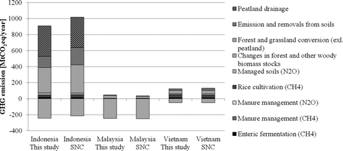
Figure 2 shows GHG emissions in 2000 in the AFOLU sectors compared to the Second National Communication to the UNFCCC (hereafter SNC) (MoE 2010; MONRE 2010; NRE 2011). Our results are similar to the SNC estimates.

Figure 2. Greenhouse gas emissions in Agriculture and LULUCF in 2000 comparing to SNC.

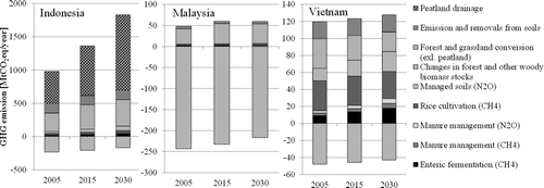
Figure 3 shows GHG emissions in the BaU case by 2030 in the AFOLU sectors. Different situations can be seen among the three countries. Indonesia is the largest emission country among them. In the country, total GHG emission in 2005 is 750 MtCO₂eq/year. Agricultural emission is 78MtCO₂eq/year and LULUCF emission and sink are 900 MtCO₂eq/year and –230 MtCO₂eq/year respectively. Land Use, Land-Use Change and Forestry emissions arise from peat land drainage (54%), followed by forest and grassland conversion (excluding peat land) (31%) and net emission from soils (15%). In 2030, total GHG emissions are increasing up to 1.5GtCO₂eq/year. Agriculture and LULUCF emission is increasing 2.1 times and 2.3 times from 2005 to 2030. In 2030, 67% of the LULUCF emissions derive from peat land drainage. The rest of the emission is increasing and the sink is decreasing due to the reduced forestland by 2030. In agriculture, there is a drastic increase in N₂O emissions from livestock (3A1 and 3A2) and managed soils (3C4 to 3C6) up tp 2030.

Figure 3. Greenhouse gas emissions in Agriculture and LULUCF in BaU case.

In Malaysia, there is –244 MtCO₂eq/year of sink and 42 MtCO₂eq/year of emission in the LULUCF sector in 2005. The sink is decreasing and the emission is increasing due to the reduced forestland by 2030. Agricultural emission is much less than the LULUCF emission.

In Vietnam, agricultural emission is much larger than the LULUCF net emission in 2005. There is 65 MtCO₂eq/year of emission in agriculture, 55 MtCO₂eq/year of emission and –48 MtCO₂eq/year of sink in the LULUCF sector. In the agriculture sector, the largest part of total GHG emissions comes from rice cultivations (3C7) (54%), followed by managed soils (3C4 to 3C6) (22%), livestock enteric fermentation (3A1) (14%) and manure management (3A2) (9.0%).

GHG mitigation potentials and mitigation cost in agriculture

Figure 4 shows the breakdown of total mitigations by technology in the agriculture sector in Indonesia, Malaysia and Vietnam in 2030 under 10USD/tCO₂eq of AAC. In the three countries, 56MtCO₂/year of GHG emission in agriculture can be reduced under 10USD/tCO₂eq of AAC.

Figure 4. Greenhouse gas mitigations by technology under 10 USD/tCO₂eq in Indonesia, Malaysia and Vietnam.

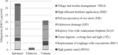
Mitigation technologies for rice cultivation (3C7) such as mitigation drainage (MD) and fall incorporation of rice straw (FIR) will contribute to reducing 14MtCO₂eq/year and 7.2MtCO₂eq/year of emission, which are 10% of agricultural emissions in the three countries in 2030. With regard to managed soils (3C4), high efficiency fertilizer application (HEF) (i.e. split fertilization) is expected to reduce 14MtCO₂eq/year of emissions. With regard to the livestock sector (3A1 and 3A2), 15 MtCO₂eq/year of emission can be reduced. Ten MtCO₂eq/year of the emission would be reduced by Replacement of roughage with concentrates (RRC), which is the greatest contribution mitigation technology for livestocks. In Indonesia, 33 MtCO₂eq/year of emissions can be reduced in total in agriculture in 2030 under 10USD/tCO₂eq. The largest potential technologies are HEF, MD and RRC which would reduce 24MtCO2eq/year. In Malaysia, there is 1.4 MtCO₂eq/year of GHG mitigation in 2030. The largest potential technology is MD which would reduce 0.5 MtCO2eq/year. In Vietnam, 21 MtCO₂eq/year of GHG emissions can be reduced. The largest potential technologies are MD, FIR and RRC which would reduce 13MtCO₂eq/year.

Figure 5 shows the breakdown of total GHG mitigation potentials by technology in agriculture in the three countries under a wide range of AACs in 2030. Higher costs will lead to higher mitigation potentials. There are three types of technologies taking negative or zero cost, which are called “no regret technologies” (AAC is less than 0USD/tCO₂eq): midseason drainage (MM), Dome digester, cooking fuel and light (CFL) and RRC. They will provide 33 MtCO₂eq/year of mitigation potentials.

Figure 5. Greenhouse gas mitigations by technology under different allowable costs for GHG emission mitigations in Indonesia, Malaysia and Vietnam.

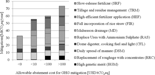
Under 10USD/tCO₂eq of AAC, mitigation potentials in agriculture will be 56MtCO₂eq. Efficient fertilizer application, FIR, RAS and TRM would be applied at 0 to 10USD/tCO₂eq of AAC. Expensive technologies such as slow release fertilizer were not selected under 10USD/tCO₂eq.

Over 100USD/tCO₂eq of AAC, the maximum technical mitigation will be 74 MtCO₂eq/year in agriculture sector. This corresponds to 30% and 49% of agricultural emissions in 2005 and 2030, respectively.

Summary

In this study, GHG emission and mitigations in the AFOLU sector in the three Southeast countries are estimated and evaluated. The findings are as follows:

–

In Indonesia, Malaysia and Vietnam, GHG emissions in agriculture and LULUCF sectors were 149MtCO2eq/year and 1.0GtCO2eq/year in 2005. In the BaU case, the emissions are expected to increase 1.7 and 1.8 times up to 2030. Carbon sink in LULUCF was –525MtCO2eq/year in 2005 and will be –428MtCO2eq/year in 2030 in the BaU case.

•	In the Southeast Asian countries, under 10USD/tCO2eq of AAC, 56MtCO2eq/year of emissions can be reduced in agriculture sectors, which correspond to 38% of the agricultural emissions at the 2005 level.
•	No-regret mitigation technologies: MM and FIR in rice cultivation and RRC are expected to reduce 33MtCO2eq/year in 2030, which corresponds to 22% of agricultural emissions at the 2005 level.