Global mitigation of non-CO₂ greenhouse gases: marginal abatement costs curves and abatement potential through 2030

Abstract

Greenhouse gases (GHGs) other than carbon dioxide (CO₂) play an important role in the effort to understand and address global climate change. Approximately 25% of Global warming potential-weighted GHG emissions in the year 2005 comprise the non-CO₂ GHGs. The report, Global Mitigation of Non-CO₂ Greenhouse Gases: 2010–2030 provides a comprehensive global analysis and resulting data-set of marginal abatement cost curves that illustrate the abatement potential of non-CO₂ GHGs by sector and by region. The basic methodology – a bottom-up, engineering cost approach – builds on the baseline non-CO₂ emissions projections published by EPA, applying abatement options to the emissions baseline in each sector. The results of the analysis are MAC curves that reflect aggregated breakeven prices for implementing abatement options in a given sector and region. Among the key findings of the report is that significant, cost-effective abatement exists from non-CO₂ sources with abatement options that are available today. Without a price signal (i.e. at $0/tCO₂e), the global abatement potential is greater than 1800 million metric tons of CO₂ equivalent. Globally, the energy and agriculture sectors have the greatest potential for abatement. Among the non-CO₂ GHGs, methane has the largest abatement potential. Despite the potential for project level cost savings and environmental benefits, barriers to mitigating non-CO₂ emissions continue to exist. This paper will provide an overview of the methods and key findings of the report.

Keywords:

• Non-CO₂ greenhouse gases
• marginal abatement cost curves
• methane
• nitrous oxide
• hydrofluorocarbons

1. Introduction

Climate change is influenced by a number of social and environmental factors. The change in our Earth’s climate is largely driven by emissions of greenhouse gases (GHGs) to the atmosphere. While some GHG emissions occur through natural processes, the largest share of GHG emissions come from human activities. GHG emissions from anthropogenic sources have increased significantly over a relatively short time frame (~100 years) and are projected to grow appreciably over the next 20 years.

Policy development and planning efforts are underway at all levels of society to identify climate change strategies that effectively reduce future GHG emissions and prepare communities to adapt to the Earth’s changing climate. GHG abatement analysis continues to play an important role in the formation of climate change policy. A large body of research has been dedicated to analyzing ways to reduce carbon dioxide (CO₂) emissions. While this work is critical to developing effective climate policy, other GHG gases can play an important role in the effort to address global climate change. These non-carbon dioxide (non-CO₂) GHGs include methane (CH₄), nitrous oxide (N₂O), and a number of fluorinated gases. While there is consensus within the scientific community that black carbon is contributing to climate change, it is not included in the report due to a lack of comprehensive data on emissions, abatement, and costs.

Non-CO₂ GHGs are more potent than CO₂ (per unit weight) at trapping heat within the atmosphere. Global warming potential (GWP) is the metric that quantifies the heat trapping potential of each GHG relative to that of CO₂. For example, CH₄ has a GWP value of 21¹ over a 100 year time period which means that each molecule of CH₄ released into the atmosphere is 21 more times effective at trapping heat compared to an equivalent unit of CO₂. Some GHGs have relatively short atmospheric lifetimes (e.g. CH₄, black carbon, and some hydrofluorocarbons (HFCs)), while others have much longer atmospheric lifetimes ranging from hundreds to thousands of years. While the scientific community has developed other metrics to compare GHGs, such as the 20 year GWP, the U.S. primarily uses the 100 year GWP. The 20 year GWP, for example, prioritizes gases with shorter lifetimes, such as CH₄, but results in lower GWPs for gases with longer atmospheric lifetimes. Table 1 shows the list of GHG gases with their GWP values that are considered in this report.²

Table 1. GWPs (IPCC second assessment report).

Greenhouse gases	Abbreviation	GWP (100 years)
Carbon dioxide	CO2	1
Methane	CH4	21
Nitrous oxide	N2O	310
Hydro fluorocarbons	HFCs	140–11,700
Sulfur hexafluoride	SF6	23,900

The report, Global Mitigation of Non-CO₂ Greenhouse Gases: 2010–2030 (U.S. EPA, 2013), an update to U.S. EPA (2006), provides a comprehensive global analysis and resulting data-set of marginal abatement cost curves (MACs) that illustrate the abatement potential of non-CO₂ GHGs by sector and by region. The MAC curves allow for improved understanding of the abatement potential for non-CO₂ sources, as well as inclusion on non-CO₂ GHG abatement in economic modeling of multigas abatement strategies. This paper presents the methodology, data sources, and key findings of U.S. EPA (2013) and provides comparison of results to previous studies. In this paper we will focus on the non-agriculture sectors including CH₄ and N₂O from energy, waste, and industrial sources, as well as various fluorinated gases from industrial processes, including sulfur hexafluoride (SF₆), perfluorocarbons (PFCs), and HFCs. Discussion of the agriculture sector related MACs from this report is the focus of another paper, Marginal Abatement Cost Curves for Agricultural Non-CO₂ Emissions Through 2030 (Beach et al. 2015).

2. Background

MACs provide information on the amount of emissions reductions that can be achieved as well as an estimate of the costs of implementing the GHG abatement measures. Figure 1 shows an illustrative MAC. The x-axis shows the quantity of emissions abatement in million metric tons of CO₂e (MtCO₂e), and the y-axis shows the breakeven price in dollars per ton of CO₂ equivalent ($/tCO₂e) required to achieve the level of abatement. Therefore, moving along the curve from left to right, the lowest cost abatement options are adopted first.

Figure 1. Example MAC curve.

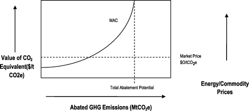
The curve becomes vertical at the point of maximum total abatement potential, which is the sum of all technically feasible abatement options in a sector or region. At this point no additional price signals from GHG credit markets could motivate emissions reductions.

The points on the MAC that appear at or below the zero cost line ($0/tCO₂e) illustrate potentially profitable abatement options. These “below-the-line” amounts represent abatement options that are already cost-effective given the costs and benefits considered (and are sometimes referred to as “no-regret” options) yet have not been implemented. However, there may be nonmonetary barriers that are preventing their adoption.

3. Baselines and projections

The abatement options represented in the MACs of this analysis are applied to the baselines described here. For consistency across regions and sectors the analysis primarily uses the EPA report, Global Anthropogenic Non-CO₂ Greenhouse Gas Emissions: 1990–2030 for baseline emissions and projections. The Global Emissions Report (GER) was published in December of 2012 (U.S. EPA 2012), and uses a combination of country-prepared, publicly-available reports (UNFCCC National Communications) and IPCC Tier 1 methodologies to fill in missing or unavailable data. The basis for the U.S. historical emissions in the GER is the U.S. Inventory of Greenhouse Gases and Sinks published in April of 2011 (U.S. EPA 2011). In some cases, particularly for agricultural emissions, it was necessary to develop separate baselines from which to assess the abatement analyses.

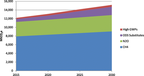
These projections represent a business-as-usual scenario that includes reductions from established sector-specific programs, but not economy-wide programs or commitments. Other projections such as the Representative Concentration Pathways and the Special Report on Emission Scenarios represent a range of socioeconomic drivers and resulting emissions. The EPA projections provide regionally disaggregated non-CO₂ GHG emission projections through 2030 and allow us to develop country level MACs. Figures 2 and 3, depict the historical baseline non-CO₂ GHG emissions (Figure 2) and future projections (Figure 3) used in the report. The fluorinated gases are disaggregated into two categories, ozone depleting substance (ODS) substitutes and other high GWP GHGs. The ODS substitutes are primarily composed of various HFCs emitted from refrigeration and air conditioning, solvent use, foams manufacturing, aerosol product use, and fire protection. The other high GWP GHGs are primarily composed of PFCs, SF₆, and trifluoromethane.

Figure 2. Historical emissions: 1990–2010 (MtCO₂e).

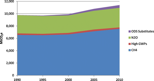
Figure 3. Projected emissions: 2015–2030 (MtCO₂e).

For the agricultural sector, the baseline emissions used in this report were based on crop process model simulations and livestock population data combined with projected crop areas and livestock populations, respectively, from the International Food Policy Research Institute International Model for Policy Analysis of Agricultural Commodities and Trade (IMPACT) model.

3.1. Historical emissions

3.2. Projected emissions

3.3. Baseline emissions for agriculture

Although U.S. EPA (2012) contains estimates of baseline emissions for agricultural sources, alternative baselines were developed for the purposes of the abatement report. The primary rationale was to ensure consistency in the area, number of livestock head, production, and price projections used across the entire agricultural sector. Projections provided by IFPRI from their IMPACT model of global agricultural markets were used to adjust values for agricultural activities and associated emissions over time. In addition, detailed process-based models – Daily Century for croplands and DeNitrification–DeComposition for rice cultivation – were used for both the baseline emissions estimates and the GHG implications of abatement options, thus allowing for a clear identification of baseline management conditions and consistent estimates of changes to those conditions through abatement activities. For emissions associated with livestock, the abatement analysis in this report relies on projections similar to those used in U.S. EPA (2012), but with some differences due to the adjustments made for consistency with IFPRI IMPACT projections across all agricultural sectors. The baseline emissions were also disaggregated by livestock production system and intensity using data provided by the United Nations Food and Agriculture Organization.

4. Methodology

MAC curves are developed for each region and sector by estimating the carbon price at which the present value benefits and costs for each abatement option equilibrates. In conjunction with appropriate baseline and projected emissions for a given sector the results are expressed in terms of absolute reductions of CO₂ equivalents (MtCO₂e). The MACs in this report are constructed from bottom-up average breakeven price calculations. The average breakeven price is calculated for the estimated abatement potential for each abatement option. The options are then ordered in ascending order of breakeven price (cost) and plotted against abatement potential. The resulting MAC is a stepwise function, rather than a smooth curve, as seen in the illustrative MAC below, because each point on the curve represents the breakeven price point for a discrete abatement option (or defined bundle of abatement strategies).

Conceptually, marginal costs are the incremental costs of an additional unit of abatement. However, the abatement cost curves developed here reflect the incremental costs of adopting the next cost-effective abatement option. We estimated the costs and benefits associated with all or nothing adoption of each well-defined abatement practice. However, we did not estimate the marginal costs of incremental changes within each practice (e.g. the net cost associated with an incremental change in paddy rice irrigation). Instead, the MACs developed in this report reflect the average net cost of each option for the achieved reduction – hence the non-continuous, stepwise nature of the curve.

This analysis builds on the approach used in the EMF-21 multigas mitigation study (Weyant & de la Chesnaye 2006) and U.S. EPA (2006). The non-CO₂ emission sources and gases included in this analysis are:

•	coal mining (CH4);
•	oil and natural gas systems (CH4);
•	solid waste management (CH4);
•	wastewater (CH4, N2O);
•	specialized industrial processes (N2O, PFCs, SF6, HFCs); and
•	agriculture (CH4, N2O).

In addition to updating primary drivers in the model, including baseline emissions projections and energy price paths, we updated capital and operation and maintenance (O&M) costs for individual abatement measures, reduction efficiencies for individual measures by country, and developed international adjustment factors used to construct country specific abatement costs and benefits. Further, in the agriculture sector we updated crop process model simulations of changes in crop yields and emissions associated with rice cultivation and cropland soil management. For more information about additional enhancements to the agriculture sectors and the resulting MACs please see Beach et al., “Marginal abatement cost curves for agriculture non-CO₂ emissions through 2030.”

4.1. Abatement option analysis methodology

The abatement option analysis throughout this report was conducted using a common methodology and framework. The abatement analysis for all non-CO₂ gases for agriculture, coal mines, natural gas and oil systems, landfills, wastewater treatment, and nitric and adipic acid production are based on U.S. EPA (2006) and improve upon DeAngelo et al. (2006), Beach et al. (2008), and Delhotal et al. (2006) by incorporating updated abatement technologies, costs, and parameters. These studies provided estimates of potential CH₄ and N₂O emissions reductions from major emitting sectors and quantified costs and benefits of these reductions. Additional data on abatement options, costs, and market penetration come from partner reported data from U.S. EPA non-CO₂ GHG voluntary programs, including the Landfill Methane Outreach Program, Natural Gas STAR, AgSTAR, and the Coalbed Methane Outreach Program.

Given the detailed data available for U.S. sectors, the U.S. regional analysis uses representative facility estimates but then applies the estimates to a highly disaggregated and detailed set of emissions sources for all the major sectors and subsectors. For example, the analysis of the natural gas sector is based on more than 100 emissions sources in that industry, including gas well equipment, pipeline compressors and equipment, and system upsets. Thus, the analysis provides significant detail at the sector and subsector levels.

4.2. Technical characteristics of abatement options

The non-CO₂ abatement options evaluated here are compiled from the studies mentioned above, as well as from the literature relevant for each sector. For each region, either the entire set of sector-specific options or the subset of options determined to be applicable is applied. Options are omitted from individual regions on a case-by-case basis, using either expert knowledge of the region or technical and physical factors (e.g. appropriate climate conditions). In addition, the share or extent of applicability of an option within different regions may vary based on these conditions.

The technical effectiveness of each option is calculated by multiplying the option’s technical applicability by its market share by its reduction efficiency. This yields the percentage of baseline emissions that can be reduced at the national or regional level by a given option. This is then applied to the Emissions stream (MtCO₂e) to which the option is applied to yield the emissions reductions for the abatement option.

Technical applicability accounts for the portion of emissions from a facility or region that an abatement option could feasibly reduce based on its application (Figure 4). For example, if an option applies only to the underground portion of emissions from coal mining, then the technical applicability for the option would be the percentage of emissions from underground mining relative to total emissions from coal mining.

Figure 4. Calculation of potential emission reduction for an abatement option.

^aImplied market share non competing options (i.e. only one options is applicable for an emissions streams) is assumed to add to 100%.

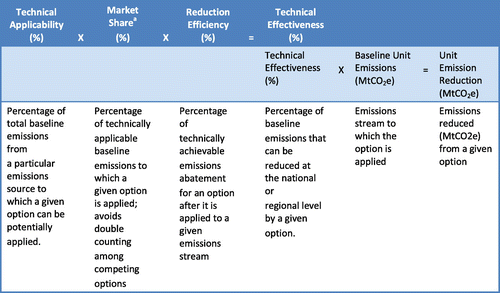
The implied market share of an option is a mathematical adjustment for other qualitative factors that may influence the effectiveness or adoption of an abatement option. For certain energy, waste, and agriculture sectors, it was outside the scope of this analysis to account for adoption feasibility, such as social acceptance and alternative permutations in the sequencing of adoption. For example, if n competing (overlapping) abatement options are available for a single emissions stream, the implied market share of each of the n overlapping options is equal to 1/n. This avoids cumulative reductions of greater than 100% across options.

While this describes the basic application of the implied adoption rate in the energy, waste, and agriculture sectors, this factor is informed by expert insight into the potential market penetration over time in the industrial processes sector. For sectors such as landfills, where market share assumptions are available, customized shares that sum to one are used instead of 1/n.

4.3. Economic characteristics of abatement options

Each abatement option is characterized in terms of its project related costs and benefits or revenues per an abated unit of gas (tCO₂e or tons of emitted gas [e.g. tCH₄]). The benefits or revenues include a carbon value/price expressed as $/tCO₂e, and can include the intrinsic value of the recovered gas, the non-GHG benefits of abatement options (e.g. increase in crop yields), and the value of abating the gas given a GHG price in terms of $/tCO₂e or dollars per metric ton of gas. In addition to the economic benefits associated with a particular abatement option, there may be additional benefits including climate, environmental and health co-benefits. Examples of these additional benefits include climate benefits from reduced GHG emissions, air quality health benefits from CH₄ emission reductions, and the environmental benefits of less nitrogen pollution due to reductions in N₂O emissions. These additional climate, environmental and health benefits are not quantified when evaluating the project related costs and benefits of an abatement option, but should be considered and quantified when assessing larger climate strategies and commitments that may incorporate non-CO₂ related abatement options.

The carbon price at which an option’s benefits equal the costs is referred to as the option’s breakeven price. For each abatement option, the carbon price at which that option becomes economically viable is calculated where the present value of the benefits of the option equals the present value of the costs of implementing the option. A present value analysis of each option is used to determine breakeven abatement costs in a given region. Breakeven calculations are independent of the year the abatement option is implemented but are contingent on the life expectancy of the option. The net present value calculation solves for breakeven price, by equating the present value of the benefits with the present value of the costs of the abatement option.

Costs include capital or one-time costs and O&M or recurring costs. Benefits or revenues from employing an abatement option can include (1) the intrinsic value of the recovered gas (e.g. the value of CH₄ either as natural gas or as electricity/heat, the value of HFC-134a as a refrigerant), (2) non-GHG benefits of abatement options (e.g. compost or digestate for waste diversion options, increases in crop yields), and (3) the value of abating the gas given a GHG price in terms of dollars per tCO₂e or dollars per metric ton of gas (e.g. $/tCH₄, $/tHFC-134a). In most cases, there are two price signals for the abatement of CH₄: one price based on CH₄’s value as energy (because natural gas is 95% CH₄) and one price based on CH₄’s value as a GHG. All cost and benefit values are expressed in constant year 2010 U.S. dollars. This analysis is conducted using a 10% discount rate and a 40% tax rate, however the MAC model allows for the analysis to be conducted at varying discount and tax rates. The 10% discount rate was used for this analysis to model the private investment decision. A discount rate of 3 or 5% could be used to estimate the abatement cost of each option from a social perspective. The 40% tax rate closely approximates the U.S. corporate tax rate and is used in the breakeven calculation to account for depreciation of capital associated with abatement technologies. Using lower discount or tax rates would result in lower breakeven prices for many abatement options. Given the relationship between discount rates, tax rates and breakeven prices, the costs for the abatement options modeled represent conservative estimates.

4.4. Limitations and uncertainties

The MACs represent the average economic potential of abatement technologies in that sector. It is assumed that if an abatement technology is technically feasible in a given region then it will be implemented according to the relevant economic conditions. Therefore, the MACs do not represent the market potential or the social acceptance of a technology. In general the analysis takes a static approach to abatement assessment and excludes indirect emissions reductions and transaction costs. The analysis assumes partial equilibrium conditions that do not represent economic feedbacks from the input or output markets. Further, no assumptions are made regarding a policy environment that might encourage the implementation of abatement options.

Technological change in abatement option characteristics including, availability, reduction efficiency, applicability, and costs is not included in the MAC model. For most sectors, the same set of options are applied in 2020 and 2030 and an option’s parameters are not changed over the lifetime. Indirect emissions reductions are not accounted for in the analysis due to the requirement for additional assumptions about the carbon intensity of electricity in different regions. While there continues to be ongoing work in the area of abatement option transaction costs (Antinori & Sathaye 2007; Rose et al. 2013), given the lack of comprehensive data, this analysis excludes transaction costs.

5. Results and discussion

The results of the analysis are presented as MACs by region and by sector and generally focus on the 2010–2030 time frame. Figure 5 shows the global total aggregate MAC for all non-CO₂ GHGs in 2030. Worldwide, the potential for cost-effective non-CO₂ GHG abatement is significant. In 2030 the projected global non-CO₂ GHG emissions are over 15 GtCO₂e. Without a price signal (i.e. at $0/tCO₂e), the global abatement potential is greater than 1800 MtCO₂e, or 12% of the projected 2030 non-CO₂ GHG emissions. As the break-even price rises, the abatement potential grows. Significant abatement opportunities could be realized in the lower range of break-even prices. For example, the abatement potential at a price of $10/tCO₂e is greater than 3000 MtCO₂e, or 20% of the baseline emissions, and greater than 3600 MtCO₂e or 24% of the baseline emissions at $20/tCO₂e. In the higher range of breakeven prices, the MAC becomes steeper, and less abatement potential exists for each additional increase in price.

Figure 5. Global total aggregate MAC for non-CO₂ GHGs in 2030.

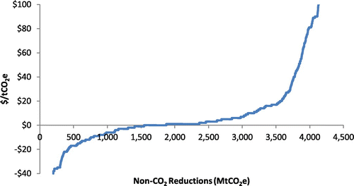
As the figure shows, higher levels of emissions reductions are achievable at higher abatement costs expressed in dollars per metric ton of CO₂ equivalent reduced. The quantity of emissions that can be reduced, or the abatement potential, is constrained by the availability and effectiveness of the abatement measures (emission reduction technologies).

Globally, the sectors with the greatest potential for the abatement of non-CO₂ GHGs are the energy and industrial process sectors, at 1687 and 1597 MtCO₂e of technically feasible reductions in 2030 respectively (Figure 6). While less than that of the energy and industrial process sectors, abatement potential in the agriculture and waste sectors can play an important role, particularly in the absence of a carbon price incentive. The relatively large abatement potential at or below $0/tCO₂e in the energy sector is largely due to the value of CH₄ gas captured or saved, thus making many of the abatement opportunities in this sector cost effective at low or negative carbon prices. It should be noted that despite the potential for project level cost savings (negative cost abatement options) and environmental benefits, barriers to mitigating non-CO₂ emissions, particularly CH₄, continue to exist. These barriers include traditional industry practices and abatement options that are outside of core business practices, regulatory and legal issues, and a continued uncertain investment environment for climate mitigation projects. Non-CO₂ abatement policies, as well as broader climate mitigation strategies, are important and necessary to motivate adoption of abatement measures.

Figure 6. Global 2030 MACs for non-CO₂ GHGs by major sector.

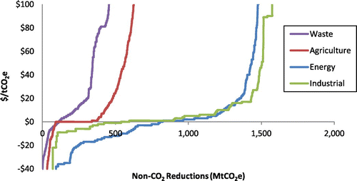
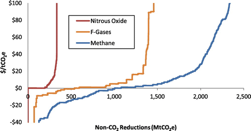
Figure 7 depicts the abatement potential by gas in 2030. CH₄ offers the largest potential for abatement across of all of the non-CO₂ GHGs with over 2300 MtCO₂e of technically feasible reductions available in 2030. The fluorinated industrial gases and N₂O combined offer over 1700 MtCO₂e of technically feasible reductions in the same time period. In addition to the technically feasible reductions, it is worth noting the large volume of cost-effective reductions (reductions at $0/tCO2e) which could be undertaken without the benefit of a carbon price to make the abatement option economically feasible.

Figure 7. Global 2030 MACs by non-CO₂ GHG.

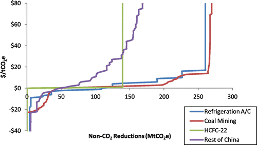
As shown in Figure 8, China and the U.S. are the top two contributors to global abatement potential with cost-effective ($0/tCO₂e) abatement of 249 and 165 MtCO₂e respectively. Total technically feasible abatement for these two regions is 560 and 928 MtCO₂e for China and the U.S. respectively. Taking a closer look at the largest sources of abatement potential in these regions, this analysis shows that Oil/Gas, Refrigeration/AC, Livestock, and Coal offer the greatest opportunities, as shown in Figures 9 and 10.

Figure 8. Global 2030 MACs for non-CO₂ GHGs by major emitting regions.

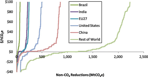
Figure 9. 2030 MACs for United States.

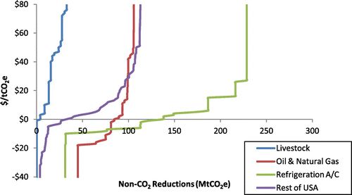
Figure 10. 2030 MACs for China.

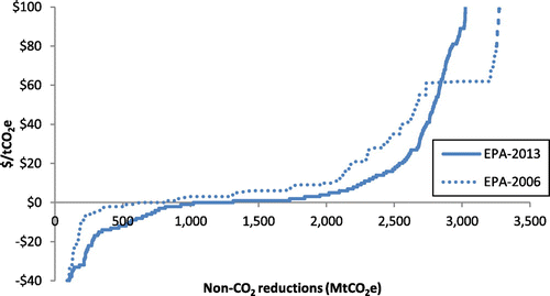
5.1. Comparison to previous studies

The previous U.S. EPA (2006) non-CO₂ GHG MAC study only evaluated abatement potential out through 2020. Comparing 2020 abatement potentials (Figure 11) we find that the 2013 analysis shows 3581 MtCO₂e of technically feasible abatement potential globally, where EPA (2006) showed 3401 MtCO₂e, a difference of 5%.

Figure 11. 2020 MAC for non-CO₂ GHGs – comparison of EPA 2006 and EPA 2013 reports.

As shown in Figure 12, the sectors driving this difference are Agriculture and Waste. In addition, the industrial sector has expanded to include photovoltaic and flat panel display manufacturing. The change in the agriculture sector is related to updated baselines and gas prices, while the change in the landfill sector is attributable to an updated modeling approach that uses actual operating landfills to more accurately account for abatement costs and reductions given real-world parameters.

Figure 12. Comparison of global non-CO₂ MACs in 2020. (a) Energy sector MACs for 2020. (b) Agricultural sector MACs for 2020. (c) Industrial sector MACs for 2020. (d) Waste sector MACs for 2020.

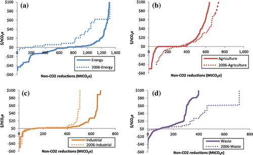
Additional drivers of differences in the abatement potentials shown in these analyses include updated energy prices, and updated capital and O&M costs for abatement measures. Other key model improvements incorporated since the 2006 have also contributed to the difference between the two reports. These model changes include incorporation of more detailed facility level information in the energy, waste, and industrial sectors; the addition of new abatement options in several sectors; updated reduction efficiencies for existing mitigation options; addition of new industrial and waste sub-sectors.

6. Conclusions

This study, which incorporates new data on mitigation technologies, costs, and emissions baselines, alongside a new modeling approach, provides updated and more detailed MACs disaggregated globally for all non-CO₂ GHGs and sectors. The resulting comprehensive data-set of MAC curves allow for improved understanding of the mitigation potential for non-CO₂ sources, as well as inclusion of non-CO₂ GHG mitigation in economic modeling of multigas mitigation strategies. The level of disaggregation provided by this analysis allows end users, including modelers, policy makers, and analysts, flexibility in the way in which the data can be aggregated and incorporated in to models and analysis. Future research on technological change of abatement option characteristics, as well as inquiry in to appropriate transaction costs associated with the implementation of abatement options will result in additional improvements to the MAC analysis and data sets.

Disclosure statement

No potential conflict of interest was reported by the authors.

Notes

1. Based on IPCC Second Assessment Report, 100 year time horizon (IPCC 1996).

2. IPCC Second Assessment Report (SAR) GWPs (IPCC 1996) were used in this report due to the fact that at the time of publication the U.S. official reporting of GHG emissions and projections to the UNFCCC was in SAR GWPs. Future work and analysis will be conducted using Fourth Assessment Report (AR4) GWPs, as the U.S. has since moved to those values for UNFCCC National Communications.

References

- Antinori C, Sathaye J. 2007. Assessing transaction costs of project-based greenhouse gas emissions trading. Lawrence Berkeley National Laboratory (LBNL). Report No. LBNL-57315.
- [IPCC] Intergovernmental Panel for Climate Change. 1996. IPCC guidelines for national greenhouse gas inventories. Three volumes: Vol. 1, reporting instructions; Vol. 2, workbook; Vol. 3, reference manual. Paris: Intergovernmental Panel on Climate Change, United Nations Environmental Programme, Organization for Economic -operation and Development, International Energy Agency.
- Beach RH, Creason J, Ohrel SB, Ragnauth S, Ogle S, Li C. 2015. Marginal abatement cost curves for agricultural non-CO2 emissions through 2030. Manuscript submitted for publication.
- Beach RH, DeAngelo B, Rose S, Li C, Salas W, DelGrosso S. 2008. Mitigation potential and costs for global agricultural greenhouse gas emissions. Agric Econ. 38:109–115.10.1111/agec.2008.38.issue-2
- DeAngelo BJ, Beach RH, Rose S, Salas W, Li C, Del Grosso S, et al. 2006. International agriculture: estimates of non-CO2 and soil carbon marginal mitigation costs. In: Clapp C, editor. The potential cost of global non-CO2 greenhouse gas reduction (EPA Report 430-R-06-005). Washington (DC): U.S. Environmental Protection Agency, Office of Atmospheric Programs. p. V1–V30.
- Delhotal KC, de la Chesnaye FC, Gardiner A, Bates J, Sankovski A. 2006. Mitigation of methane and nitrous oxide emissions from waste, energy and industry. Energy J. Multi-greenhouse gas mitigation and climate policy special issue. 27:45–62.
- Rose SK, Beach R, Calvin K, McCarl B, Petrusa J, Sohngen B, Youngman R, Diamant A, de la Chesnaye F, Edmonds J, et al. 2013. Estimating global greenhouse gas emissions offset supplies: accounting for investment risks and other market realties. Palo Alto (CA): Electric Power Research Institute [EPRI]. Report 1025510.
- U.S. EPA. 2006. Global mitigation of non-CO2 greenhouse gases. Washington (DC): United States Environmental Protection Agency. 430-R-06-005. Available from: http://www.epa.gov/nonco2/econ-inv/international.html
- U.S. EPA. 2011. Inventory of U.S. greenhouse gas emissions and sinks: 1990–2011. Washington (DC): United States Environmental Protection Agency. (April 2013) EPA Report 430-R-13-001.
- U.S. EPA. 2012. Global anthropogenic non-CO2 greenhouse gas emissions: 1990–2030. Washington (DC): United States Environmental Protection Agency. Available from: http://www.epa.gov/nonco2/econ-inv/international.html
- U.S. EPA. 2013. Global mitigation of non-CO2 greenhouse gases: 2010–2030. Washington (DC): United States Environmental Protection Agency. EPA Report 430R13011. Available from: http://epa.gov/climatechange/EPAactivities/economics/nonco2mitigation.html
- Weyant J, de la Chesnaye F, editors. 2006. Multigas mitigation and climate change. Energy J. Multi-greenhouse gas mitigation and climate policy special issue. 27:1–32.