Investigating biodiversity trends in different mitigation scenarios with a national integrated assessment model

ABSTRACT

The inclusion of Sustainable Development Goals (SDGs) in climate mitigation pathways is critical and can be reached by assessing their consequences through the deployment of appropriate indicators to that end. Integrated Assessment Models (IAMs) are important tools for understanding possible impacts caused by adopting new policies. We investigate terrestrial biodiversity trends (life on land: SDG 15) for three different climate mitigation scenarios for Brazil: (1) A scenario compatible with a world that maintains its current policies with current deforestation rates in the Amazon and the Cerrado biomes; (2) A scenario in which Brazil fulfils its Nationally Determined Contribution (NDC); and (3) A scenario compatible with a world that limits warming to 1.5°C. We use the Brazilian Land-Use and Energy System model (BLUES), a national IAM, to show the implications of the transitions involved in the above-mentioned scenarios for the country up to 2050. We conduct a post-processing analysis using consolidated biodiversity indicators to emphasize how different IAM greenhouse gas (GHG) emissions mitigation solutions present distinct positive and negative potential impacts on biodiversity in Brazil. However, our analysis does not consider the impacts associated with climate change, but only the risks imposed by mitigation policies. Our results indicate that biodiversity loss decreases in the scenarios from (1) to (3), implying that stronger climate change mitigation actions could result in smaller biodiversity losses. We conclude that Brazil has the opportunity to align its biodiversity and climate goals through nature-based solutions (NBS), such as forest conservation, restoration, pasture recovery, and the use of crop-pasture and agroforestry systems.

KEYWORDS:

• Integrated assessment models
• biodiversity
• climate mitigation
• land-use
• land-cover
• SDG

1. Introduction

Biodiversity maintenance and climate change are among humanity’s most significant challenges today (e.g. Pievani 2014; Lewis and Maslin 2015). Individually, these issues are already complex. Scientists and decision-makers are looking for ways to reduce the expected increase in global average temperature and other consequences of climate change; simultaneously, they seek to mitigate the loss of biodiversity and other ecosystem services. However, it is crucial that these issues are analysed together, as there are feedbacks between biodiversity loss and climate change mitigation (e.g. Oliver and Morecroft 2014; Aragão et al. 2018). The mutual reinforcement of climate change and biodiversity loss means that the satisfactory resolution of either issue requires consideration of the other (Pörtner et al. 2021). The assessment of the overall trade-offs requires a systemwide modelling approach that connects energy, land and biodiversity.

Changes in the composition of ecosystems have consequences on carbon absorption and storage, and on the dynamics of atmospheric, hydrological and terrestrial cycles, likewise climate change impacts on biodiversity (e.g. Malhi et al. 2008; Bellard et al. 2012; Fajardo et al. 2019; Maxwell et al. 2019; Mahecha et al. 2022). In addition, several climate mitigation measures can, directly and indirectly, affect biodiversity: for example, both Bioenergy with Carbon Capture and Storage (BECCS) and afforestation can negatively impact biodiversity, especially if implemented at scale (Laurance 2013; Ferrante and Fearnside 2020; Pörtner et al. 2021). Here, we contribute to the discussion of the possible interactions between the Sustainable Development Goals of climate action (SDG 13) and life on land (SDG 15), by analysing trends in biodiversity in a megadiverse country in mitigation scenarios.

Brazil is the most biodiverse country in the world (Mittermeier et al. 1997; Butler 2016). Hence, it is worth investigating how climate policies can alter biodiversity in the country. The country has six major biomes, including two global biodiversity hotspots (the Cerrado and the Atlantic Forest) and the world’s largest tropical wetland (the Pantanal) (Brandon et al. 2005; CBD 2022). Additionally, Brazil holds about one-third of the world’s remaining primary tropical rainforests and about two-fifths of the world’s tropical rainforests with low human impact (Krogh 2021). Between one-sixth and one-fifth of the world’s biological diversity is in Brazil, with the most significant number of endemic species (CBD 2022). It has more than 120 thousand invertebrate species, almost 9 thousand vertebrates identified (Instituto Chico Mendes de Conservação da Biodiversidade 2022), and more than 50 thousand recognized flora species (Jardim Botânico do Rio de Janeiro JBRJ 2022). Despite this richness, Brazil is the country with the greatest primary forest loss (Turubanova et al.2018). Land cover change impacts both emissions (e.g. Houghton 2005) and biodiversity (e.g. Vieira et al. 2008), which is reflected in the country’s climate (UNFCCC 2016a) and biodiversity (CBD 2021) agreements. The country’s climate commitments have highlighted the importance of stopping deforestation as a major emission mitigation option (Brazil 2009, 2010; UNFCCC 2016b). Additionally, Brazil’s biodiversity commitments are aligned with the Aichi Biodiversity Targets, including incorporating biodiversity into national and local development and planning processes (CBD 2022).

Integrated assessment models (IAMs) are important tools for an early understanding of possible impacts caused by adopting new policies. IAMs are increasingly used by the climate community, as they are extremely valuable for modelling climate mitigation pathways (e.g.; Weyant 2017; Bauer et al. 2018; Hasegawa et al. 2021; Köberle et al. 2022). The incorporation of biodiversity in IAMs would allow for a better understanding of how climate mitigation scenarios could affect biodiversity. Nevertheless, some methodological difficulties still persist when it comes to trying to incorporate biodiversity into IAMs. IAMs usually operate on large scales – e.g. global, regional, and national – and, although some many IAMs in fact do have sub-national details on the land-use side, especially regarding biophysical parameters (Stehfest et al. 2014; van Vuuren et al. 2021), IAMs usually lack the details of land-use classes and spatial resolution desirable by ecologists. Therefore, it is normally challenging to represent biodiversity variables in IAMs (Verburg et al. 2013; Harfoot et al. 2014). Yet, incorporating biodiversity in an IAM framework through indicators could allow the assessment of climate solutions to be expanded and strengthened in environmental matters. Society as a whole could benefit from the demonstration of the potential impacts of different climate policies on biodiversity (Hill et al. 2016; Kim et al. 2018; Smith et al. 2019; Pörtner et al. 2021).

The “Bending the curve of biodiversity loss” (Leclère et al. 2020) initiative ensembled IAMs and biodiversity models to assess whether and how humanity could reverse the decline in terrestrial biodiversity caused by habitat conversion. The authors of this initiative used four global IAMs to generate projections of habitat loss and degradation for different scenarios to explore pathways that could enable the reversal of biodiversity decrease (Leclère et al. 2020). Despite these efforts, the inclusion of both biodiversity and climate change in low-cost optimization models that could point to the best solutions to both challenges remains incipient. Additionally, national, rather than global, IAMs are more useful to address national policies. In this way, our methodology adds to the work previously done by focusing on a national IAM, facilitating policy making. The present work has two main contributions: (i) it analyses biodiversity trends in policy scenarios for Brazil, and (ii) it includes biodiversity in an integrated analysis framework. A few initiatives to investigate biodiversity trends have been developed using IAMs on a global scale (Heck et al. 2018; Ohashi et al. 2019; Schipper et al. 2020; Leclère et al. 2020), but to the best of our knowledge none at a national scale.

We investigate biodiversity consequences for three different mitigation scenarios for Brazil: (1) a scenario compatible with a world that maintains its current policies with current deforestation rates in the Amazon and the Cerrado biomes (Rochedo et al. 2018); (2) a scenario in which Brazil fulfils its Nationally Determined Contribution (NDC) submitted to the United Nations Framework Convention on Climate Change (UNFCCC); and (3) a scenario compatible with a world that limits warming to 1.5°C. We focus only on mitigation pathways and, as a consequence, we do not include climate change impacts on biodiversity. We use the Brazilian Land-Use and Energy Systems model (BLUES), a national IAM, to show the implications of the transitions involved in the above-mentioned scenarios for the country up to 2050. Given that land-use change is one of the most significant drivers of terrestrial biodiversity loss (Haines-Young 2009; Pereira et al. 2012; IPBES 2019), we explore how these changes could impact biodiversity in Brazil in three policy scenarios. Our methodology, presented in section 2, allows the investigation of biodiversity trends in any future scenario run by the BLUES model. Section 3 presents our results, while section 4 discusses the limitations of our choices and how our results can help the designing of national policies that can align climate action and biodiversity loss reductions.

2. Materials and methods

The methods we use to analyse the impacts of climate scenarios on biodiversity are presented in five subsections. First, we introduce the BLUES model (subsection 2.1); then, we present the biodiversity indicators we use (subsection 2.2.1), followed by the preprocessing of biodiversity datasets to be compatible with BLUES (subsection 2.2.2). Later, we introduce a post-processing methodology to investigate biodiversity in our BLUES scenarios (subsection 2.2.3). We close the methods section by further explaining the three different mitigation scenarios in which we explore biodiversity tendencies (subsection 2.3).

2.1. The BLUES model

BLUES is a process-based bottom-up IAM model representing Brazil in five macro-economic regions and the whole Brazil region. The model is a low-cost, linear programming optimization tool that assumes perfect foresight over the long term. BLUES represents in great detail conventional and climate mitigation technologies, investments, and operation and maintenance costs for the energy, land use, and water use systems (IAMC wiki 2021; IPCC 2022) and has been used in several previous studies (e.g. Rochedo et al. 2018; Lucena et al. 2018; Köberle 2018; Köberle et al. 2020; Império 2020; Oliveira et al. 2020; Müller-Casseres et al. 2021). Assumptions on costs and efficiencies for the energy technologies can be found in Portugal-Pereira et al. (2016) and Rochedo et al. (2018). For the purpose of this current work, the most important features of BLUES are its land use and land-use change representation. BLUES considers 14 land cover classes – savanna, protected savanna, forest, protected forest, cropland, double-crop systems, planted forest, degraded pasture, healthy pasture, crop-pasture systems, agroforestry with Eucalyptus/Pinus, agroforestry with native forest, urban and water – and seven cost categories – A to G (Figure 1).

Figure 1. Land use and land costs categories in BLUES model. (a) Land cover classes at base year; (b) the cost categories used in the BLUES model, with “A” being the lowest cost category and “G” the highest cost category.

Note: Figure a) does not show crop-pasture and agroforestry systems classes because they are not present in the base year, so from the 14 land cover classes in BLUES, figure 1(a) shows 11. Note: costs are based on Köberle (2018).

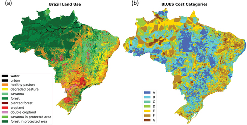
BLUES land cover classes are defined based on the Remote Sensing Center (CSR) map (Soares-Filho et al. 2016) from the Federal University of Minas Gerais (UFMG) and the Laboratory of Image Processing and Geoprocessing (LAPIG) datasets. LAPIG data are used to define pasture allocation and whether it is considered a degraded pasture or not, while CSR provides information about other land cover classes and uses, such as forests, croplands, savannas and others. LAPIG and CSR are combined to generate a unique land cover map for Brazil (Köberle 2018). The BLUES land classes are built as a function of the crop suitability map (Fischer et al. 2021) and a map of travel distance (Weiss 2017). Both are classified in indices that, combined, are used to define BLUES land classes from A, the ones where agricultural activities are cheaper because they present high crop suitability and short travel distance to markets, to G, the most expensive based on Köberle (2018). Within BLUES outputs, we have, for each scenario, projected land-use change, GHG emissions, agricultural products for energy, food and other purposes, and agricultural waste.

BLUES’ conventional and new land-use practices include crop-pasture system and agroforestry, pasture recovery, productivity increase, reforestation, and animal residue management. All these measures are related to changes in costs, inputs and outputs, and, consequently, emissions. For example, in the model, pasture intensification considers an increase of at least 64%, reaching up to 273%, in the cattle stocking rate (Arantes et al. 2018). Pasture improvement increases animal food availability, but there is no consideration of nutritional reinforcement, and extensive livestock production bias is maintained. Additionally, the model assumes that to recover pasture it is necessary an initial investment cost of around 500 US$/ha, spent with the adoption of soil improvement methods through machinery and fertilization. Consequently, the recovered pasture has more carbon stored mainly below ground. Reforestation is the recovery of forest cover in previously deforested areas, but the forest takes 25 years to recover 90% of carbon stocks (maximum biomass recovery) (Angelkorte 2019). Additionally, planted forests can be used to provide the biomass needed to produce advanced biofuels. As a consequence, they are an option to replace fossil fuels with BECCS (Tagomori et al. 2019).

For all scenarios, importing and exporting flows to and from Brazil derive from a global computable general equilibrium (CGE) model named TEA (Total Economy Assessment model). This approach allows Brazil and the world to be aligned in terms of climate policy. BLUES’ international trade is limited by port capacity restrictions. Furthermore, there is no primary biomass trade in the model. TEA represents the production and international trade of agricultural products, industrial goods and energy commodities (Cunha et al. 2020; IAMC wiki 2020). This analysis shows that global agricultural demand maintains its current dietary patterns.

2.2. Biodiversity

2.2.1. Biodiversity indicators

Here, we use three biodiversity indicators: Biodiversity Intactness Index (BII), Human Footprint (HF), and Richness (see datasets; Figure 2). The Intergovernmental Science-Policy Platform on Biodiversity and Ecosystem Services (IPBES) has adopted BII as an important indicator of community composition (IPBES 2019). The index is supported by the PREDICTS project database (Hudson et al. 2014, 2017) and has been used in several studies (e.g. Newbold et al. 2016; Hill et al. 2018; Sanchez-Ortiz et al. 2019; De Palma et al. 2021). HF measures the pressure humans place on ecosystems rather than the human impact on natural systems or their biodiversity. Nevertheless, the HF maps are “better predictors of the range sizes of species than their biological traits, and to be a strong predictor of modern range collapses, the threat status of species, site-scale species richness, and species population size and dispersal ability” (Venter et al. 2016). Both BII and HF are available for the entire global land area (Newbold et al. 2016; Venter et al. 2016). Richness, i.e. the number of species in a local assemblage, is an important index of community structure, and is available for amphibians, birds and mammals for the entire Brazilian territory (Jenkins et al. 2015).

Figure 2. Input data for biodiversity indices and land-use modelling, index values range from 0 to 1 except for Human Footprint (HF) that ranges from 0–50 (no unit). In (a) Biodiversity Intactness Index (BII) in 2010 based on Newbold et al. (2016); (b) HF index in 2009 based on Venter et al. (2016); (c) Normalised Bird Richness Weighted by Human Footprint index (Weighted Bird Richness = Bird Richness *1- HF/100); (d) Normalised Mammal Richness Weighted by Human Footprint index (Weighted Mammal Richness = Mammal Richness *1- HF/100); and (e) Normalised Amphibian Richness Weighted by Human Footprint index (Weighted Amphibian Richness = Amphibian Richness *1- HF/100). Figures (a), (b) and (c) are based on Venter et al. (2016) and Jenkins et al. (2015).

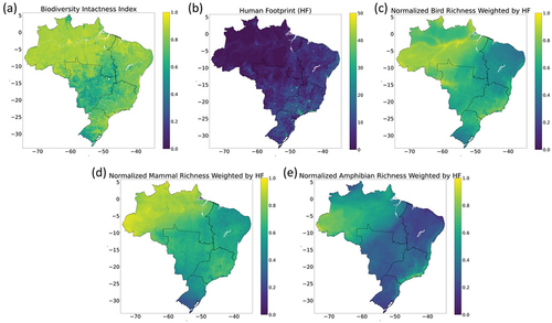
BII represents the area’s average abundance of originally present species relative to the estimated abundance in an undisturbed habitat in 2010 (Scholes and Biggs 2005; Newbold et al. 2016; Leclère et al. 2020). This index presents an estimate with an approximately 1 km² scale of how land-use pressures have affected the abundance of local terrestrial ecological assemblages (Newbold et al. 2016). The index uses four human variables to explain differences in local biodiversity: land use (primary vegetation, secondary vegetation, cropland, pasture and urban), land-use intensity, human population density and distance to the nearest road (Newbold et al. 2016). We normalized the BII data from Newbold et al. (2016).

HF uses eight global variables to estimate cumulative human pressure on the environment in 2009. The considered pressures are as follows: the extent of built environments, cropland, pastureland, human population density, night-time lights, railways, roads, and navigable waterways (Venter et al. 2016). HF is correlated to species extinction risk and to current vegetation biomass relative to that in the same location without human disturbance (Di Marco et al. 2018; Martin et al. 2019).

Finally, richness data are available at https://biodiversitymapping.org/, where polygon range maps are added to create richness maps (Jenkins et al. 2015 – it was last updated in 2017). Brazil has richness data for amphibians, birds and mammals. Richness sampling is labour intensive, and therefore species richness counts are highly sensitive to the number of individuals sampled, and to the number, size, and spatial arrangement of samples (Gotelli and Colwell 2011). Nevertheless, polygon ranges usually do not capture the heterogeneity of suitable and unsuitable habitats within species ranges (Jenkins et al. 2015). To minimize this issue, we decided to weight the richness (WR) index (Equations 1(1) $\mathrm{W}\mathrm{e}\mathrm{i}\mathrm{g}\mathrm{h}\mathrm{t}\mathrm{e}\mathrm{d}\mathrm{A}\mathrm{m}\mathrm{p}\mathrm{h}\mathrm{i}\mathrm{b}\mathrm{i}\mathrm{a}\mathrm{n}\mathrm{R}\mathrm{i}\mathrm{c}\mathrm{h}\mathrm{n}\mathrm{e}\mathrm{s}\mathrm{s}=\mathrm{A}\mathrm{m}\mathrm{p}\mathrm{h}\mathrm{i}\mathrm{b}\mathrm{i}\mathrm{a}\mathrm{n}\mathrm{R}\mathrm{i}\mathrm{c}\mathrm{h}\mathrm{n}\mathrm{e}\mathrm{s}\mathrm{s}\ast \left(1-\hspace{0.17em}\frac{HF}{100}\right)$(1) to 4(4) $\mathrm{W}\mathrm{e}\mathrm{i}\mathrm{g}\mathrm{h}\mathrm{t}\mathrm{e}\mathrm{d}\mathrm{R}\mathrm{i}\mathrm{c}\mathrm{h}\mathrm{n}\mathrm{e}\mathrm{s}\mathrm{s}=\hspace{0.17em}\frac{\mathrm{S}\mathrm{u}\mathrm{m}\mathrm{o}\mathrm{f}\mathrm{W}\mathrm{e}\mathrm{i}\mathrm{g}\mathrm{h}\mathrm{t}\mathrm{e}\mathrm{d}\mathrm{A}\mathrm{m}\mathrm{p}\mathrm{h}\mathrm{i}\mathrm{b}\mathrm{i}\mathrm{a}\mathrm{n},\mathrm{B}\mathrm{i}\mathrm{r}\mathrm{d}\mathrm{a}\mathrm{n}\mathrm{d}\mathrm{M}\mathrm{a}\mathrm{m}\mathrm{m}\mathrm{a}\mathrm{l}\mathrm{R}\mathrm{i}\mathrm{c}\mathrm{h}\mathrm{n}\mathrm{e}\mathrm{s}\mathrm{s}}{3}$(4) ). This methodology aims to add more spatial variability to the richness data based on the assumption that where there is greater anthropogenic pressure there is less biodiversity richness (Newbold et al. 2015). As we wanted to see the trend in richness, we used the combination of richness and HF because changes in HF drive variations in species extinction risk (Di Marco et al. 2018).

(1) $\mathrm{W}\mathrm{e}\mathrm{i}\mathrm{g}\mathrm{h}\mathrm{t}\mathrm{e}\mathrm{d}\mathrm{A}\mathrm{m}\mathrm{p}\mathrm{h}\mathrm{i}\mathrm{b}\mathrm{i}\mathrm{a}\mathrm{n}\mathrm{R}\mathrm{i}\mathrm{c}\mathrm{h}\mathrm{n}\mathrm{e}\mathrm{s}\mathrm{s}=\mathrm{A}\mathrm{m}\mathrm{p}\mathrm{h}\mathrm{i}\mathrm{b}\mathrm{i}\mathrm{a}\mathrm{n}\mathrm{R}\mathrm{i}\mathrm{c}\mathrm{h}\mathrm{n}\mathrm{e}\mathrm{s}\mathrm{s}\ast \left(1-\hspace{0.17em}\frac{HF}{100}\right)$(1)

(2) $\mathrm{W}\mathrm{e}\mathrm{i}\mathrm{g}\mathrm{h}\mathrm{t}\mathrm{e}\mathrm{d}\mathrm{B}\mathrm{i}\mathrm{r}\mathrm{d}\mathrm{R}\mathrm{i}\mathrm{c}\mathrm{h}\mathrm{n}\mathrm{e}\mathrm{s}\mathrm{s}=\mathrm{B}\mathrm{i}\mathrm{r}\mathrm{d}\mathrm{R}\mathrm{i}\mathrm{c}\mathrm{h}\mathrm{n}\mathrm{e}\mathrm{s}\mathrm{s}\ast \left(1-\hspace{0.17em}\frac{HF}{100}\right)$(2)

(3) $\mathrm{W}\mathrm{e}\mathrm{i}\mathrm{g}\mathrm{h}\mathrm{t}\mathrm{e}\mathrm{d}\mathrm{M}\mathrm{a}\mathrm{m}\mathrm{m}\mathrm{a}\mathrm{l}\mathrm{R}\mathrm{i}\mathrm{c}\mathrm{h}\mathrm{n}\mathrm{e}\mathrm{s}\mathrm{s}=\mathrm{M}\mathrm{a}\mathrm{m}\mathrm{m}\mathrm{a}\mathrm{l}\mathrm{R}\mathrm{i}\mathrm{c}\mathrm{h}\mathrm{n}\mathrm{e}\mathrm{s}\mathrm{s}\ast \left(1-\hspace{0.17em}\frac{HF}{100}\right)$(3)

(4) $\mathrm{W}\mathrm{e}\mathrm{i}\mathrm{g}\mathrm{h}\mathrm{t}\mathrm{e}\mathrm{d}\mathrm{R}\mathrm{i}\mathrm{c}\mathrm{h}\mathrm{n}\mathrm{e}\mathrm{s}\mathrm{s}=\hspace{0.17em}\frac{\mathrm{S}\mathrm{u}\mathrm{m}\mathrm{o}\mathrm{f}\mathrm{W}\mathrm{e}\mathrm{i}\mathrm{g}\mathrm{h}\mathrm{t}\mathrm{e}\mathrm{d}\mathrm{A}\mathrm{m}\mathrm{p}\mathrm{h}\mathrm{i}\mathrm{b}\mathrm{i}\mathrm{a}\mathrm{n},\mathrm{B}\mathrm{i}\mathrm{r}\mathrm{d}\mathrm{a}\mathrm{n}\mathrm{d}\mathrm{M}\mathrm{a}\mathrm{m}\mathrm{m}\mathrm{a}\mathrm{l}\mathrm{R}\mathrm{i}\mathrm{c}\mathrm{h}\mathrm{n}\mathrm{e}\mathrm{s}\mathrm{s}}{3}$(4)

2.2.2. Data treatment (preprocessing)

As mentioned before, we used land-use as a surrogate for biodiversity. Therefore, we used the land-cover classes and categories of BLUES to estimate changes in biodiversity in Brazil in mitigation scenarios up to 2050. To do that, we pre-processed biodiversity datasets into indices that could be compatible with BLUES land classes. After making sure all raster grid cells matched (BII, HF and WR spatial data were reprojected and downscaled to the same coordinate system and spatial resolution associated with BLUES base maps, which have a 16.7 arc-second spatial resolution¹), we calculated biodiversity indices for each land-cover class within each cost category class in the five Brazilian macro-economic regions for BLUES base year (2010).

The BLUES base year map has 11 of the 14 land cover classes because crop-pasture and agroforestry systems (2 land cover classes) are a small share of cropland and planted forest areas and did not have specific biodiversity indices. Therefore, to include these three land covers in the analysis, we calculated the biodiversity index for those land cover classes considering a combination of other land cover systems. The biodiversity indices for crop-pasture systems were calculated as an equal proportion of crop and pasture. While for agroforestry, the indices were estimated considering the crop, pasture and forest indices, once agroforestry here is associated with a 30% crop cover, 30% pasture cover and 40% forest share. The forest cover was either eucalyptus small monocultures in crop-livestock-forest with Eucalyptus or crop-livestock-forest with native forest. This is done because although the BLUES base year map does not include crop-pasture and agroforestry land covers, scenarios can contain these land covers.

The combination of the 14 land-cover classes in 7 cost categories² in 5 Brazilian regions resulted in 490 statistical parameters of biodiversity indicators per land-use type. We calculated the mean, median, std, min, max, percentiles 25 and 75 of those 490 land-use types, but the main results are based on the mean values. We also tested other statistical parameters (please see the Supplemental Material), as a way to deal with the natural heterogeneity of the indices. We chose to use the statistical parameters of these 490 land-use types as fixed in the projections up to 2050. Therefore, we are assuming (i) that the biodiversity is homogenously distributed in these land-use types; (ii) the indicators are associated with land-use types in the base year map and no temporal change is considered in biodiversity in each of those 490 land-use types; (iii) biodiversity indices are independent of historical land use, for example, a cropland area in the North will always have the same biodiversity value no matter if this same area was a forest or a pasture in the past.

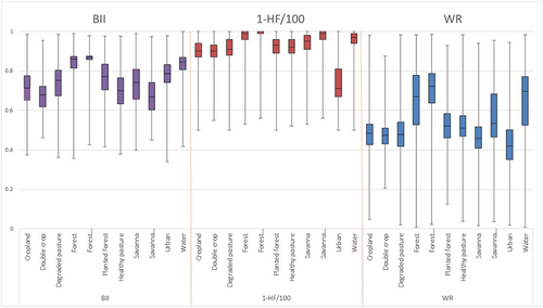
The datasets’ transformations into indices with the same spatial scale as land classes of the BLUES model show interesting patterns (Figure 3). For example, BII within land-use classes shows forests with a wider range but the highest mean, and double-crop with the lowest values. Protected areas in savannas showed a low average, with areas in the Mid-West (MW) and the North (N) driving this effect. Protected forest areas showed the lowest HF and urban areas the highest. The WR shows the highest values for the North and the lowest for the Northeast (NE) region.

Figure 3. Statistical distribution of biodiversity indices for each land cover. HF – Human Footprint, BII – Biodiversity Intactness Index, WR – Weighted Richness.

Note: we analysed the HF on an inverted scale, 1-HF/100, to facilitate the visual comparison between all indices.

Box-plots mark up the maximum, third quartile, median line, first quartile and minimum values in each land cover.

2.2.3. Scenario analysis (post processing)

After pre-processing the biodiversity datasets into indices with the same spatial scale as land classes of the BLUES model, it was possible to analyse biodiversity in scenarios projected in BLUES. Moreover, we conduct a post-processing analysis using BII, HF and WR indices to emphasize how different optimal solutions impact biodiversity in Brazil. We considered a fixed average of biodiversity indices – for each land-cover class within each cost categories class in the five Brazilian macro-economic regions – to extrapolate the results in three future scenarios based on the land-cover change projections. Again, we used the constant land use mean value up to 2050, to project the biodiversity in BLUES scenarios. Thus, our results are based on 490 local averages of those indices, and biodiversity projections are dependent on the current estimation of biodiversity in those areas. Biodiversity indices in a year are calculated considering the sum of the areas of each of the 14 land covers and 7 cost categories and 5 regions multiplied by their given biodiversity index value and divided by the sum of all areas (Equation 5(5) $BiodiversityInde{x}_{year}=\frac{\sum _{x,y,z}{\left(LandAre{a}_{x,y,z}\ast IndexValu{e}_{x,y,z}\right)}_{year}}{\sum _{x,y,z}{\left(LandAre{a}_{x,y,z}\right)}_{year}}$(5) ). It is worth noting that the denominator is a constant value since it is the total value of the area of the Brazilian territory.

(5) $BiodiversityInde{x}_{year}=\frac{\sum _{x,y,z}{\left(LandAre{a}_{x,y,z}\ast IndexValu{e}_{x,y,z}\right)}_{year}}{\sum _{x,y,z}{\left(LandAre{a}_{x,y,z}\right)}_{year}}$(5)

Where:

$x$: represents the set of 14 land covers of the BLUES model (water, urban, degraded pasture, healthy pasture, savanna, protected savanna, forest, protected forest, planted forest, cropland, double crop, crop-livestock systems, agroforestry with planted forest and agroforestry with native forest).

y: represents the set of seven cost categories of the BLUES model (A, B, C, D, E, F and G).

z: represents the set of five macro-economic regions (MW, N, NE, S and SE).

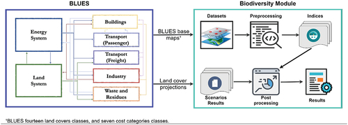
The decision dynamics of BLUES provide the optimal solution based on mathematical constraints that represent a given climate policy. There are additional constraints for limiting land-use change based on historical data. Therefore, the land-use change dynamics are intrinsically hard-linked to the overall optimal decision, which includes mitigation efforts in the energy system. Biodiversity outcomes do not have any constraint capacity on the solution. They were estimated based on model results for the given climate policy narratives. Therefore, incorporating biodiversity indicators (BII, HF and WR) into the BLUES model was performed via a post-processing analysis (Figure 4).

Figure 4. Methodological procedure to integrate biodiversity in the BLUES model. First, data is gathered and processed creating biodiversity indicators for BLUES land cover categories. The scenarios are used to project the biodiversity change based on land cover change. This assessment allows the investigation of possible trends in biodiversity.

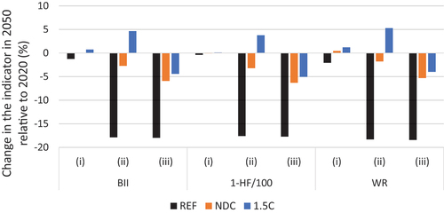
Additionally, we wanted to incorporate the notion that at least part of the loss in biodiversity would never be truly recovered (e.g. Barlow et al. 2007; Audino et al. 2014; Davis et al. 2018). To try to account for that, we carried out a reforestation sensitivity analysis, where (i) is the base-case, in which we considered all the changes in all 14 land cover classes for the quantification of biodiversity indices; and (ii) and (iii) we considered only natural land-cover classes represented in the BLUES model, e.g. savanna and forest (both protected and unprotected). Therefore, for the restoration sensitivity analyses (ii and iii) we consider only changes in savanna and forest land cover classes (4 land-cover classes). In (ii) restoration areas are able to regain biodiversity entirely, and in (iii) restoration areas do not contribute to the increase in biodiversity. Thus, in (iii), if an area is modified from its natural land-cover, its biodiversity index decreases, and even if that area is restored to its original natural land cover class in the future, the biodiversity index remains unchanged. Therefore, in (ii), Equation 5(5) $BiodiversityInde{x}_{year}=\frac{\sum _{x,y,z}{\left(LandAre{a}_{x,y,z}\ast IndexValu{e}_{x,y,z}\right)}_{year}}{\sum _{x,y,z}{\left(LandAre{a}_{x,y,z}\right)}_{year}}$(5) uses only a subset of x, which includes four land covers savanna, protected savanna, forest and protected forest. And in (iii), the biodiversity index value was set as zero for areas of native vegetation recomposition. Biodiversity coefficients were changed manually by inspection of the detailed results from BLUES.

2.3. Scenarios

As mentioned before, we considered three scenarios: a current policies scenario (REF), a world where Brazil fulfils its NDCs (NDC), and a scenario where Brazil fulfils its role in limiting global temperature rise to 1.5°C relative to pre-industrial global temperatures by 2100 (1.5C). REF projects the maintenance of current policies, considering the evolution of trends already present in the country, with no technological disruptions and maintenance of the current deforestation rates in the Amazon and the Cerrado biomes (Rochedo et al. 2018). Current and contracted installed capacities for electricity generation sources, refineries, distilleries, transmission and distribution assets are accounted for, as well as current agricultural production technologies. Some of the applied policies include the Low-Carbon Agriculture program (ABC program – Ministerio da Agricultura, Pecuaria e Abastecimento – MAPA 2021); increasing the percentage of biodiesel in the diesel oil blend, reaching 20% in 2028 (up from 10% as of 2022); international emission reduction targets for the air and maritime sectors established by the International Air Transport Association and the International Maritime Organization, respectively.

On the other hand, the NDC scenario encompasses the compromises already established by the government and the announced goals at COP26. NDC represents efforts to reduce national emissions and adapt to the impacts of climate change (UNFCCC 2023). In terms of mitigation action, Brazil’s first NDC highlights the importance of reducing deforestation, the Brazilian biofuel programs and the role of renewables in the Brazilian energy mix and points to: i) increase the share of sustainable biofuels in the Brazilian energy mix to approximately 18% by 2030; ii) increase environmental governance and achieve zero illegal deforestation while compensating for GHG emissions from legal suppression of vegetation by 2028; iii) reforest 12 million hectares of forests by 2030; iv) strengthen the ABC program, including restoring an additional 15 million hectare of degraded pasturelands and enhancing 5 million hectares of integrated cropland-livestock-forestry systems by 2030; v) achieve 45% of the renewables in the energy mix (primary energy) by 2030 (Brazil 2022). More recently, Brazil informed the UNFCCC that the country aims to reach climate neutrality by 2050 (Brazil 2022), although Brazil’s NDC update has allowed Brazil to emit more GHG by 2030 compared to the previous version (den Elzen et al. 2022). The NDC scenario includes the target of 37% and 50% GHG emission reductions by 2025 and 2030, respectively, compared to 2005 levels, and the achievement of net-zero GHG emissions in 2050.

Furthermore, the 1.5C scenario considers the urgency and need to establish ambitious and effective actions so that the increase in the global average temperature does not exceed 1.5°C by the end of the century, in line with the Paris Agreement. Accordingly, the 1.5C scenario complies with a carbon budget for Brazil, which represents cumulative CO₂ emissions compatible with the 1.5°C global temperature increase target. The remaining carbon budget for Brazil is estimated at 14 GtCO₂ until 2050 (Rochedo et al. 2018; Oliveira et al. 2020).

3. Results

3.1. Energy and land-use results from the different scenarios

The REF scenario represents a Brazil with the maintenance of current policies, considering the evolution of trends already present in the country. REF projects in 2050 an energy mix similar to that of today, where fossil fuels are predominantly used in industry and transport, and deforestation maintains a high current rate. In the 1.5C scenario, fossil fuels are replaced by renewable sources in the energy mix, largely biomass sources. For electricity production, wind power increases, but hydropower does not expand. Electric vehicles and cellulosic biofuels (green diesel and biokerosene) have become common in the transport sector. The production of these biofuels is associated with BECCS, providing negative emissions. Total deforestation stops in the short term and most biofuels are produced in previously degraded pasture areas. The NDC scenario represents a pledge under the process of the Paris Agreement and includes the commitments described previously. The national pledge stays between the REF and the 1.5C scenarios. The food diet is kept constant among the scenarios, and thus food production levels are not modified. Therefore, changes in production levels reflect changes in agricultural commodities related to bioenergy production. Table 1 compiles our general model results.

Table 1. Summary of scenarios results.

	Ref	NDC	1.5C
CO2 emissions in 2050 (MtCO2/yr)	1,600	−600 (Net Zero GHG)	−800
Cumulative CO2 emissions 2020–2050 (GtCO2e)	50.0	15.6	4.5
Energy	14.6	11.5	6.4
Process	3.9	2.8	2.8
LULUCF	31.5	1.3	−4.7
Cumulative N20 emissions 2020–2050 (GtCO2e)	8.4	8.2	8.4
Energy	0.1	0.1	0.1
Process	-	-	-
LULUCF	8.3	8.1	8.3
Cumulative CH4 emissions 2020–2050 (GtCO2e)	21.0	18.5	18.9
Energy	5.0	4.2	4.2
Process	-	-	-
LULUCF	16.0	14.3	14.7
Stopping deforestation year	-	2028	2025
Cumulative land-use changes (2020–2050) (Mha)^a
Recovered pasture	7.4	41.3	37.0
Reforestation	0.0	1.7	41.0
Crop-pasture systems	0.0	4.1	6.4
Agroforestry	6.2	11.2	14.8
Primary biomass to biofuels production in 2050 (EJ/yr)
Woody biomass	2.1	3.4	6.2
Other sources^b	3.0	3.0	3.4
Agricultural residues	0.0	0.3	2.4
Share of renewable sources in the energy mix in 2050	55%	62%	79%
Agricultural production in 2050 (Mt/yr)
Wheat	8.2	8.2	8.2
Fruits	54.9	54.9	54.9
Soybean	221.2	221.2	221.2
Maise	167.1	157.7	156.6
Cereals	5.3	5.3	5.3
Vegetables	11.4	11.4	11.4
Roots	30.1	30.1	30.1
Rice	14.9	14.9	14.9
Pulses	4.1	4.1	4.1
Oilseed	39.1	32.6	21.5
Nuts	1.0	1.0	1.0
Sugarcane	1,264.8	1,261.1	1,373.3
Coffee	4.5	4.5	4.5
Fiber	9.7	9.7	9.7
Woody	72.4	161.3	203.4
Grassy	0.0	0.0	2.9
Bovine meat	13.2	13.2	13.2
Chicken meat	15.2	15.2	15.2
Pork meat	4.7	4.7	4.7
Milk	35.0	35.0	35.0
Eggs	3.4	3.4	3.4

Note: ^afigure S4 shows the evolution of land cover change for the scenarios; ^bmainly sugarcane.

Brazil’s emission trajectories will strongly depend on the environmental governance over deforestation and the enforcement of required actions to meet both its NDC and 1.5°C climate pledges (Rochedo et al. 2018). Deforestation is one of the biggest drivers of the high emission level projected for Brazil in the REF scenario, reaching 1,008 MtCO₂ per year in 2050. In 2020, deforestation and other land-cover changes accounted for 922 MtCO₂ (GWP100 from AR6), representing more than 66% of the country’s annual CO₂ emissions (SEEG 2022). On the other hand, the NDC scenario considers the commitment to end deforestation by 2028, whilst Brazil must revert from positive to negative emissions in the land-use sector as of 2025 to be compatible with a 1.5°C-only warmer world.

The high deforestation rate implied by the REF scenario results in forest loss and an increase in degraded pasture areas. The model does not identify any cost optimal economic activity that justifies the implied deforestation rates. Even though in the BLUES model there are exogenous agricultural demands for food supply and endogenous agricultural products demand for biofuels, the model does not choose to deforest for continuing with its agricultural practices. Results show that there is enough land to expand crop and pasture activities without compromising the forest. However, a high exogenous deforestation rate in the REF scenario is justified due to “land grabbing” that already occurs in Brazil. In order to simulate this practice, we impose the intermediate deforestation rate proposed by Rochedo et al. (2018) in the model.

For the 1.5C scenario, BLUES shows 37 Mha of pasture recovery until 2050, reforestation increase reaching about 41 Mha, an expansion of 7 Mha of crop-pasture systems and almost 15 Mha of combined agroforestry options. While in the NDC scenario, these values are lower, they show similar trajectories, with an expansion of 3 Mha of native forests, 4 Mha of crop-pasture systems and 12 Mha of agroforestry. These scenarios also project an increase in land use for bioenergy production in the region, but this boost arrives in previously degraded pasture areas. Reducing deforestation is crucial to reach 1.5°C, but mitigation options in the energy sector are also needed.

In terms of differences among the Brazilian macro-economic regions, the North region presents 30 Mha and the Midwest 6 Mha of reforested areas by 2050 in the 1.5C scenario. Nevertheless, Savanna is lost in this scenario: 4 Mha in the North, 8 Mha in the Midwest, and 10 Mha in the Northeast. The NDC scenario also presented savanna losses in both the Midwest and the Northeast regions, respectively, 6 Mha and 5 Mha lost by 2050. In the REF scenario, savannas are reduced by 4 Mha and 1 Mha, respectively, in the Midwest and Northeast. The South region is the smallest in the country and the one with lower changes in land use patterns. The South region had 3 Mha of forest loss in the REF scenario, still losing 0.3 Mha in the NDC scenario but increasing by 0.7 Mha in the 1.5C scenario. The Southeast shows less change in forest cover in the REF scenario, with some forest and savanna losses but an increase in 4 Mha of healthy pasture and agroforestry systems. In the NDC scenario, the Southeast shows 9 Mha of pasture recovery but still shows some 2 Mha of Savanna loss. In contrast, the 1.5C scenario points towards a reduction of 18 Mha of degraded pasture and an increase in the healthy pasture (13 Mha), reforestation (2 Mha), agroforestry systems (4 Mha), crop-pasture systems (1 Mha), double crop (1 Mha) and planted forest (1 Mha).

Regarding energy production and use, Brazil currently has a matrix with approximately half of its primary energy coming from renewable sources (48%) and the other half (52%) from fossil sources. However, stringent climate scenarios would require transformations in the energy system. The future primary energy consumption in the REF scenario maintains the same energy sources currently used, while considerable changes occur in the 1.5C scenario. In this latter scenario, there is a decrease in fossil fuel consumption, representing less than 20% of total primary energy in 2050. This decrease is accompanied by an increase in the use of biomass, which has an important role not only for the decarbonization of the energy sector but also for providing negative emissions for the entire economy. The percentages of replacing fossil fuels with advanced biofuels produced from biomass vary for each scenario, reaching an average of 90% replacement by 2050 in the 1.5C scenario. This represents a 300% increase in biofuels production compared to the REF scenario levels. Therefore, the use of advanced biofuels helps to decarbonize some segments of the transport sector, such as air, maritime and freight transport, as well as the industrial sectors. The production of advanced biofuels in the 1.5C scenario would require, in 2050, around 6.2 EJ of woody biomass and 3.4 EJ of other sources, mainly sugarcane, but also 2.4 EJ of agricultural residues. In the NDC scenario, these amounts are lower, corresponding to 3.4 EJ of woody, 3.0 EJ of sugarcane and 0.3 EJ of agricultural residues. Additionally, in the 1.5C scenario, there is an increasing importance of renewable sources, such as solar and wind power, and sugarcane bagasse is used for electricity cogeneration. The NDC is a scenario in which fossil fuels would represent 36% of total primary energy in 2050. In addition, the NDC presents a 50% increase in biofuels production compared to the REF scenario and wind capacity, and generation would greatly expand.

The NDC scenario would neutralize Brazilian GHG emissions by 2050, whereas the 1.5C scenario would neutralize them around 2040, with almost 800 MtCO₂ of negative emissions being generated in 2050. Adding up the carbon emissions for the entire period (2020–2050), the REF scenario would reach cumulative emissions of 43.5 GtCO₂,³ while the NDC scenario would reach cumulative emissions of 15.6 GtCO₂ and the 1.5C scenario would reach only 7.7 GtCO₂ over this same period.

3.2. Scenarios impact on biodiversity

The three indicators analysed in our work showed similar trends in the three scenarios. When considering all the changes in land cover for the quantification of the indices, the lowest biodiversity is projected for 2050 for the REF scenario, a lower loss for the NDC scenario, and a slight increase in biodiversity for the 1.5C scenario. As forests are the land cover with the highest biodiversity indices, biodiversity benefited, mainly, due to the reduction of deforestation (Figure 5). In the REF scenario, the Brazilian BII is 0.86 in 2020 and shows a 1.2% loss in 2050, while the HF increases by 7.6%, and the loss is 2.1% if projected for the WR. The NDC scenario projects no increase in the BII, a 1.2% increase in the HF, and a 0.4% increase in the WR. The 1.5C scenario shows a 0.8% higher BII in 2050 relative to 2020, reducing the human impact by 1.7% and a slight increase in the WR of 1.2%.

Figure 5. Brazilian regional accumulated land-cover change between 2020 and 2050. In a) current policies scenario (REF); b) Nationally Determined Contribution scenario (NDC); and c) 1.5°C scenario (1.5C).

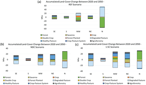
Regional trends demonstrate that the behaviour of the indices is not similar across all regions (Figure 6 and Table 2). The North region, which has most of the Amazon Biome, drives the biodiversity patterns in both 1.5C and NDC scenarios. The savanna loss reflects a regional loss in some biodiversity indices in the Northeast. However, the Midwest reflects the increase in biodiversity promoted by agroforestry. The 1.5C scenario increases HF pressure in the Northeast, the Midwest and the Southeast, while the BII shows an improvement in all regions from 2035 onwards, with considerably higher increases in the Midwest and the North from both reforestation and increases in agroforestry systems. The BII average in the NDC scenario decreases for all regions with the exception of the North, but the national average is pulled up by the North region. The HF decreases in the North and South regions in the NDC scenario, and the WR also includes the Northeast region in the biodiversity recovery. The WR pattern, in this case, is driven by bird richness that only decreases in the Midwest. Mammal richness is reduced both in the Midwest and in the Southeast regions. However, the increase in the North region compensates for losses in the other regions.

Figure 6. Effect of scenario on national biodiversity indices, a) BII – Biodiversity Intactness Index; b) HF – Human Footprint; c) WR – Weighted Richness.

Note: REF – reference scenario; NDC – Nationally Determined Contribution scenario; 1.5 – 1.5°C compliant scenario; we analysed the HF in an inverted scale, as a 1-HF/100, to facilitate the visual comparison between all indices.

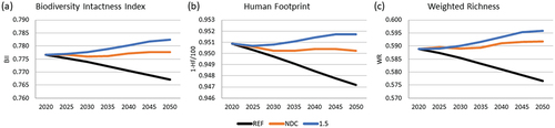
Table 2. Regional Biodiversity indicators, percentage change in 2050 in relation to 2020.

		BII			1-HF/100			WR
		(i)	(ii)	(iii)	(i)	(ii)	(iii)	(i)	(ii)	(iii)
Brazil		−1.2	−17.8	−17.9	−0.4	−17.6	17.7	−2.1	−18.3	−18.4
REF	MW	−1.5	−22.3	−22.4	−0.4	−22.2	−22.2	−0.6	−22.0	−22.0
	N	−1.8	−18.2	−18.3	−0.6	−17.9	−17.9	−3.5	−18.4	−18.4
	NE	−0.3	−6.0	−6.0	−0.1	−5.9	−6.0	0.0	−6.1	−6.1
	S	−0.6	−27.4	−28.2	−0.1	−26.4	−27.3	−0.5	−27.2	−28.0
	SE	−0.1	−36.9	−39.1	−0.3	−37.2	−39.4	−0.2	−37.2	−39.4
Brazil		0.1	−2.7	−5.9	−0.1	−3.2	−6.3	0.4	−1.8	−5.3
NDC	MW	−0.4	−12.2	−12.3	−0.2	−12.9	−13.0	−0.2	−12.6	−12.8
	N	0.4	2.5	−2.1	0.1	2.3	−2.2	0.8	2.6	−2.0
	NE	−0.2	−14.0	−14.0	−0.3	−14.0	−14.0	0.4	−14.0	−14.0
	S	−0.2	−9.5	−10.2	0.0	−9.1	−9.9	0.1	−9.3	−10.1
	SE	−0.1	−20.0	−22.7	−0.2	−20.6	−23.2	−0.2	−20.3	−23.0
Brazil		0.8	4.7	−4.4	0.1	3.8	−5.0	1.2	5.3	−4.0
1.5C	MW	1.0	−0.3	−10.1	0.0	−2.0	−11.9	0.3	−1.6	−11.5
	N	1.1	8.6	−1.1	0.3	8.1	−1.3	1.9	8.7	−1.0
	NE	0.0	−8.4	−12.6	−0.2	−8.9	−12.9	0.4	−8.7	−12.7
	S	0.7	8.1	−0.3	0.1	7.8	−0.3	1.2	8.0	−0.3
	SE	0.1	−3.4	−17.3	−0.1	−5.3	−18.7	−0.1	−4.5	−18.1

Note: REF – Reference scenario; NDC – Nationally Determined Contribution scenario; 1.5–1.5°C compliant scenario; we analysed the HF in an inverted scale. as a 1-HF/100. to facilitate the visual comparison between all indices.

The losses in natural vegetation covers motivated us to perform the additional analyses (ii) and (iii). When biodiversity is not considered in reforestation and agroforestry activities, all indices show a biodiversity loss (Figure 7). The BII of native vegetation was reduced by 18% in the REF scenario, 5.9% in the NDC scenario and increased by 4.4% in the 1.5C scenario. The WR shows a decrease of 18.4%, 5.3% and 4.0%, respectively, in the REF, NDC and 1.5C scenarios in (iii). If reforestation is considered to recover biodiversity (ii), BII in native vegetation in the NDC scenario is 2.7% lower than in 2020 and would increase by 4.7% in the 1.5C scenario. The regional trends show very similar patterns in the (ii) and (iii) for the REF scenario, with all regions losing biodiversity, the loss ranges from around 6% in all indicators for the Northeast region to around 37 in the Southeast. The South, North and Midwest show around 27%, 22% and 18% loss, respectively. For the NDC scenario, the North region highlights the change from considering (ii) or not reforestation (iii). For land cover classes with natural vegetation, the north’s BII in 2050 shows a 2.1% loss when reforestation is not considered (iii) to a 2.6% gain when reforestation is considered (ii) compared to BII in 2020. For the 1.5C scenario, the possibility of regaining biodiversity in natural land cover classes appears in all regions, in the north and south regions, the increase in biodiversity promoted by reforestation and agroforestry compensates for losses in natural vegetation.

Figure 7. Sensitivity analyses, (i) we considered all the changes in land cover for the quantification of biodiversity indices; (ii) we considered only natural land-cover classes in represented in the BLUES model, restoration areas regain biodiversity entirely; and in (iii) restoration areas do not contribute to the increase in biodiversity.

Note: REF – Reference scenario; NDC – Nationally Determined Contribution scenario; 1.5C – 1.5°C compliant scenario

4. Discussion

Our scenario analyses emphasize the need to examine policies related to climate, energy, land-use change and biodiversity. Results show that with more ambitious climate mitigation measures, such as having a 1.5C scenario with more decarbonization efforts by 2050, substantially benefit biodiversity. This positive effect is due to mitigation action since we did not investigate climate change impacts in this study. The descending curve of the BII in the case of the REF scenario follows the results of other studies on a global and regional scale for current policy scenarios with or without the intervention of environmental policies (Biggs et al. 2008; Hill et al. 2018; Heck et al. 2018; Leclère et al. 2020). We also observe that the reversal of this trend is possible through policies and measures that involve the control of deforestation, forest restoration and agroforestry with native species, among other uses, which was claimed and demonstrated by Mace et al. (2018) and Leclère et al. (2020). It is important to recognize the co-dependence of climate change and biodiversity and develop mechanisms to reinforce synergies between them. Moreover, decision-makers must create sustainable planning to minimize the direct and/or indirect impacts of possible trade-offs to these and other SDGs, such as zero hunger (SDG 2), clean water and sanitation (SDG 6) and life below water (SDG 14).

Various nature-based solutions could act both in biodiversity and climate crises (Seddon et al. 2019). Reducing deforestation and promoting the restoration of forest ecosystems are some of the most important measures. However, agroforestry systems, which can act as corridors for some species, and pasture recovery, which would allow for a land-sparing strategy, are also significant (Hernández-Morcillo et al. 2018; Runting et al. 2019). Despite these potential positive consequences of climate action on biodiversity in Brazil, our BLUES model also showed some potential negative impacts. Previous studies have demonstrated concerns related to possible negative effects on biodiversity when implementing climate mitigation measures related to afforestation, bioenergy, and BECCS (Pörtner et al. 2021). The loss of biodiversity in the Northeast associated with the increase in energy production in the region converges on the notion that it is important to guarantee that bioenergy is placed in areas with established high human impact, such as pastures, as opposed to clearing new areas with higher biodiversity indices. Low cattle stocking is a recurrent problem throughout Brazil, and, as such, incentives to increase grazing productivity could result in positive spillover effects for conservation (Stevenson et al. 2013) and bioenergy production (Köberle et al. 2020). The Brazilian government has previously acted on deforestation control (West and Fearnside 2021). Nevertheless, the Brazilian federal government from 2018–2022 reduced environmental laws, which resulted in severe negative impacts on biodiversity, climate, and human well-being (Barbosa et al. 2021). It is impossible to deal with climate change without dealing with tropical forest loss since it is the major source of GHG emissions in Brazil.

The main way of dealing with different sustainability and biodiversity objectives in (process-based) IAMs has been formulating scenarios, which in turn have implications for land use. From there, most authors have followed two pathways: (i) the addition of biodiversity models to calculate their metrics (Leclère, Leclère et al. 2020, Schipper et al., 2019; Ohashi et al. 2019); and (ii) the adoption of nature conservation policies in an area which, when entering as restrictions, can change the model’s energy and climate results, without specific biodiversity metrics (Eitelberg et al. 2016; Frank et al. 2021). The “Bending the curve of biodiversity loss” assess whether and how humanity could reverse the declines in terrestrial biodiversity caused by habitat conversion (Leclère et al. 2020). Our analyses contribute to this literature and demonstrate that to stay within 1.5°C (Paris Agreement goals), it is important to multiple actions. It requires conserving natural vegetation, restoring part of the lost forest and recovering pasture to maintain food production and increase biofuel production, additionally, these measures can help decrease biodiversity loss. In addition, we further analysed changes within the different regions of Brazil, showing that, although some regions have an alignment between biodiversity and climate benefits, other regions should plan carefully for an alignment of climate and biodiversity policies.

An additional issue to consider is how to deal with biodiversity in restoration sites once there is considerable variation in biodiversity recovery after restoration (Rozendaal et al. 2019; Atkinson et al. 2022). In all our scenarios, biodiversity decreases only when we consider our land cover classes representing natural vegetation without considering biodiversity recovery (iii). In the 1.5C scenario, our scenario with the highest reforestation rate, biodiversity loss is driven by savanna loss, but when the recovery of biodiversity is considered (ii), the increase in native agroforestry and reforestation compensates the loss in the aggregated national indicators. Reforestation is important for biodiversity, but there is no substitution for natural habitat conservation (e.g. Gibson et al. 2011; Kemppinen et al. 2020). It is essential to conserve intact tropical forests to protect endemic species (Gibson et al. 2011; Watson et al. 2018).

Additionally, tropical forest protection is a key climate mitigation solution (Seymour and Busch 2016; Griscom et al. 2017), and old and large trees hold a disproportionate stock of carbon (Stephenson et al. 2014; Lutz et al. 2018). Therefore, it is always important to remind stakeholders that “schemes that allow trading the immediate loss of existing habitat for restoration projects will, at best, result in time lags in the availability of habitat that increases extinction risks, or at worst, fail to achieve the offset at all” (Bekessy et al. 2010). We address the limitation of the IAM assumption that restoration will have the same biodiversity value as the natural vegetation by running comparing (ii) restoration areas are able to regain biodiversity entirely and (iii) restoration areas do not contribute to the increase in biodiversity. We recognize, however, that the truth is likely to occur between (ii) and (iii) and is influenced by time.

In terms of the limitations of this study, firstly, we need to point out some possible issues related to the measures we choose to estimate biodiversity. We choose three well-established indicators but, in addition to their errors, using these indicators with our land classes can bring further deviations. Species richness maps can be very different depending on data sources even in relatively well-studied areas (Graham and Hijmans 2006). Additionally, it is common for sampling mechanisms to be biased, whether concerning space and taxonomic groups or affecting the generated biological diversity patterns (Jenkins et al. 2015). Sometimes, due to the low density of samples, the value of the sampling point is extrapolated to a much larger region, which makes further manipulation of data at smaller scales more complicated (Jenkins et al. 2015). In general, observations, indicators and estimates regarding the richness and abundance of terrestrial species are concentrated in temperate regions (Purvis et al. 2018). BII biodiversity data and estimates modelled are geographically unbalanced. It is well known that economically developed and temperate regions present a greater number of observations and studies, while tropical and economically less developed regions, such as Brazil, are under-represented (Akçakaya et al. 2016; Purvis et al. 2018). Plus, BII was previously criticized for underestimating losses (Rouget et al. 2006; Biggs et al. 2008; Martin et al. 2019) which could be a result of coarse land-use estimates or the use of baseline sites that may already have received considerable human impact (Newbold et al. 2019). However, the use of BII has become increasingly widespread in the IAM community (Chrysafi et al. 2022; Soergel et al. 2021; Mishra et al. 2022).

Moreover, regarding its use over long periods, it is reported that BII has limitations in capturing impacts that occur in the long term, such as habitat fragmentation (Scholes and Biggs 2005). Furthermore, the validation process of HF showed higher false-negative rates; in other words, HF also under-estimated human pressures (Venter et al. 2016). Additionally, the HF map is based on spatially explicit land cover, and we used BLUES land cover classes to process the HF dataset further to facilitate future projections based on BLUES land-use change. Notwithstanding that both land cover information differ and the HF map was created for 2009; potential mismatches could further underestimate HF impact within BLUES land cover classes. Therefore, an important consideration is that we are probably underestimating biodiversity loss. Nevertheless, the three biodiversity indicators showed the same trend in the different scenarios, where the NDC and the 1.5C scenarios showed a considerable reduction in biodiversity loss in relation to the REF scenario. We opted to use only freely available datasets that provide global information to facilitate the replication of our study so that other national IAMs can also apply this same approach.

Another limitation is using the mean of biodiversity indicators within BLUES land cover and land cost classes, although the main findings did not change when we tested other statistical parameters (supplemental material). A substantial simplification of the representation of land use and land cover is inevitable in IAMs due to the spatial extent and computational complexity of these models (Titeux et al. 2016). Thus, we estimated the change in biodiversity considering only the land-use projections from BLUES based on the 490 local averages. Nevertheless, we recognize that the variability of biodiversity trends is much wider. Additionally, although land-use change is one of the largest drivers of terrestrial biodiversity loss (Pereira et al. 2012; IPBES 2019), other drivers, such as hunting, the introduction of exotic species and pollution, are also important (IPBES 2019). Climate change has rapidly risen from an emerging driver of biodiversity change (Pereira et al. 2012) to one of the most studied issues related to biodiversity loss to become likely a major pressure on biodiversity in the coming decades. Climate change pressure could drive more than 10% net loss of species in most of Brazilian territory (Newbold 2018). Despite IAMs being widely used in the climate literature, they tend to deal better with mitigation than adaptation policies and climate impacts (Riahi et al. 2022). Likewise, here we only dealt with mitigation pathways. Therefore, even further biodiversity losses should be expected in all scenarios because of climate change consequences, where scenarios with higher emissions should suffer the most.

5. Conclusion

We show biodiversity trends for three climate mitigation scenarios for Brazil. We conclude that climate action can help biodiversity in Brazil. Our results highlight that Brazil has the opportunity to align its biodiversity and climate goals through nature-based solutions, such as forest conservation, restoration, pasture recovery, and the use of agroforestry systems as corridors. Additionally, IAMs can show how much biofuel production could potentially be increased without necessarily spilling over to natural vegetation areas. However, further study of the spatialization of actions, particularly regarding biofuels, is essential. Here, we gave one step to approximate the biodiversity and IAMs “worlds”.

Nevertheless, much more work is necessary, so that the complexity, representativeness and terminology of biodiversity can be fully incorporated into IAMs. IAMs are constantly improving, which is the case with the BLUES model. This study constitutes the beginning of a framework for assessing biodiversity in IAMs on a national and regional scale. As previously indicated, to improve our analysis, it is necessary to expand the scales and even have the possibility of having better conclusions at the regional, and even biome levels. Future work should endogenously integrate biodiversity aspects into IAMs structure, contributing to better evaluating integrated and cross-sectional SDGs achievements. Therefore, our next steps include adding constraints on land-use changes and land use to safeguard biodiversity in BLUES, inspired by conservation planning and spatial prioritization (e.g. Faleiro and Loyola 2013; Fonseca and Venticinque 2018; MMA 2018; Strassburg et al. 2020). Simulations of scenarios with different spatial prioritization could be useful to assess the feasibility of future pathways for meeting the SDGs and the Paris Agreement. Finally, it is worth highlighting the need to formulate national policies incorporating the interdependence of the energy transition, climate change and biodiversity.

Highlights

• A post-processing analysis to investigate biodiversity trends in Brazil was performed – Three mitigation scenarios were explored using a national IAM

• Different biodiversity indicators were used, and they showed similar trends over time – Results showed that strong climate mitigation can have limited biodiversity losses

• Brazil can align its biodiversity and climate goals through nature-based solutions

Acknowledgments

This work has received funding from the European Union’s Horizon 2020 research and innovation programme under grant agreement nº 821471 (ENGAGE) and grant agreement nº 821124 (NAVIGATE). Additionally, the authors would also like to acknowledge the support of the Coordenação de Aperfeiçoamento de Pessoal de Nível Superior - Brasil (CAPES) - Finance Code 001, the National Council for Scientific and Technological Development (CNPq, Brazil) and the National Institute of Science and Technology (INCT, Brazil). We would also like to thank the anonymous reviewers that helped us improve the manuscript considerable.

Disclosure statement

No potential conflict of interest was reported by the author(s).

Data availability statement

The authors confirm that the data supporting the findings of this study are available within the article [and/or] its supplementary materials.

Supplementary material

Supplemental data for this article can be accessed online at https://doi.org/10.1080/1943815X.2023.2239323

Additional information

Funding

The work was supported by the Conselho Nacional de Desenvolvimento Científico e Tecnológico Coordenação de Aperfeiçoamento de Pessoal de Nível Superior .

Notes

1. It is approximately 516 metres x 516 metres in the Equator.

2. The cost categories in BLUES vary from A to F, where A is the region with lowest costs for any culture while F is the most expensive one.

3. GtCO₂ = Billion tonnes of CO₂.

References

- Akçakaya HR, Pereira HM, Canziani CG, Mbow A, Mori A, Palomo MG, Soberón J, Thuiller W, Yachi S. 2016. Improving the rigour and usefulness of scenarios and models through ongoing evaluation and refinement. In: Ferrier S, Ninan KN, Leadley P, Alkemade R, Acosta LA, Akçakaya HR, Brotons L, Cheung WWL, Christensen V, Harhash KA, KabuboMariara J, Lundquist C, Obersteiner M, Pereira HM, Peterson G, Pichs-Madruga R, Ravindranath N, Rondinini C, and Wintle BA editors. The methodological assessment report on scenarios and models of biodiversity and ecosystem services. Secretariat of the Intergovernmental Science. Secretariat of the Intergovernmental SciencePolicy Platform for Biodiversity and Ecosystem Services Bonn, Germany: IPBES. p. 348.
- Angelkorte GB 2019. Modelagem do Setor Agropecuário Dentro de Modelo de Análise Integrada Brasileiro. UFRJ,[s. l.]. http://www.ppe.ufrj.br/images/publicações/mestrado/DISSERTAÇÃO_-_GERD_ANGELKORTE_Versão_FINAL.pdf.
- Aragão LEOC, Anderson LO, Fonseca MG, Rosan TM, Vedovato LB, Wagner FH, Silva CVJ, Silva Junior CHL, Arai E, Aguiar AP, et al. 2018. 21st Century drought-related fires counteract the decline of Amazon deforestation carbon emissions. Nat Commun. 9(1):536. doi:10.1038/s41467-017-02771-y.
- Arantes A, Couto V, Sano E, Ferreira L. 2018. Livestock intensification potential in Brazil based on agricultural census and satellite data analysis. Pesq Agropec Bras. 53(9):1053–28. doi:10.1590/S0100-204X2018000900009.
- Atkinson J, Brudvig LA, Mallen‐Cooper M, Nakagawa S, Moles AT, Bonser SP, Crowther TTerrestrial ecosystem restoration increases biodiversity and reduces its variability, but not to reference levels: A global meta‐analysisEcol Lett20222022 Jul; 252571725–1737. doi:10.1111/ele.14025
- Audino LD, Louzada J, Comita L. 2014. Dung beetles as indicators of tropical forest restoration success: is it possible to recover species and functional diversity? Biol Conserv. 169:248–257. doi:10.1016/j.biocon.2013.11.023.
- Barbosa LG, Alves MAS, Grelle CEV. 2021. Actions against sustainability: Dismantling of the environmental policies in Brazil. Land Use Policy. 104:105384. doi:10.1016/j.landusepol.2021.105384.
- Barlow J, Gardner TA, Araujo IS, Ávila-Pires TC, Bonaldo AB, Costa JE, Peres CA, Ferreira LV, Hawes J, Hernandez MIM. 2007. Quantifying the biodiversity value of tropical primary, secondary, and plantation forests. Proc Natl Acad Sci USA. 104(47):18555–18560. doi:10.1073/pnas.0703333104.
- Bauer N, Rose SK, Fujimori S, van Vuuren DP, Weyant J, Wise M, Cui Y, Daioglou V, Gidden MJ, Kato E, et al. 2018. Global energy sector emission reductions and bioenergy use: overview of the bioenergy demand phase of the EMF-33 model comparison. Clim Change. 163(3):1553–1568. doi:10.1007/s10584-018-2226-y.
- Bekessy SA, Wintle BA, Lindenmayer DB, Mccarthy MA, Colyvan M, Burgman MA, Possingham HP. 2010. The biodiversity bank cannot be a lending bank. Conserv Lett. 3(3):151–158. doi:10.1111/j.1755-263X.2010.00110.x.
- Bellard C, Bertelsmeier C, Leadley P, Thruiller W, Courchamp F. 2012. Impacts of climate change on the future of biodiversity. Ecol Lett. 15(4):365–377. doi:10.1111/j.1461-0248.2011.01736.x.
- Biggs R, Simons H, Bakkenes M, Scholes RJ, Eickhout B, van Vuuren D, Alkemade R. 2008. Scenarios of biodiversity loss in southern Africa in the 21st century. Glob Environ Chang. 18:296–309. doi:10.1016/j.gloenvcha.2008.02.001.
- Brandon K, Da Fonseca GA, Rylands AB, Da Silva JMC. 2005. Special section: Brazilian Conservation: challenges and opportunities. Conserv Biol. 19(3):595–600. doi:10.1111/j.1523-1739.2005.00710.x.
- Brazil. 2009. Law Nº 12.187, [accessed 2009 December 29]. http://www.planalto.gov.br/ccivil_03/_ato2007-2010/2009/lei/l12187.htm
- Brazil. 2010. Decree Nº 6527, [accessed 2010 August 1]. http://www.planalto.gov.br/ccivil_03/_Ato2007-2010/2008/Decreto/D6527.htm
- Brazil. 2022. Nationally Determined Contribution. Jul 2023. https://unfccc.int/sites/default/files/NDC/2022-06/Updated%20-%20First%20NDC%20-%20%20FINAL%20-%20PDF.pdf
- Brazil. 2022. Federative Republic of Nationally Determined Contribution. Available at: https://unfccc.int/sites/default/files/NDC/2022-06/Updated%20-%20First%20NDC%20-%20%20FINAL%20-%20PDF.pdf.
- Butler RA 2016. The top 10 most biodiverse countries. In https://rainforests.mongabay.com/03highest_biodiversity.htmhttps://news.mongabay.com/2016/05/top-10-biodiverse-countries/amp/?print. Access: Dec 2021]. https://rainforests.mongabay.com/03highest_biodiversity.htmhttps://news.mongabay.com/2016/05/top-10-biodiverse-countries/amp/?print
- CBD. 2021. Parties to the nagoya protocol. https://www.cbd.int/abs/nagoya-protocol/signatories/
- CBD. 2022. Brazil- main details. https://www.cbd.int/countries/profile/?country=br#facts
- Chrysafi A. 2022. Quantifying Earth system interactions for sustainable food production via expert elicitation. Nat Sustain. 5(10):830–842. doi:10.1038/s41893-022-00940-6.
- Cunha B, Garrafa R, Gurgel A 2020. TEA model documentation. Working Paper 520. FGV AGRO Nº 001. Available at: https://bibliotecadigital.fgv.br/dspace;handle/bitstream/handle/10438/28756/TD/20520/20-/20FGVAGRO.pdf?sequence=1
- Davis M, Faurby S, Svenning JC. 2018. Mammal diversity will take millions of years to recover from the current biodiversity crisis. Proc Natl Acad Sci. 115(44):11262–11267. doi:10.1073/pnas.1804906115.
- den Elzen M. 2022. Updated nationally determined contributions collectively raise ambition levels but need strengthening further to keep Paris goals within reach. Mitig Adapt Strateg Glob Change. 27(5). doi:10.1007/s11027-022-10008-7.
- De Palma A, Hoskins A, Gonzalez RE, Börger L, Newbold T, Sanchez-Ortiz K, Ferrier S, Purvis A. 2021. Annual changes in the biodiversity intactness index in tropical and subtropical forest biomes, 2001–2012. Sci Rep. 11(1):20249. doi:10.1038/s41598-021-98811-1.
- Di Marco M, Venter O, Possingham HP, Watson JE. 2018. Changes in human footprint drive changes in species extinction risk. Nat Commun. 9(1):1–9. doi:10.1038/s41467-018-07049-5.
- Eitelberg DA, van Vliet J, Doelman JC, Stehfest E, Verburg PH. 2016. Demand for biodiversity protection and carbon storage as drivers of global land change scenarios, Glob. Environ Chang. 40:101e111. doi:10.1016/j.gloenvcha.2016.06.014.
- Fajardo A, McIntire EJB, Olson ME. 2019. When short stature is an asset in trees. Trends Ecol Evol. 34(3):193–199. doi:10.1016/j.tree.2018.10.011.
- Faleiro FAMV, Loyola RD. 2013. Socioeconomic and political trade-offs in biodiversity conservation: a case study of the cerrado biodiversity hotspot, Brazil. Diversity Distrib. 19(8):977–987. doi:10.1111/ddi.12072.
- Ferrante L, Fearnside PM. 2020. The Amazon: biofuels plan will drive deforestation. Nature. 577(7789):170–170. doi:10.1038/d41586-020-00005-8.
- Fischer G, Nachtergaele FO, van Velthuizen HT, Chiozza F, Franceschini G, Henry M, Muchoney D, Tramberend S 2021. Global Agro-Ecological Zones v4 – Model documentation. Rome, Italy: FAO. p. 286. 78-92-5-134426-2. doi:10.4060/cb4744en.
- Fonseca CR, Venticinque EM. 2018. Biodiversity conservation gaps in Brazil: A role for systematic conservation planning. Perspect Ecol Conserv. 16(2):61–67. doi:10.1016/j.pecon.2018.03.001.
- Frank S, Gusti M, Havlik P, Lauri P, DiFulvio F, Forsell N, Hasegawa T, Krisztin T, Palazzo A, Valin H. 2021. Land-based climate change mitigation potentials within the agenda for sustainable development. Environ Res Lett. 16(2):024006. doi:10.1088/1748-9326/abc58a.
- Gibson L, Lee TM, Koh LP, Brook BW, Gardner TA, Barlow J, Sodhi NS, Bradshaw CJA, Laurance WF, Lovejoy TE. 2011. Primary forests are irreplaceable for sustaining tropical biodiversity. Nature. 478(7369):378–381. doi:10.1038/nature10425.
- Gotelli NJ, Colwell RK. 2011. Estimating species richness. Biological Diversity: Frontiers In Measurement And Assessment. 12(39–54):35.
- Graham CH, Hijmans RJ. 2006. A comparison of methods for mapping species ranges and species richness. Global Ecol Biogeogr. 15(6):578–587. doi:10.1111/j.1466-8238.2006.00257.x.
- Griscom BW, Adams J, Ellis PW, Houghton RA, Lomax G, Miteva DA, Fargione J, Shoch D, Siikamäki JV, Smith P. 2017. Natural climate solutions. Proc Natl Acad Sci USA. 114(44):11645–11650. doi:10.1073/pnas.1710465114.
- Haines-Young R. 2009. Land use and biodiversity relationships. Land Use Policy. 26:S178–S186. doi:10.1016/j.landusepol.2009.08.009.
- Harfoot M, Tittensor DP, Newbold T, McInerny G, Smith MJ, Scharlemann JPW. 2014. Integrated assessment models for ecologists: The present and the future. Global Ecol Biogeogr. 23(2):124–143. doi:10.1111/geb.12100.
- Hasegawa T, Fujimori S, Frank S, Humpenöder F, Bertram C, Després J, Drouet L, Emmerling J, Gusti M, Harmsen M, et al. 2021. Land-based implications of early climate actions without global net-negative emissions. Nat Sustain. 4(12):1052–1059. doi:10.1038/s41893-021-00772-w.
- Heck V, Gerten D, Lucht W, Popp A, 2018. Biomass-based negative emissions difficult to reconcile with planetary boundaries. Nat Clim Chang. 8(2):151–155. doi:10.1038/s41558-017-0064-y.
- Hernández-Morcillo M, Burgess P, Mirck J, Pantera A, Plieninger T. 2018. Scanning agroforestry-based solutions for climate change mitigation and adaptation in Europe. Environ Science & Policy. 80:44–52. doi:10.1016/j.envsci.2017.11.013.
- Hill SLL, Gonzalez R, Sanchez-Ortiz K, Caton E, Espinoza F, Newbold T, Tylianakis J, Scharlemann JPW, De Palma A, Purvis A. 2018. Worldwide impacts of past and projected future land-use change on local species richness and the biodiversity intactness index. bioRxiv. doi:10.1101/311787.
- Hill S, Harfoot M, Purvis A, Purves D, Collen B, Newbold T, Burgess ND, Mace GM. 2016. Reconciling biodiversity indicators to guide understanding and action. Conserv Lett. 9(6):405–412. doi:10.1111/conl.12291.
- Houghton RA. 2005. Tropical deforestation as a source of greenhouse gas emissions. In: Moutinho P Schwartzman S, editors Tropical Deforestation and climate change. Belém, Brazil: Instituto de Pesquisa Ambiental da Amazonia; pp. 13–21.
- Hudson LN, Newbold T, Contu S, Hill SLL, Lysenko I, De Palma A, Phillips HRP, Alhusseini TI, Bedford FE, Bennett DJ, et al. 2017. The database of the PREDICTS (projecting responses of ecological diversity in changing terrestrial systems) project. Ecol Evol. 7(1):145–188. doi:10.1002/ece3.2579.
- Hudson LN, Newbold T, Contu S, Hill SLL, Lysenko I, De Palma A, Phillips HRP, Senior RA, Bennett DJ, Booth H, et al. 2014. The PREDICTS database: a global database of how local terrestrial biodiversity responds to human impacts. Ecol Evol. 4(24):4701–4735. doi:10.1002/ece3.1303.
- IAMC wiki. 2020. Model documentation - COFFEE-TEA. https://www.iamcdocumentation.eu/index.php/Model_Documentation_-_COFFEE-TEA
- IAMC wiki. 2021. Model documentation - BLUES. https://www.iamcdocumentation.eu/index.php/Model_Documentation_-_BLUES
- Império MMTS 2020. Atmospheric pollution and global climate change nexus in an integrated assessment model for Brazil. Universidade Federal do Rio de Janeiro. http://www.ppe.ufrj.br/images/publica%C3%A7%C3%B5es/doutorado/Tese_MarianaImp%C3%A9rio.pdf
- Instituto Chico Mendes de Conservação da Biodiversidade. ICMBio. Accessed 10 Jun 2022 https://www.icmbio.gov.br/portal/faunabrasileira
- IPBES. 2019. Global assessment report on biodiversity and ecosystem services of the intergovernmental science-policy platform on biodiversity and ecosystem services (Version 1). Zenodo. doi:10.5281/zenodo.5657041.
- IPCC 2022. Annex III: scenarios and modelling methods. In: Guivarch C, Kriegler E, Portugal-Pereira J, Bosetti V, Edmonds J, Fischedick M, Havlík P, Jaramillo P, Krey V, Lecocq F, Lucena A, Meinshausen M, Mirasgedis S, O’Neill B, Peters GP, Rogelj J, Rose S, Saheb Y, Strbac G, Strømman AH, van Vuuren DP, Zhou N (editors)]. In IPCC, 2022: climate change 2022: mitigation of climate change. Contribution of working group III to the sixth assessment report of the intergovernmental panel on climate change [Shukla PR, Skea J, Slade R, Al Khourdajie A, van Diemen R, McCollum D, Pathak M, Some S, Vyas P, Fradera R, Belkacemi M, Hasija A, Lisboa G, Luz S, Malley Jeditors. Cambridge University Press:Cambridge, UK and New York, NY, USA; doi:10.1017/9781009157926.022.
- Jardim Botânico do Rio de Janeiro (JBRJ). Flora e Funga do Brasil. [Accessed 2022 Jun 10]. http://floradobrasil.jbrj.gov.br/
- Jenkins CN, Alves MAS, Uezu A, Vale MM, Stow A. 2015. Patterns of vertebrate diversity and protection in Brazil. PLoS One. 10(12):e0145064. https://biodiversitymapping.org/. doi:10.1371/journal.pone.0145064.
- Kemppinen KM, Collins PM, Hole DG, Wolf C, Ripple WJ, Gerber LR. 2020. Global reforestation and biodiversity conservation. Conserv Biol. 34(5):1221–1228. doi:10.1111/cobi.13478.
- Kim H, Rosa I, Alkemade R, Leadley P, Hurtt G, Popp A, Pereira HM, Anthoni P, Arneth A, Baisero D. 2018. A protocol for an intercomparison of biodiversity and ecosystem services models using harmonised land-use and climate scenarios. Geosci Model Dev. 11(11):4537–4562. doi:10.5194/gmd-11-4537-2018.
- Köberle A. 2018. Implementation of land use in an energy system model to study the long-term impacts of bioenergy in Brazil and its sensitivity to the choice of agricultural greenhouse gas emission factors. Universidade Federal do Rio de Janeiro. http://www.ppe.ufrj.br/index.php/pt/publicacoes/teses-e-dissertacoes/2018/130-implementation-of-land-use-in-an-energy-system-model-to-study-the-long-term-impacts-of-bioenergy-in-brazil-and-its-sensitivity-to-the-choice-of-agricultural-greenhouse-gas-emission-factors
- Köberle AC, Daioglou V, Rochedo P, Lucena AFP, Szklo A, Fujimori S, Brunelle T, Kato E, Kitous A, van Vuuren DP, et al. 2022. Can global models provide insights into regional mitigation strategies? A diagnostic model comparison study of bioenergy in Brazil. Clim Change. 170(1–2):2. doi:10.1007/s10584-021-03236-4.
- Köberle AC, Rochedo PRR, Lucena AFP, Szklo A, Schaeffer R. 2020. Brazil’s emission trajectories in a well-below 2 °C world: the role of disruptive technologies versus land-based mitigation in an already low-emission energy system. Clim Change. 162(4):1823–1842. doi:10.1007/s10584-020-02856-6.
- Krogh A 2021. State of the tropical rainforest, 2021. Rainforest Foundation Norway. [Accessed 2021 12 22]. https://d5i6is0eze552.cloudfront.net/documents/Publikasjoner/Andre-rapporter/RF_StateOfTheRainforest_2020.pdf?mtime=20210505115205
- Laurance WF. 2013. Emerging Threats to Tropical Forests. In: Lowman M, Devy S Ganesh T, editors. Treetops at Risk. New York, NY: Springer New York; pp. 71–79. doi:10.1007/978-1-4614-7161-5_5.
- Leclère D, Obersteiner M, Barrett M, Butchart SH, Chaudhary A, De Palma A, Young L, Di Marco M, Doelman JC, Dürauer M. 2020. Bending the curve of terrestrial biodiversity needs an integrated strategy. Nature. 585(7826):551–556. doi:10.1038/s41586-020-2705-y.
- Lewis SL, Maslin MA. 2015. Defining the Anthropocene. Nature. 519(7542):171–180. doi:10.1038/nature14258.
- Lucena AF, Hejazi M, Vasquez-Arroyo E, Turner S, Köberle AC, Daenzer K, van der Zwaan B, Kober T, Cai Y, Beach RH. 2018. Interactions between climate change mitigation and adaptation: The case of hydropower in Brazil. Energy. 164:1161–1177. doi:10.1016/j.energy.2018.09.005.
- Lutz JA, Furniss TJ, Johnson DJ, Davies SJ, Allen D, Alonso A, Zimmerman JK, Andrade A, Baltzer J, Becker KML. 2018. Global importance of large‐diameter trees. Global Ecol Biogeogr. 27(7):849–864. doi:10.1111/geb.12747.
- Mace GM, Barrett M, Burgess ND, Cornell SE, Freeman R, Grooten M, Purvis A. 2018. Aiming higher to bend the curve of biodiversity loss. Nat Sustain. 1(9):448–451. doi:10.1038/s41893-018-0130-0.
- Mahecha MD, Bastos A, Bohn FJ, Eisenhauer N, Feilhauer H, Hartmann H, Wirth C, Kalesse-Los H, Migliavacca M, Otto FEL. 2022. Biodiversity loss and climate extremes—study the feedbacks. Nature. 612(7938):30–32. doi:10.1038/d41586-022-04152-y.
- Malhi Y, Roberts JT, Betts RA, Killeen TJ, Li W, E Nobre CA. 2008. Climate Change, deforestation, and the fate of the Amazon. Science. 319(5860):169–172. doi:10.1126/science.1146961.
- Martin PA, Green RE, Balmford A. 2019. The biodiversity intactness index may underestimate losses. Nat Ecol Evol. 3(6):862–863. doi:10.1038/s41559-019-0895-1.
- Maxwell SL, Evans T, Watson JEM, Morel A, Grantham H, Duncan A, Harris N, Potapov P, Runting RK, Venter O, et al. 2019. Degradation and forgone removals increase the carbon impact of intact forest loss by 626%. Sci Adv. 5(10):eaax254. doi:10.1126/sciadv.aax2546.
- Ministerio da Agricultura, Pecuaria e Abastecimento – MAPA. 2021. Plano setorial para adaptacao a mudanca do clima e baixa emissao de carbono na agropecuaria com vistas ao desenvolvimento sustentavel (2020-2030) : visao estrategica para um novo ciclo/Secretaria de Inovacao, Desenvolvimento Rural e Irrigacao. Brasilia: MAPA. https://www.gov.br/agricultura/pt-br/assuntos/sustentabilidade/plano-abc/arquivo-publicacoes-plano-abc/abc-portugues.pdf
- Mishra A, Humpenöder F, Churkina G, Reyer CPO, Beier F, Bodirsky BL, Schellnhuber HJ, Lotze-Campen H, Popp A. 2022. Land use change and carbon emissions of a transformation to timber cities. Nat Commun. 13(1):4889. doi:10.1038/s41467-022-32244-w.
- Mittermeier RA, Robles Gil P, Mittermeier CG. 1997. Megadiversity. Mexico: CEMEX.
- MMA, 2018. https://www.gov.br/mma/pt-br/assuntos/servicosambientais/ecossistemas-1/conservacao-1/areas-prioritarias/2a-atualizacao-das-areas-prioritarias-para-conservacao-da-biodiversidade-2018
- Müller-Casseres E, Carvalho F, Nogueira T, Fonte C, Império M, Poggio M, Schaeffer R, Portugal-Pereira J, Rochedo PRR, Szklo A. 2021. Production of alternative marine fuels in Brazil: An integrated assessment perspective. Energy. 219:119444. doi:10.1016/j.energy.2020.119444.
- Newbold T. 2018. Future effects of climate and land-use change on terrestrial vertebrate community diversity under different scenarios. Proc R Soc B. 285(1881):20180792. doi:10.1098/rspb.2018.0792.
- Newbold T, Hudson L, Arnell A, Contu S. 2016. Global map of the Biodiversity Intactness Index, from Newbold et al. (2016) Science [Data set]. Nat Hist Mus Retrieved: 20:00 13 Dec 2021 (GMT). doi:10.5519/0009936.
- Newbold T, Hudson LN, Arnell AP, Contu S, De Palma A, Ferrier S, Purvis A, Hoskins AJ, Lysenko I, Phillips HRP. 2016. Has land use pushed terrestrial biodiversity beyond the planetary boundary? A global assessment. Science. 353(6296):288–291. doi:10.1126/science.aaf2201.
- Newbold T, Hudson LN, Hill S, Contu S, Lysenko I, Senior RA, Börger L, Bennett DJ, Choimes A, Collen B, et al. 2015. Global effects of land use on local terrestrial biodiversity. Nature. 520(7545):45–50. doi:10.1038/nature14324.
- Newbold T, Sanchez-Ortiz K, De Palma A, Hill SL, Purvis A. 2019. Reply to ‘The biodiversity intactness index may underestimate losses’. Nat Ecol Evol. 3(6):864–865. doi:10.1038/s41559-019-0896-0.
- Ohashi H, Hasegawa T, Hirata A, Fujimori S, Takahashi K, Tsuyama I, Nakao K, Kominami Y, Tanaka N, Hijioka Y, et al. 2019. Biodiversity can benefit from climate stabilisation despite adverse side effects of land-based mitigation. Nat Commun. 10(1):5240. doi:10.1038/s41467-019-13241-y.
- Oliveira CCN, Angelkorte G, Rochedo PRR, Szklo A. 2020. The role of biomaterials for the energy transition from the lens of a national integrated assessment model. Clim Change. 167(3–4):57. doi:10.1007/s10584-021-03201-1.
- Oliver TH, Morecroft MD. 2014. Interactions between climate change and land use change on biodiversity: Attribution problems, risks, and opportunities. Wiley Interdiscip Rev Clim Change. 5(3):317–335. doi:10.1002/wcc.271.
- Pereira HM, Navarro LM, Martins IS. 2012. Global biodiversity change: the bad, the good, and the unknown. Annu Rev Environ Resour. 37(1):25–50. doi:10.1146/annurev-environ-042911-093511.
- Pievani T. 2014. The sixth mass extinction: Anthropocene and the human impact on biodiversity. Rend Fis Acc Lincei. 25(1):85–93. doi:10.1007/s12210-013-0258-9.
- Pörtner HO, Scholes RJ, Agard J, Archer E, Arneth A, Bai X, Barnes D, Burrows M, Chan L, Cheung WL, et al. 2021. IPBES-IPCC co-sponsored workshop report on biodiversity and climate change; IPBES and IPCC. doi:10.5281/zenodo.4659158.
- Portugal-Pereira J, Köberle AC, Soria R, Lucena AFP, Szklo A, Schaeffer, R. 2016. Overlooked impacts of electricity expansion optimisation modelling: The life cycle side of the story. Energy. 115:1424–1435. doi:10.1016/j.energy.2016.03.062.
- Purvis A, Newbold T, De Palma A, Contu S, Hill SLL, Sanchez-Ortiz K, Phillips HRP, Hudson LN, Lysenko I, Borger L, et al. 2018. Modelling and projecting the response of local terrestrial biodiversity worldwide to land use and related pressures: The PREDICTS Project. Adv Ecol Res. 58:201–241. doi:10.1016/bs.aecr.2017.12.003.
- Riahi K, Schaeffer R, Arango J, Calvin K, Guivarch C, Hasegawa T, Jiang K, Kriegler E, Matthews R, Peters GP, et al. 2022. Mitigation pathways compatible with long-term goals. In IPCC, 2022: climate Change 2022: mitigation of Climate Change. In: Shukla PR, Skea J, Slade R, Khourdajie AA, van Diemen R, McCollum D, Pathak M, Some S, Vyas P, Fradera R, Belkacemi M, Hasija A, Lisboa G, Luz S Malley J, editors. Contribution of working group III to the Sixth assessment report of the intergovernmental panel on climate change. Cambridge, UK and New York, NY, USA: Cambridge University Press. doi:10.1017/9781009157926.005.
- Rochedo PRR, Soares-Filho B, Schaeffer R, Viola E, Szklo A, Lucena AFP, Koberle A, Davis JL, Rajão R, Rathmann R, et al. 2018. The threat of political bargaining to climate mitigation in Brazil. Nature Clim Change. 8(8):695–698. doi:10.1038/s41558-018-0213-y.
- Rouget M, Cowling RM, Vlok JAN, Thompson M, Balmford A. 2006. Getting the biodiversity intactness index right: the importance of habitat degradation data. Glob Chang Biol. 12(11):2032–2036. doi:10.1111/j.1365-2486.2006.01238.x.
- Rozendaal DM, Bongers F, Aide TM, Alvarez-Dávila E, Ascarrunz N, Balvanera P, Poorter L, Bentos TV, Brancalion PHS, Cabral GAL. 2019. Biodiversity recovery of Neotropical secondary forests. Sci Adv. 5(3):eaau3114. doi:10.1126/sciadv.aau3114.
- Runting RK, Griscom BW, Struebig MJ, Satar M, Meijaard E, Burivalova Z, Cheyne SM, Deere NJ, Game ET, et al. 2019. Larger gains from improved management over sparing–sharing for tropical forests. Nat Sustain. 2(1):53–61. doi:10.1038/s41893-018-0203-0.
- Sanchez-Ortiz K, Gonzalez R, De Palma A, Newbold T, Hill SLL, Tylianakis J, Borger L, Lysenko I, Purvis A. 2019. Land-use and related pressures have reduced biotic integrity more on islands than on mainlands. bioRxiv. doi:10.1101/576546.
- Schipper AM, Hilbers JP, Meijer JR, Antão LH, Benítez-López A, de Jonge MJM, Leemans LH, Scheper E, Alkemade R, Doelman JC, et al. 2020. Projecting terrestrial biodiversity intactness with GLOBIO 4. Glob Chang Biol. 26(2):760–771. doi:10.1111/gcb.14848.
- Scholes R, Biggs R. 2005. A Biodiversity Intactness Index. Nature. 434(7029):45–49. doi:10.1038/nature03289.
- Seddon N, Turner B, Berry P, Chausson A, Girardin CAJ. 2019. Grounding nature-based climate solutions in sound biodiversity Science. Nat Clim Chang. 9(2):84–87. doi:10.1038/s41558-019-0405-0.
- SEEG - Greenhouse gas emissions and removal estimation system, climate observatory, [accessed Nov 2022]. http://seeg.eco.br
- Seymour F, Busch J. 2016. Why forests? Why now?: the science, economics, and politics of tropical forests and climate change. Washington, D.C: Brookings Institution Press. 978-1-933286-85-3.
- Smith P, Nkem J, Calvin K, Campbell D, Cherubini F, Grassi G, Korotkov V, Hoang AL, Lwasa S, McElwee P, et al. 2019. Interlinkages between desertification, land degradation, food security and greenhouse gas fluxes: synergies, trade-offs and integrated response options. In: Shukla PR, Skea J, Calvo Buendia E, Masson-Delmotte V, Portner H-O, Roberts DC, Zhai P, Slade R, Connors S, van Diemen R, Ferrat M, Haughey E, Luz S, Neogi S, Pathak M, Petzold J, Portugal Pereira J, Vyas P, Huntley E, Kissick K, Belkacemi M, and Malley J, editors. Climate Change and Land: an IPCC special report on climate change, desertification, land degradation, sustainable land management, food security, and greenhouse gas fluxes in terrestrial ecosystems. Cambridge: Cambridge University Press. p. 551–672. doi:10.1017/9781009157988.008.
- Soares-Filho B, Rajão R, Merry F, Rodrigues H, Davis J, Lima L, Macedo M, Coe M, Carneiro A, Santiago L, et al. 2016. Brazil’s market for trading forest certificates. PLoS One. 11(4):1–17. doi:10.1371/journal.pone.0152311.
- Soergel B, Kriegler E, Weindl I, Rauner S, Dirnaichner A, Ruhe C, Hofmann M, Bauer N, Bertram C, Bodirsky BL, et al. 2021. A sustainable development pathway for climate action within the UN 2030 Agenda. Nat Clim Chang. 11(8):656–664. doi:10.1038/s41558-021-01098-3.
- Stehfest E, Van Vuuren DP, Bouwman L, Kram T, Alkemade R, Bakkenens M, Biemans H, Bouwman A, den Elzen MGJ, Janse J, et al. 2014. Integrated assessment of global environmental change with model description and policy applications IMAGE 3.0. The Hague: PBL Netherlands Environmental Assessment Agency. ISBN: 978-94-91506-71-0 .
- Stephenson NL, Das AJ, Condit R, Russo SE, Baker PJ, Beckman NG, Zavala MA, Lines ER, Morris WK, Rüger N. 2014. Rate of tree carbon accumulation increases continuously with tree size. Nature. 507(7490):90–93. doi:10.1038/nature12914.
- Stevenson JR, Villoria N, Byerlee D, Kelley T, Maredia M. 2013. Green Revolution research saved an estimated 18 to 27 million hectares from being brought into agricultural production. Proc Natl Acad Sci. 110(21):8363–8368. doi:10.1073/pnas.1208065110.
- Strassburg BB, Iribarrem A, Beyer HL, Cordeiro CL, Crouzeilles R, Jakovac CC, Visconti P, Lacerda E, Latawiec AE, Balmford A. 2020. Global priority areas for ecosystem restoration. Nature. 586(7831):724–729. doi:10.1038/s41586-020-2784-9.
- Tagomori IS, Rochedo PR, Szklo A. 2019. Techno-economic and georeferenced analysis of forestry residues-based Fischer-Tropsch diesel with carbon capture in Brazil. Biomass Bioenergy. 123:134–148. doi:10.1016/j.biombioe.2019.02.018.
- Titeux N, Henle K, Mihoub JB, Regos A, Geijzendorffer IR, Cramer W, Verburg PH, Brotons L. 2016. Biodiversity scenarios neglect future land‐use changes. Glob Chang Biol. 22(7):2505–2515. doi:10.1111/gcb.13272.
- Turubanova S, Potapov P V, Tyukavina A , Hansen M C. 2018. Ongoing primary forest loss in Brazil, Democratic Republic of the Congo, and Indonesia. Environ. Res. Lett. 13(7):074028. doi:10.1088/1748-9326/aacd1c.
- UNFCCC. 2016a. https://unfccc.int/node/180413
- UNFCCC. 2016b. Nationally Determined Contributions (NDCs). https://unfccc.int/process-and-meetings/the-paris-agreement/nationally-determined-contributions-ndcs/nationally-determined-contributions-ndcs#eq-1 NDCs: https://www4.unfccc.int/sites/NDCStaging/pages/Party.aspx?party=BRAdata. Brazil First NDC (Archived, Updated submission and Updated submission-letter) in Country page: Brazil.
- UNFCCC. 2023. Nationally Determined Contributions (NDCs). [Accessed Jul 2023]. https://unfccc.int/process-and-meetings/the-paris-agreement/nationally-determined-contributions-ndcs#eq-1
- van Vuuren DP, Stehfest E, Gernaat D, Boer HS, Daioglou D, Doelman V, Edelenbosch J, Harmsen O, Zeist M, van den Berg W, et al. 2021. The 2021 SSP scenarios of the IMAGE 3.2 model. doi:10.31223/x5cg92.
- Venter O, Sanderson EW, Magrach A, Allan JR, Beher J, Jones KR, Watson JE, Laurance WF, Wood P, Fekete BM. 2016. Sixteen years of change in the global terrestrial human footprint and implications for biodiversity conservation. Nat Commun. 7(1):1–11. doi:10.1038/ncomms12558.
- Verburg PH, van Asselen S, van der Zanden EH, Stehfest E. 2013. The representation of landscapes in global scale assessments of environmental change. Landsc Ecol. 28(6):1067–1080. doi:10.1007/s10980-012-9745-0.
- Vieira ICG, Toledo PD, Silva JD, Higuchi H. 2008. Deforestation and threats to the biodiversity of Amazonia. Braz J Biol. 68(4 suppl):949–956. doi:10.1590/S1519-69842008000500004.
- Watson JE, Evans T, Venter O, Williams B, Tulloch A, Stewart C, Lindenmayer D, Ray JC, Murray K, Salazar A. 2018. The exceptional value of intact forest ecosystems. Nat Ecol Evol. 2(4):599–610. doi:10.1038/s41559-018-0490-x.
- Weiss, DJ. 2017. A global map of travel time to cities to assess inequalities in accessibility in 2015. Nat. 553(7688):333–336. doi:10.1038/nature25181.
- West TA, Fearnside PM. 2021. Brazil’s conservation reform and the reduction of deforestation in Amazonia. Land Use Policy. 100:105072. doi:10.1016/j.landusepol.2020.105072.
- Weyant J. 2017. Some Contributions of Integrated Assessment Models of Global Climate Change. Stanford, CA: Department of Management Science and Engineering, Stanford University.