Savings revisited: a replication study of a savings intervention in Malawi

ABSTRACT

We replicate and reanalyse data from the randomised controlled trial of a programme originally carried out by Brune and colleagues to facilitate formal savings for Malawian tobacco farmers. The results from their study indicate that offering farmers access to personal savings accounts increased farmers’ banking transactions and enhanced the well-being of their households. Our pure replication, as well as our estimation analyses, support the conclusions from the original study. We also conducted a separate analysis focussing on the subset of farmers who chose to make use of the savings vehicles offered. We found that this subset of farmers, compared with the overall treatment group, had far greater positive effects on their agricultural output.

KEYWORDS:

• Randomized controlled trial
• savings intervention
• replication study
• farmer
• Malawi

1. Introduction

This paper reports on a replication study examining the work reported in Brune and colleagues (2016) and further analysing the data collected in their study. The original work, which our paper explores further, studied the effects of improving access to financial services for tobacco farmers in Malawi and is widely regarded as an important contribution to the academic literature on agricultural microfinance.

The rural poor in developing countries have, effectively, long been shut off from financial services, making investment and capital formation problematic (Armendáriz and Morduch 2005). Among the many reasons for this exclusion are information problems, selection problems and other problems inherent in the credit allocation process (Akerlof 1970; Stiglitz and Weiss 1981; Hoff and Stiglitz 1993; Hermes and Lensink 2007). Measures that improve access to financial services for smallholder farmers thus have potential for alleviating poverty by making investment and capital formation easier. Reducing poverty and strengthening agricultural production in this fashion links directly to two of the Sustainable Development Goals (goals 1 and 2) and forms key parts of most developing countries’ economic strategies.

Microcredit has seen massive interest from policymakers and donors in recent decades. However, microcredit faces key problems, for many of the same reasons that have kept financial services out of reach for many of the poor. This is especially true for agriculture. Thus, for instance, Andersson and colleagues (2011), studying an aquaculture district in Bangladesh, found that formal microlenders continued to have substantial problems in selecting farmers who were good credit risks; and Giné and colleagues (2012), studying rural credit in Malawi, found that borrowers who were poor credit risks were more likely than other borrowers to exploit the opportunities provided by information asymmetries between borrowers and lenders.

Most microcredit has, in practice, been aimed at the urban poor rather than the rural poor. What little credit has been made available to farmers has tended to be linked to purchases of specific inputs, which have not necessarily been made available in the quantities the farmers would have purchased if they had had better access to credit and greater leeway in allocating the credit among different input purchases (Selander et al. 2006). Duvendack and colleagues (2011), surveying almost 60 studies from a wide range of developing countries, found only mixed evidence of improved well-being from microcredit schemes, and found that many of the evaluations had low internal validity, making it difficult to draw firm conclusions.

To improve farmers’ ability to build up capital in their farming activities through microfinance, many academics, policymakers and donors (Deaton 1989; Robinson 2001; CGAP and IFC 2013) have therefore favoured improving access to savings rather than loans. The main reasons why farmers have had poor access to savings facilities in the past have been linked to, amongst other things, the costs of maintaining bank branches in rural areas or managing the large numbers of small deposits and withdrawals that are common in poorer farming communities. These problems often lead to high transaction costs for farmers trying to access banking services, but are potentially easier to address than problems in credit markets.

In theory, improving access to savings could improve farmers’ well-being, as well as their income and capital formation (Armendáriz and Morduch 2005). Indeed, the prevalence of informal savings mechanisms in many developing countries suggests that the demand for such vehicles is real (Rutherford 2000), and that improving access to formal savings – which would be less sensitive to community-level income shocks than informal savings – could improve well-being amongst the poor (Dercon 2002).

However, it is uncertain whether improved access to savings vehicles can raise longer-term income and improve capital formation to the same extent as improved access to loans. Many of the targeted farmers have extremely low incomes and thus a low capacity to save out of their current income. Dupas and colleagues (2018) find only small effects on savings from improved access to banking, explicitly identified by experiment participants as being due to their low capacity to save, and some of the observed effect may merely have entailed shifts from informal cash savings to formal bank savings.

Apart from poverty, issues that make it difficult for households to save money include short-term pressures to spend on relatives and other members of the household’s social network (Platteau 2000; Anderson and Baland 2002); hyperbolic discounting behaviour, leading to cash on hand being spent faster than initially planned – potentially providing a need for committed savings mechanisms where deposits can only be accessed at pre-specified times (Ashraf, Karlan, and Yin 2006; Gugerty 2007) and theft.

Even with access to formal savings, many of these issues would remain, albeit possibly in diminished form. It is uncertain, therefore, how much households would save in practice if they were given access to new savings devices, and how much difference this would make for their farming. Stewart and colleagues (2012), in a systematic review of 17 existing studies (mainly working papers, rather than peer-reviewed journals, and including studies from urban as well as rural areas), find no consistent evidence that micro-savings interventions lead to increased business expenditure or investment. Given that improved access to savings has become a popular option for improving farmers’ access to financial services in many developing countries, it is surprising that so little research has been done on what impact such improved access actually has.

The study in Malawi by Brune and colleagues (2016) made an important contribution to the literature on microfinance. They showed how improved access to savings (as well as to activities encouraging savings) affected not only such savings, but also subsequent farming patterns. In their study, they collaborated with a Malawian bank in a field experiment aimed at tobacco farmers. These farmers already had access, through farmers’ clubs, to credit packages from the bank that permitted them to borrow money for fertiliser purchases. However, for most farmers the quantities of fertiliser they were able to buy using these borrowed funds were substantially smaller than the optimal levels. Even farmers who were able to purchase optimal quantities of fertiliser could improve profitability further if more funds were available at the beginning of the planting season. Thus, relaxing the liquidity constraint at the beginning of the planting season by increasing savings from the previous harvest could improve profitability for most of the farmers involved.

The setup prior to the experiment was that farmers sold their output jointly through their club, the bank loans were repaid through a deduction from the proceeds, and the remainder was paid to the club’s bank account. Representatives of the club then withdrew the funds in cash and paid the proceeds from the harvest sales to individual farmers in cash. In the experiment, clubs were allocated randomly to different treatments and to a control group. In all these groups, farmers were provided with financial training and encouraged to save income from their harvest so they could pay for agricultural inputs more easily at the beginning of the next planting season.¹ Farmers in the control group continued to be paid in cash by their clubs after the harvest had been sold, but farmers in the treatment groups were offered help in setting up personal bank accounts into which their harvest income could be deposited.

In one set of treatment groups, farmers were offered ordinary bank accounts where deposits and withdrawals could be made at any time. In another set of treatment groups, farmers were offered the same ordinary account but also a committed account for their harvest income, where withdrawals from the committed account could only be made at a pre-specified time. Finally, the bank account treatment was combined with a lottery treatment, also intended to spur savings; lottery tickets were distributed based on how much money participants had in their bank accounts, on average, during selected qualifying periods. For the two types of bank account, farmers were assigned into one of three groups: (i) a group with no lottery; (ii) a group in which farmers were given raffle tickets without the number of raffle tickets (hence, the bank balances) becoming public knowledge; and (iii) a group in which farmers were also given raffle tickets, but the number of raffle tickets (hence, the bank balances) was also made known to the public.

Brune and colleagues (2016) found that helping farmers set up accounts did lead some of them to choose to deposit their harvest revenue, and that more money was spent on inputs with consequently higher yields and higher income from the next harvest. It might seem, therefore, that the intervention had exactly the intended effect. However, a surprising finding was that the extra money used to buy inputs at the beginning of the next planting season was largely not derived from post-harvest bank deposits. Instead, farmers withdrew most of the harvest income they had deposited well in advance of the next planting season, usually shortly after depositing it. Despite this, farmers in the treatment groups spent more money on inputs than the control group at the beginning of the subsequent planting season.

Furthermore, the group with committed accounts spent more on inputs than either the control group or the group targeted for ordinary accounts. However, the amounts deposited in the committed accounts were not large enough to account for the difference in input spending.

Thus, it seems that although the intervention led to more money being used for input purchases at the beginning of the next planting season, this effect did not come about through the anticipated savings channel, but through some other effect on farmers’ behaviour.

The two lottery treatments had no statistically discernible additional impact on people’s saving behaviour compared with the group with bank accounts but no lottery incentive. Because the different lottery treatment groups were relatively small, fairly large effects would have been needed to produce statistically significant results. Furthermore, since most farmers kept very little money in their accounts, the direct-incentive effects of the lotteries must have been small.

That a savings intervention has the intended impact on participants’ well-being, but not through the expected channels, is not a unique finding. Prina (2015), reporting on a field experiment where inhabitants in the slums of Pokhara in Nepal were offered access to bank accounts, similarly found that participants’ self-reported financial well-being had improved, even though there were no statistically significant impacts on any measurable outcomes. Arguably, an intervention that improves participants’ well-being can well be defensible, even if the exact channels through which this happens are poorly understood. Nonetheless, it is clear that further exploration of the results could help shed light on this finding.

Replication studies are an important part of academic research generally, but they are particularly important for policy-oriented research. One reason is that an unreplicated study risks having a disproportionate impact on policy, because the findings may not be robust to minor changes in the data analysis or in the methodologies used to collect or generate the data. Another reason is the risk that policymakers may ignore results from an individual study; additional work (including replication research) leading to similar conclusions will tend to support the initial findings, making them harder to ignore.

Given the dearth of studies on the effects of policies to improve access to savings vehicles, and given the somewhat surprising findings, a replication study of the work reported in Brune and colleagues (2016) has the potential to contribute positively to the literature. Policies to improve access to savings vehicles are frequently designed based on relatively little research evidence; thus, when research evidence is available, it is clearly desirable – for both reasons described above – to examine how robust the results are. This is particularly the case when, as here, the channels through which the results were achieved remain poorly understood.

Our replication study consisted of several steps. Following the typology of Brown and colleagues (2014), the first entailed a push-button replication component (running the original authors’ code on the original data) and the second entailed a pure replication component (redoing the same analysis using own code). Both components aimed to confirm that we could reproduce the results reported in the original study. Next was an estimation analysis component, in which we conducted various sensitivity analyses on the results reported in the original study. A fourth and final theory-of-change component comprised exploring issues that had not been examined in the original study. In line with best practice for replication studies, all these steps were specified in a work plan prior to the beginning of our analysis (Stage and Thangavelu 2017). The working paper reporting the results (Stage and Thangavelu 2018) and the dataset and code used (Thangavelu and Stage 2018) were made publicly available after the replication study had been carried out.

2. Push-button replication

We began with a push-button replication, rerunning the original authors’ code on the data set they compiled to confirm their original results can be reproduced. The authors were kind enough to share their Stata code and their data file with us. The data we received were not raw data; a fair amount of the initial data cleaning had already been carried out in the file the authors sent us, and the .do file we received primarily included the actual regressions reported in the paper. The data cleaning done prior to construction of the data file we received included winsorising of the most extreme 1 per cent of outlier values (for variables that only took positive values, the top 1% values were winsorised, while for those that could also take negative values, the top and bottom 1% values were winsorised).

In their communication with us, the authors noted that they had identified a couple of minor typographical errors in the published tables and provided us with a corrected list of results. None of these typographical errors affected the conclusions drawn in the published paper.

Rerunning the provided code on the provided data, we could reproduce almost all the results reported in the published paper; we present our results in the online appendix. The only exceptions were (i) the typographical errors identified by the authors, (ii) what appear to be a few additional typographical errors in one table (Appendix Table A.7) and (iii) a few test results and subsample averages reported in the tables that, as far as we could tell, were not calculated using the code we had received, and must thus have been calculated using other code. In all other cases, our results were exactly the same as those reported in the Brune and colleagues (2016) paper. In the few cases where our results differed, this did not affect the conclusions drawn in their paper.

3. Pure replication

The next step was to write our own code and run it on the same data. The authors had used Stata; we used R for this part of the replication study. Our aim was to confirm that the results were not sensitive to idiosyncrasies in individual software packages.

Table A.8 provides descriptive statistics on the size of the control group and the various treatment groups – a group offered ordinary savings accounts only and a group offered both ordinary and committed savings accounts, and (for both savings accounts groups) a further split into two groups that were offered different lottery treatments and one group that was offered savings accounts but no lottery. This effectively divided the full group into seven groups of similar size; the control group (which, being only one seventh of the overall sample, is rather small); three treatment groups that were offered ordinary savings accounts only, possibly combined with lottery treatments; and three treatment groups that were offered ordinary and committed savings accounts, possibly also combined with lottery treatments.

The descriptive statistics our pure replication generated for the seven groups are identical to the analogous descriptive statistics provided in the original paper. As noted in Section 1, the lottery treatments had no discernible impacts on behaviour, and in most of their analysis the original authors therefore merged the different treatment groups into two larger groups, based on what kind of savings vehicles they were offered help with setting up. The original authors thus primarily compared the control group that was not offered any treatment – except the general encouragement to save more – to all farmers offered any kind of savings accounts (the Any treatment), all farmers offered ordinary savings accounts only (the Ordinary treatment) and all farmers offered ordinary and committed savings accounts (the Commitment treatment). We followed their approach in our analysis.

Table A.9 provides descriptive statistics on the values measured in the baseline survey. Almost all the values are identical to those reported in the original paper, and identical to those produced in our push-button replication. Some 63 per cent of farmers already had bank accounts of some kind, although this included payroll accounts that could not be used for savings. The average savings in the baseline survey was MK3,000 (about US$23), far less than the average amount spent on inputs at the beginning of the planting season, and far less than the average proceeds from selling the crop after the harvest.

Table A.10 reports on balance tests for pre-treatment characteristics. All our results are identical to those reported in the original published paper. Farmers in the Ordinary treatment group spent significantly more cash on inputs than farmers in the control group, and, as a result, spending by the entire Any treatment group was significantly higher than that of the control group. Although we followed the original authors’ approach in our pure replication, we explored this issue further in our subsequent estimation analysis (Section 4).

Tables A.11 through A.14 report on regressions estimating the impacts of the interventions on certain outcome variables. The outcome variables in Table A.11 were farmers’ total deposits into all their bank accounts; their deposits into ordinary savings accounts set up as part of the experiment; their deposits into commitment accounts set up as part of the experiment; their deposits into other accounts unrelated to the experiment (as described in the discussion of Table A.9); and their total withdrawals from all their bank accounts. The first two rows in Table A.11 (Panel A) report on the results of estimating

(1) $Y_{ij}=\delta +\alpha Saving{s}_j+{{\beta }_S}^{\prime }{\mathit{S}}_j+{{\beta }_H}^{\prime }{\mathit{H}}_{ij}+{\epsilon }_{ij}$(1)

while rows in the remainder of the table (Panel B) report on the results of estimating

(2) $Y_{ij}=\delta +{\alpha }_{1}Ordinar{y}_j+{\alpha }_{2}Commitmen{t}_j+{{\beta }_S}^{\prime }{\mathit{S}}_j+{{\beta }_H}^{\prime }{\mathit{H}}_{ij}+{\epsilon }_{ij}$(2)

where Y_ij is the dependent variable in each column; α in Equation 1 is the effect of participating in any of the treatments; α₁ and α₂ in Equation 2 are the effects of participating in the Ordinary and Commitment treatments, respectively; S_j is a vector of stratification dummies; and H_ij is a vector of household characteristics.

All our results in Table A.11 are identical to those reported by the original authors. Some 20 per cent of farmers in the treatment groups actually deposited money into one or several of the accounts related to the experiment. The overall treatment is statistically significant in all regressions, except Deposits into other accounts (where no effect was to be expected). Moreover, the Ordinary and Commitment treatments are both statistically significant, but do not differ significantly from each other except (obviously) in their effect on deposits into committed savings accounts. Average deposits into ordinary and committed savings accounts were substantial; however, average withdrawals, made after these deposits but prior to the subsequent planting season’s input purchases, were almost as large.

Table A.12 reports on the results of running the same regressions as those in Table A.11, but with various account balances as at 22 October 2009 (just prior to the next planting season) as the dependent variables. Again, all our results are identical to those reported by the original authors. The overall treatment was statistically significant in all regressions; the Ordinary treatment had statistically significant impacts on overall account balances and on balances held in ordinary savings accounts, while the Commitment treatment had statistically significant impacts not only on these two outcome variables, but also on balances held in committed savings accounts, as well as balances held in other bank accounts.

Table A.13 reports on the results of the treatments on agricultural outcomes in the 2009–2010 farming season and on household expenditure after the 2010 harvest. The land under cultivation was significantly higher for the treatment groups than for the control group; as can be seen in Table A.9, there is no corresponding difference for this variable between the treatment and control groups in the baseline survey. For all other regressions reported here, the results are significantly different from those for the control group for the Commitment treatment group and (as a result) for the Any group, but not for the Ordinary treatment group. This is one of the issues we explore further in our estimation analysis (Section 4).

Notably, for both the Ordinary and Commitment treatment groups, the average additional value of farming inputs, compared to the control group, was substantially higher than the average additional bank balances held by farmers in these two groups and reported in Table A.12. Thus, although improved bank balances at the start of the planting season undoubtedly played a role, the additional spending on farming inputs cannot be explained by this alone. The Ordinary and Commitment treatment groups both saw higher average crop revenue, higher average profits and higher average subsequent household expenditure than the control group; although the differences between the Ordinary group and the control group are not statistically significant, the average differences are all in the Ordinary group’s favour. As the original authors note, for the treatment group as a whole the improvement compared to the control group was substantial. On average, treated farmers spent more than 13 per cent more on inputs than farmers in the control group, had revenue 15 per cent higher than those in the control group, and had average household spending in the endline survey more than 10 per cent higher than those in the control group. Judging from these results, the treatment clearly made a difference for the treated farmers.

Since the increased input spending reported in Table A.13 could not be explained solely by the increased bank balances reported in Table A.12, the original authors explored a number of possible other mechanisms (Table A.14) through which the treatments might have affected subsequent outcomes. Access to the savings accounts could have affected access to the loans provided by the bank or made it easier to refuse to provide transfers to other households, but the original authors found no impact on loans or on transfers, and neither did we. The only statistically significant effect in this table is, encouragingly but not surprisingly, that treated farmers were more likely than farmers in the control group to still have a deposit account in the endline survey.

Table A.14 is the one case where we found results that differed from those reported in the original paper. Our results for the Household size variable were consistent with those from our push-button replication, but not with the results reported in the original authors’ published paper. Neither our results nor those reported by the authors were statistically significant, and the authors made nothing of their results other than to note that household size appears not to have been affected by the treatment – a conclusion our results also support. Since the authors’ reported results for the Commitment and Ordinary treatment groups are inconsistent with those they reported for the Any treatment group (which should be close to the average of the values for the two separate treatment groups), we strongly suspect that this was simply a typographical error by the original authors.

4. Estimation analysis

Our replication plan specified a series of robustness checks to be carried out and, with one exception, we achieved this goal. In most cases, our findings were very similar to those reported by Brune and colleagues (2016). Our robustness checks included examining how important outlier observations (observations that included extreme values for one of the explanatory variables and/or for one of the output variables) were for the results, which we did in two sets of robustness checks, in which we either (a) removed extreme observations outright or (b) reduced their importance. Our robustness checks also included examining whether the choices of explanatory variables (other than the key treatment variables) affected the results.

4.1. Outlier management

The original study’s results – confirmed by our replications in Sections 2 and 3 – raise the possibility that outliers in one or more groups might be affecting them. As noted in the discussion of Table A.10, it is clear that farmers in the Ordinary treatment groups reported spending significantly more cash on inputs, on average, in the baseline survey carried out at the beginning of the experiment than farmers in the other groups did. Furthermore, as noted in the discussion of Table A.13, farmers in the Commitment group spent significantly more on inputs after the treatment than those in the control group did, while farmers in the Ordinary group did not, leading to an outcome where statistically significant results for the Any treatment group are primarily being driven by the Commitment subset of the treatment group. In the case of both the high spending on inputs in the baseline survey and the case of high post-treatment spending, we felt it was worth exploring whether small numbers of outliers might be driving the results. Thus, several of the robustness checks specified in our replication plan aimed at dealing with this possibility.

Two approaches frequently used in the literature to reduce the importance of outliers are trimming and winsorising (Dixon 1960). We applied both. For pre-set percentages, these approaches entail identifying the observations that have values for a variable that are in the (lowest or) highest percentile of the variable in question, and then either dropping those observations altogether (trimming) or replacing the variable value with the value at the edge of that percentile (winsorising). As noted earlier, the authors had already winsorised the top 1 per cent of all variable values for variables that only took zero or positive values and the highest and lowest 1 per cent of the values for variables that could take both negative and positive values. We expanded on this outlier management and (a) trimmed the 1 per cent and 5 per cent of respondents with the highest values and (b) winsorised the 5 per cent of respondents with the highest values for the baseline Cash spent on inputs and the post-treatment Total value of inputs variables discussed above.

Some reduction in statistical significance was to be expected from this procedure; however, if removing a very small group of extreme outliers had affected the results dramatically, that would be an important finding. From a policy perspective, outcomes for a few outliers are usually not of interest, so if a few outliers account for most of the estimated impact of the intervention, then that would affect how useful the results are likely to be for policy purposes.

Our results from the extreme-value management for pre-experiment cash-input spending are reported in Tables A.15 through A.26 in the appendix. In almost all cases, our results are very similar to those in the original study. Some reduction in statistical significance was only to be expected, particularly from the more extreme 5 per cent trimming and winsorising, but – if anything – it is remarkable how little loss of statistical significance there was. Almost all results that were statistically significant in the original study remained so in our replication, with most exceptions being results that were only statistically significant at the 10 per cent level in the original study.

Our results from the extreme-value management for post-experiment total input spending are reported in Tables A.27 through A.35 in the appendix. These results were affected somewhat more by our robustness checks. Not surprisingly, the results were most affected for the regression (in Tables A.29 and A.33, respectively) where Total input spending was the dependent variable. However, for the 5 per cent trimming, noticeable effects on the results were also apparent for several of the other outcome variables, with loss of statistical significance as well as considerable changes in the values of the estimated coefficients.

Table 1 shows the results corresponding to those in the table showing impacts on agricultural production (Table 6 in the original paper, Table A.13 in our online appendix) for all the trimming and winsorising treatments. As can be seen from the table, the results when observations with extreme values for Cash spent on inputs from the baseline survey are trimmed or winsorised remain largely similar to those in the original paper. The only coefficient in the original regression that is statistically significant at the 1 per cent level is only significant at the 5 per cent level in some of the new regressions; coefficients that are statistically significant at the 5 per cent level are, in some cases, only significant at the 10 per cent level; and some coefficients that are significant at the 10 per cent level are no longer significant in some of the new regressions. However, such minor effects are to be expected.

Table 1. Comparison of results from tables A.13, A.17, A.21, A.25, A.29, and A.33.

	Land under cultivation (acres)	Total value of inputs (MK)	Proceeds from crop sales (MK)	Value of crop output (sold and not sold) (MK)	Farm profit (output – input) (MK)	Total expenditure in 30 days before survey (MK)
	(1)	(2)	(3)	(4)	(5)	(6)
Table A.13 (results in original study)
Any treatment	0.30**	8,023*	19,595**	23,921**	16,927**	1,151*
Ordinary treatment	0.27*	5,946	13,358	17,223	12,872	885
Commitment treatment	0.33**	10,297**	26,427***	31,259**	21,369**	1,442**
Table A.17 (results after trimming of observations with 1% most extreme baseline values for Cash spent on inputs)
Any treatment	0.286*	7,912*	18,154**	22,327**	15,559*	1,108*
Ordinary treatment	0.243	5,861	12,132	15,113	10,908	911.6
Commitment treatment	0.333**	10,162**	24,762***	30,243**	20,664**	1,323**
Table A.21 (results after trimming of observations with 5% most extreme baseline values for Cash spent on inputs)
Any treatment	0.283*	6,189	17,653**	20,838*	15,586*	1,057*
Ordinary treatment	0.244	3,794	11,373	13,534	11,111	887.6
Commitment treatment	0.326**	8,792*	24,480**	28,779**	20,451**	1,241*
Table A.25 (results after winsorising of observations with 5% most extreme baseline values for Cash spent on inputs)
Any treatment	0.303**	8,144*	19,701**	23,794**	16,731*	1,141*
Ordinary treatment	0.275*	5,973	13,482	17,044	12,732	875.0
Commitment treatment	0.333**	10,510**	26,478***	31,150**	21,090**	1,431**
Table A.29 (results after trimming of observations with 1% most extreme endline values for Total input spending)
Any treatment	0.271*	5,856	17,657**	21,384*	15,867*	1,026*
Ordinary treatment	0.260*	4,885	13,383	16,461	12,192	837.1
Commitment treatment	0.283*	6,925	22,363**	26,804**	19,915**	1,233*
Table A.33 (results after trimming of observations with 5% most extreme endline values for Total input spending)
Any treatment	0.215	−232.3	12,974	15,434	15,564*	677.0
Ordinary treatment	0.198	−1,797	6,989	10,495	12,307	479.3
Commitment treatment	0.234	1,495	19,581**	20,885*	19,159**	895.3

Only estimated coefficients and levels of statistical significance displayed; for other information about the respective regressions, see original tables.

When observations with the 1 per cent most extreme values for Total input spending from the endline survey are trimmed, apart from the effects for that variable itself, there is one case where a coefficient that is significant at the 5 per cent level in the original regression is no longer statistically significant in the new regression. All other changes in statistical significance are from the 1 per cent to the 5 per cent level, from the 5 per cent to the 10 per cent level, or loss of significance for coefficients that are significant at the 10 per cent level in the original regressions. When observations with the 5 per cent most extreme values for the Total input spending variable are trimmed, the results are, as noted earlier, more pronounced and few coefficients remain statistically significant. However, explicitly selecting ‘outliers’ based on whether they displayed large impacts for the outcome variable(s) in question is, of course, likely to reduce statistical significance and change coefficient values; the fact that our procedure had these effects does not, in our view, indicate any problems with the original authors’ analysis.

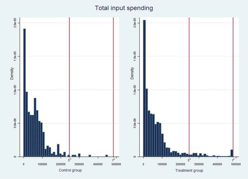
Figure 1 displays the distribution of the Total input spending variable in control and treatment groups. As may be noted, the treatment group clearly has more observations both near and beyond the threshold values. Thus, while extreme values obviously affect the exact results, it is also clear that the values for the Total input spending variable differ in general between the two groups, and that the results are not merely driven by a few outliers.

Figure 1. Distribution of values for the total input spending variable from the endline survey, indicating the 1% and 5% cut-off thresholds used in the robustness checks.

4.2. Choices of explanatory variables

An additional step in the robustness checks was to examine the effects of deselecting some explanatory variables. In the original paper, the authors reported that baseline variables from the first round of the survey were included in the regressions; however, the estimated coefficients for those variables were not reported in the paper or in the online appendices, making it difficult to judge how important the variables were for the outcomes. We examined this by dropping the entire H_ij vector from equations (1) and (2) and keeping only the stratification dummies S_j, instead estimating a modified set of equations, as follows:

(3) $Y_{ij}=\delta +\alpha Saving{s}_j+{{\beta }_S}^{\prime }{\mathit{S}}_j+{\epsilon }_{ij}$(3)

(4) $Y_{ij}=\delta +{\alpha }_{1}Ordinar{y}_j+{\alpha }_{2}Commitmen{t}_j+{{\beta }_S}^{\prime }{\mathit{S}}_j+{\epsilon }_{ij}$(4)

The results from these regressions are reported in Tables A.36 through A.39. The results are, once again, very similar to those in the original study. Most outcome variables that were statistically significant had larger coefficients and, occasionally, higher levels of statistical significance than their counterparts in the original study.

5. Theory-of-change analysis: effects for farmers who responded to the treatment

Although all farmers in the treatment groups were offered one of the bank account treatments, less than 20 per cent of those in the treatment groups responded to the treatment, in the sense that they actually opened and used one or more of the offered accounts. The standard approach in assessing the impact of a treatment like this is to examine the effect for the entire group that was offered the treatment. This is the approach the original authors took, and is what we did in Section 2 through 4.

However, it is presumably also of interest to policymakers to know what effect a policy has on those who make use of the opportunities that it offers, not merely what average effect offering a policy opportunity has on those who are eligible for it, whether they use it or not. We wish to point out, for instance, that a common approach in other agricultural extension activities is to ensure adoption by some farmers in the hope that early adopters’ success will gradually encourage others to follow suit. In our replication plan, we speculated that something similar could happen here: even if, relatively speaking, only a few farmers adopted the new savings vehicles at an early stage, if they had noticeable success with these vehicles, then that should encourage adoption by other farmers in the longer term. We therefore proposed exploring the outcomes for farmers that adopted the offered savings vehicles and made use of them.

Unlike the other parts of our replication study, this part was somewhat experimental and we explored a number of potential approaches, including propensity score matching (reported in more detail in Stage and Thangavelu 2018; the results reported there are similar in magnitude to those reported here). However, based on a useful suggestion from a reviewer, we finally settled on a simple approach that is minimalistic in terms of the assumptions necessary for the analysis to work. Since only farmers who were in the treatment group were able to open the offered accounts, we have one-sided non-compliance with a randomised treatment. Assuming that farmers who were in the treatment group but did not respond to the treatment were not affected by their assignment to the treatment group, the local average treatment effect is simply given by the average treatment effect divided by the share of compliers (see e.g. Imbens and Rubin 2015). The local average treatment effects, for the outcome variables of interest, are then as reported in Table 2.

Table 2. Local average treatment effects for farmers who opened and used bank accounts.

Variables
	Average value in the endline survey, all farmers	Local average treatment effect, compliers
Land under cultivation (acres)	4.52	1.55
Total value of inputs (MK)	68,046	41,356
Proceeds from crop sales (MK)	109,604	101,005
Value of crop output (sold and not sold) (MK)	177,747	123,304
Farm profit output (output – input) (MK)	110,703	87,253
Total expenditure in last 30 days (MK)	11,905	5,933

The estimated local average treatment effects are all positive, and are all substantial in magnitude compared to the sample averages. The estimated effect on proceeds from crop sales is almost as large as the average sales revenue for the sample as a whole; the effect on the average output value is almost 70% of the value for the sample as a whole; net profits increase by an amount corresponding to almost 80% of the sample average; and the effect on expenditure corresponds to almost 50% of the average value for the sample. All the estimated local average treatment effects suggest that, for the farmers who actually chose to make use of the offered bank accounts, the bank accounts were welfare improving.

While we think it is interesting to try to estimate outcomes for farmers who actually made use of the offered savings vehicles, there are a number of potential statistical issues that make this analysis less clear-cut than the analyses reported in Sections 2 through 4. As described in Section 1, all farmers in the treatment and the control groups were provided with general encouragement to save more for future input purchases. Thus, even farmers in the control group had characteristics that were slightly different from those of farmers in the general population.

There is also a possibility that farmers in the same club affected each other’s behaviour to some extent, even if they did not make the same choices about savings vehicles, so that observations of different farmers in the same club are not fully independent from a statistical standpoint. Thus, for instance, a farmer who chose not to open a savings account might nonetheless see neighbours who did subsequently spending more on inputs, and choose to emulate that behaviour (in which case the exclusion restriction would not hold). To the extent that these types of effects mattered, it seems likely that they would reduce the estimated impact of opening and using the savings accounts, so the fact that these impacts were nonetheless estimated to be so large is, we believe, interesting. Nonetheless, these cautions need to be borne in mind.

6. Concluding remarks

Brune and colleagues (2016) research is an important contribution to the academic literature on the impact of microfinance. Although we hope our replication study also contributes to this literature, we would like to stress that the replication work was not occasioned by any misgivings on our part about the original research; rather, we were interested in the original study and hoped to enhance its relevance to policymakers and future researchers.

We only had access to data that had already been cleaned and winsorised. However, with that caveat, our results were generally supportive of the original study. All results from our push-button and pure replications are consistent with the results reported by the original authors; the few minor discrepancies we found do not affect the conclusions drawn in their paper.

The results from our estimation analysis are also generally in support of the findings in the original paper. In some cases, these checks led to lower statistical significance and/or smaller estimated coefficients than in the original study, while in other cases, they led to higher statistical significance and/or larger coefficients. Nonetheless, these checks did not reveal any systematic problems with the original analysis.

Moreover, in our examination of farmers who had chosen to make use of the offered financial products – an extension the original authors did not make in their study – our results also indicate support for the findings from the original study. Adopting the offered savings vehicle led to substantial increases in farm output and profits. The timeframe studied in the experiment was relatively short, and adoption of the savings vehicles was fairly limited during this time. However, considering the large effects for farmers who did adopt the savings vehicles, it does not seem unreasonable that neighbours who observed this would also begin to adopt the treatment, and that, in future, its positive effects could grow even beyond those reported in the original study.

It is clear that more research is needed to identify the causal mechanisms through which improved access to savings vehicles led to improved farming outcomes and improved well-being among the targeted farmers. Notably, in similar future experiments, it would probably be useful to include survey questions probing farmers’ access to different social networks that provide informal mechanisms for savings and borrowing. Qualitative in-depth interviews with some of the participating farmers could help explore their motives for making use of the vehicles or not. We also believe a larger control group would have made it easier to evaluate some of the effects studied, both for our study and for the original authors, and recommend that future experiments on similar topics ensure a sufficiently large control group.

Nonetheless, even if the exact mechanisms remain to be investigated, it is obvious that farming outcomes and well-being were improved by this intervention. Thus, we would make recommendations similar to those of the original authors. Offering these savings vehicles to more farmers would thus be good agricultural policy.

Acknowledgments

We are grateful to the International Initiative for Impact Evaluation (3ie) for funding and for technical review and support throughout this study under the 3ie Replication Programme. Our deep gratitude also goes to Lasse Brune, Xavier Giné, Jessica Goldberg and Dean Yang for providing the data and code from their original paper. Finally, we thank 3ie’s internal and external reviewers for their valuable input to our replication plans and the journal’s reviewer for constructive comments on the journal version of the paper.

Disclosure statement

No potential conflict of interest was reported by the authors.

Supplementary material

Supplemental data for this article can be accessed here

Additional information

Funding

This work was supported by the International Initiative for Impact Evaluation.

Notes on contributors

Jesper Stage

Jesper Stage is a professor of economics at Luleå University of Technology in Sweden. He has worked on agricultural,environmental and natural resource economics in developing countries for over twenty years.

Tharshini Thangavelu

Tharshini Thangavelu is currently a post doctoral researcher at Karolinska Institutet in Sweden. She has a PhD from LuleåUniversity of Technology in Sweden. Her research is in health, environmental and development economics.

Notes

1. In a survey of studies on financial literacy, Miller and colleagues (2014) found that financial literacy training was usually found to improve savings rates. Although the financial training provided as part of this experiment was relatively limited, even the farmers in the control group were likely to have begun saving more than farmers who were not part of the experiment at all.

References

- Akerlof, G. A. 1970. “The Market for ‘lemons’: Quality Uncertainty and the Market Mechanism.” Quarterly Journal of Economics 84 (3): 488–500. doi:10.2307/1879431.
- Anderson, S., and J.-M. Baland. 2002. “The Economics of ROSCAs and Intrahousehold Resource Allocation.” Quarterly Journal of Economics 117 (3): 963–995. doi:10.1162/003355302760193931.
- Andersson, C., E. Holmgren, J. MacGregor, and J. Stage. 2011. “Formal Microlending and Adverse (or Non-existent) Selection: A Case Study of Shrimp Farmers in Bangladesh.” Applied Economics 43 (28): 4203–4211. doi:10.1080/00036846.2010.491444.
- Armendáriz, B., and J. Morduch. 2005. The Economics of Microfinance. Cambridge: MIT Press.
- Ashraf, N., D. Karlan, and W. Yin. 2006. “Tying Odysseus to the Mast: Evidence from a Commitment Savings Product in the Philippines.” Quarterly Journal of Economics 121 (2): 635–672. doi:10.1162/qjec.2006.121.2.635.
- Brown, A. N., D. B. Cameron, and B. D. K. Wood. 2014. “Quality Evidence for Policymaking: I’ll Believe It When I See the Replication.” Journal of Development Effectiveness 6 (3): 215–235. doi:10.1080/19439342.2014.944555.
- Brune, L., X. Giné, J. Goldberg, and D. Yang. 2016. “Facilitating Savings for Agriculture: Field Experimental Evidence from Malawi.” Economic Development and Cultural Change 64 (2): 187–220. doi:10.1086/684014.
- CGAP and IFC. 2013. Financial Inclusion Targets and Goals: Landscape and GPFI View. Washington, DC: Consultative Group to Assist the Poor (CGAP) and International Finance Corporation (IFC).
- Deaton, A. 1989. “Saving in Developing Countries: Theory and Review.” World Bank Economic Review 3 (S1): 61–96. doi:10.1093/wber/3.suppl_1.61.
- Dercon, S. 2002. “Income Risk, Coping Strategies, and Safety Nets.” World Bank Research Observer 17 (2): 141–166. doi:10.1093/wbro/17.2.141.
- Dixon, W. J. 1960. “Simplified Estimation from Censored Normal Samples.” Annals of Mathematical Statistics 31 (2): 385–391. doi:10.1214/aoms/1177705900.
- Dupas, P., D. Karlan, J. Robinson, and D. Ubfal. 2018. “Banking the Unbanked? Evidence from Three Countries.” American Economic Journal 10 (2): 257–297.
- Duvendack, M., R. Palmer-Jones, J. G. Copestake, L. Hooper, Y. Loke, and N. Rao, 2011. “What Is the Evidence of the Impact of Microfinance on the Well-being of Poor People?” EPPI-Centre, Social Science Research Unit, Institute of Education, University of London.
- Giné, X., J. Goldberg, and D. Yang. 2012. “Credit Market Consequences of Improved Personal Identification: Field Experimental Evidence from Malawi.” American Economic Review 102 (6): 2923–2954. doi:10.1257/aer.102.6.2923.
- Gugerty, M. K. 2007. “You Can’t Save Alone: Commitment in Rotating Savings and Credit Associations in Kenya.” Economic Development and Cultural Change 55 (2): 251–282. doi:10.1086/508716.
- Hermes, N., and R. Lensink. 2007. “The Empirics of Microfinance: What Do We Know?” Economic Journal 117 (517): F1–10. doi:10.1111/j.1468-0297.2007.02013.x.
- Hoff, K., and J. E. Stiglitz. 1993. “Imperfect Information and Rural Credit Markets: Puzzles and Policy Perspectives.” In The Economics of Rural Organization: Theory, Practice, and Policy, edited by K. Hoff, A. Braverman, and J. E. Stiglitz, 33–52. New York: Oxford University Press.
- Imbens, G. W., and D. B. Rubin. 2015. Causal Inference for Statistics, Social, and Biomedical Sciences: An Introduction. Cambridge: Cambridge University Press.
- Miller, M., J. Reichelstein, C. Salas, and B. Zia 2014. Can You Help Someone Become Financially Capable? A Meta-analysis of the Literature. World Bank Policy Research Working Paper 6745, Washington, DC: World Bank.
- Platteau, J.-P. 2000. Institutions, Social Norms, and Economics Development. Amsterdam: Harwood.
- Prina, S. 2015. “Banking the Poor via Savings Accounts: Evidence from a Field Experiment.” Journal of Development Economics 115 (1): 16–31. doi:10.1016/j.jdeveco.2015.01.004.
- Robinson, M. 2001. The Microfinance Revolution: Sustainable Finance for the Poor. Washington, DC: World Bank.
- Rutherford, S. 2000. The Poor and Their Money. Oxford: Oxford University Press.
- Selander, C., J. Stage, J. Stage, and J. Öberg. 2006. “The Impacts of Microcredits – A Case Study from Kenyan Agriculture.” Journal of Development Alternatives and Area Studies 25 (1–2): 5–20.
- Stage, J., and T. Thangavelu. 2017. Revisiting Savings: A Replication Study of Facilitating Savings for Agriculture. Replication Plan. Washington, DC: International Initiative for Impact Evaluation (3ie). https://www.3ieimpact.org/sites/default/files/2018-12/stage_revised_replication_plan.pdf
- Stage, J., and T. Thangavelu, 2018. Savings Revisited. A Replication Study of A Savings Intervention in Malawi. 3ie Replication paper 18, Washington, DC: International Initiative for Impact Evaluation (3ie). https://www.3ieimpact.org/evidence-hub/publications/replication-papers/savings-revisited-replication-study-savings#3001
- Stewart, R., C. van Rooyen, M. Korth, A. Chereni, N. Rebelo Da Silva, and T. de Wet. 2012. Do Micro-credit, Micro-savings and Micro-leasing Serve as Effective Financial Inclusion Interventions Enabling Poor People, and Especially Women, to Engage in Meaningful Economic Opportunities in Low- and Middle-income Countries? A Systematic Review of the Evidence. EPPI-Centre, Social Science Research Unit, Institute of Education, University of London.
- Stiglitz, J. E., and A. Weiss. 1981. “Credit Rationing in Markets with Imperfect Information.” American Economic Review 71 (3): 393–410.
- Thangavelu, T., and J. Stage. 2018. Replication Data For: Savings Revisited. A Replication Study of Savings Intervention in Malawi. Harvard Dataverse, V1. doi:10.7910/DVN/PBALME.