Finite elements-based 2D theoretical analysis of the effect of IEX membrane thickness and salt solution residence time on the ion transport within a salinity gradient power reverse electrodialysis half cell pair

Abstract

Reverse electrodialysis electrical power generation is based on the transport of salt ions through ion conductive membranes. The ion flux, equivalent to an electric current, results from a salinity gradient, induced by two salt solutions at significantly different concentrations. Such equivalent electric current in combination with the corresponding electrochemical potential difference across the membrane, equivalent to an electric potential, results in a battery equivalency. While having a co-current fluid flow of both solutions in the reverse electrodialysis cell pair compartments, a mathematical model needs to be based on both diffusion and convective mass transport equations in the compartments and on the, electromigration-based, ion transport through the membranes. The steady state salt ion flux through the membranes and the corresponding ion concentration distribution within the salt solution compartments of a reverse electrodialysis cell pair (in the absence of electrodes) was theoretically analysed by using two-dimensional finite element (FEM) modelling. Fundamental information on the effect of membrane thickness and fluid flow velocity was obtained. FEM simulations support the theoretical insight into reverse electrodialysis phenomena and thus assist in the planning/design of experimental work. The FEM approximation is superior with respect to a modelling of the combined effect of all complex and simultaneous ion transport mechanisms in the reverse electrodialysis cell pair compartments and ion conductive membranes. In fact, this first time reporting of a FEM modelling of a half cell pair obviously also includes the complex and dynamic drop in salinity gradient, between influent side and effluent side, over the height of the half cell pair compartments.

Keywords:

• Salinity gradient
• Reverse electrodialysis
• Finite element
• Power
• Model
• Steady state
• Flow
• Concentration distribution
• Diffusion
• Electromigration

1. Introduction

The energy production potential, from the mixing of two salt solutions showing a large concentration difference (Salinity Gradient; SG), has recently gained significant attention. The potential of harvesting osmotic energy was already indicated early in scientific literature [1–4]1234. The interest in osmotic energy revived at the end of last century [5,6]56. Two main technical approaches exist: reverse electrodialysis (Fig. 1) or pressure retarded osmosis (PRO). PRO is under detailed investigation by e.g. Statkraft in Norway [7].

Fig. 1 Principle of a complete SGP-RE battery.

Reverse electrodialysis can be based on the mixing of fresh water (river and lake) and seawater, being typically called “Blue Energy” (RED) [8–15]89101112131415 but also on the mixing of highly concentrated brine with seawater/brackish water (called SGP-RE to make the distinction) [16–20]1617181920. In the case of RED, the seawater/fresh water SG is indeed typically 30–35 kg/m³ whereas, in the case of SGP-RE, the SG can be nearly 10 times higher, thus typically 270–300 kg/m³. When compared to RED, such a high SG in the case of SGP-RE should enable to induce an importantly higher salinity gradient power (SGP) output in a reverse electrodialysis stack, when expressed as W/m² cell pair [3] or as kW/m³ stack [Table 2 in 17].

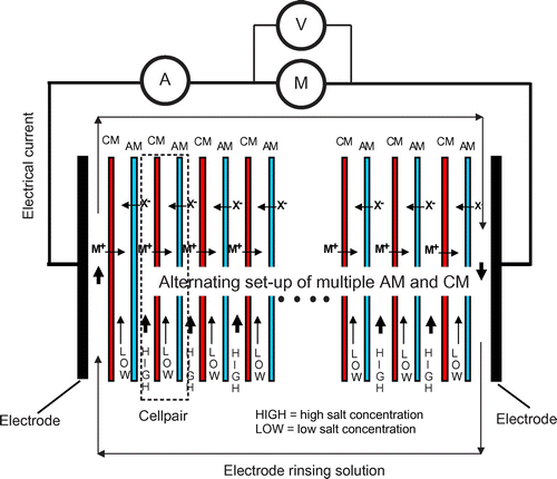
It is clear that a mathematical modelling of the SGP-RE phenomena on the basis of a cell pair (Fig. 1) assists in acquiring insight regarding the importance of specific SGP-RE process parameters. The model approach by Lacey as reported in [3,17]317 is a “simplified” modelling approach considering the total resistance of the membrane/compartments of the cell pair (basic unity building block of a SGP-RE battery; Fig. 2). The approach indeed needs to be looked upon as idealised since e.g. describing a cell pair without taking into account the important drop in SG (salinity gradient) between the stack influent side and the stack effluent side in a real SGP-RE stack, as a result of the ion transport through the membranes from the HIGH compartment towards the LOW compartment. In fact, the Lacey model could be considered as a “1-D” cell pair model in that respect.

Fig. 2 Basic SGP-RE cell pair [17].

An obvious step forward towards a more refined FEM model was lacking. As a result, such first time FEM model simulation was performed and is introduced in this publication. Specifically for the SGP-RE case a two-dimensional(2D) FEM basic simulation was studied on the basis of two NaCl model solutions of, respectively, 0.6 M (“seawater” concentration type; called LOW) and 4.5 M (concentrated brine concentration type; called HIGH). When compared to the approach by Lacey [3,17]317, a FEM-based simulation needs to be considered as a highly sophisticated modelling approximation of the complex real phenomena within a basic cell pair as illustrated in Fig. 1.

Moreover, in the compartments of a cell pair in a real SGP-RE battery stack, spacers are present which influence, in a complex way, the fluid dynamics and convection-diffusion phenomena within those compartments (laminar mixing in the compartments). A co-current fluid flow of both solutions in the reverse electrodialysis cell pair compartments is assumed here. The electromigration-based ion transport of the ions through the membranes needed to be implemented in the model as well. The extremely complex dynamics of such simultaneously ongoing transport phenomena in the cell pair compartments and membranes can only be described in detail and to a good approximation through the introduction of appropriate differential equations describing the convection–diffusion and electromigration phenomena. The steady-state salt ion transport through the membranes and the corresponding ion concentration distribution within the salt solution compartments of a reverse electrodialysis cell pair (in the absence of electrodes) could be theoretically and successfully analysed. In particular, the important effect of the membrane thickness and the salt solution flow velocity was investigated and highlighted.

2 Simulation methods

2.1 Introduction

The SGP-RE process is linked to the conversion of the available mixing energy of a HIGH and a LOW salt solution. In that respect, an ion conductive membrane within a cell pair can be considered as the crucial location where the electrochemical conversion of the mixing energy is realised. Across the membrane, a difference in electrochemical potential between HIGH and LOW exist. This can be viewed upon as the creation of an electrical potential across the membrane. The transport of the ions through the membrane is also equivalent to an electric current. As a result, the combination of the electrical potential and the electrical current enables to drain electrical power from the cell pair. In principle the fundamental information, related to the energy production through SGP-RE, thus can be confined to the theoretical modelling of the phenomena within a single cell pair.

All other SGP-RE related “practical” aspects related to the total description and modelling of a full SGP-RE stack, including the:

1. combined electrochemical action of N cell pairs in series

2. phenomena linked to the SGP-RE stack electrodes and electrode rinsing solution

3. electrical interaction with an actual electrical load, connected to the electrodes

4. pumping energy requirements linked to the transport of the HIGH and LOW solutions through their respective compartments

are not considered in this publication. The verification of a full SGP-RE stack model including the items A-D on the basis of experimental data obtained from a real stack is not the subject of this publication. In that respect, project Work Package 5 within the REAPower (http://www.reapower.eu) project will deliver more detailed information while being based on the full SGP-RE stack approach, including the items A-D. The publication of such information will be performed in the future by the University of Palermo.

The FEM-based theoretical modelling is thus confined in this publication to the description of the electrochemical activity and power production on the basis of a cell pair (in the absence of electrodes). In that respect, it should be remarked first that in the modelling by Lacey [3] and in [17] a cell pair, as illustrated in Fig. 2, was used. The representation within Fig. 2 and the approach in [3,17]317 describe, in a simplified way, the basic transport of anions and cations within a cell pair from the highly concentrated salt solution compartment (HIGH) into the low concentration salt solution compartment (LOW) on an “electrical resistance” basis. Moreover, the concentration profile within a boundary layer δ at the membrane surface was approximated in a simplified, linear way. In Fig. 2, the bulk concentration N_LOW in the LOW compartment is thus assumed to increase linearly towards the values N1 and N4. The corresponding drop within the HIGH compartment from the bulk value N_HIGH was also approximated in a linear way towards the values N5 and N8.

In practice such diffusion driven ion concentration profiles within the respective compartments at the boundary locations (diffusion boundary layer) are evidently non-linear or discontinuous in locations 2, 3, 6 and 7 in Fig. 2. Also the assumption in the approach of Fig. 2 was made that the concentration distribution is the same over the cell pair height (“1-D” approach). Therefore, a sophisticated FEM approach was introduced to highly exceed the restricted model approach within [3,17]317 and of which the simulation methods and results will be discussed in the next sections.

2.2 Half cell pair FEM geometry approach

The diffusion related boundary layer concentration profiles in Fig. 2 within the HIGH compartment will show in reality, a continuously decreasing concentration towards the membrane surface from the bulk in the middle of the HIGH compartment. When introducing a FEM-based simulation such continuous boundary layer concentration and diffusion profile will be simulated automatically. In an analogous way, this is also the case for the continuously increasing concentration towards the membrane surface in the boundary layer within the LOW compartment. As well, FEM simulations will thus also not show the type of discontinuities as represented within locations 2 and 3 as depicted in Fig. 2.

It will be shown first that the basic geometry needed in a FEM approach to model the phenomena at the level of a SGP-RE cell pair can be reduced to the restricted set-up depicted within Fig. 3(b) and even beyond that (see 2.5).

Fig. 3 Representation (2D) of membrane, HIGH and LOW compartments.

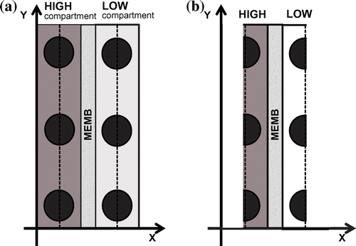
As indicated in Fig. 1, each cell pair consists of a HIGH compartment, an AM, a LOW compartment and a CM. In those cell pairs, there is a simultaneous transport of anions (through the AM) and cations (through the CM) in opposite directions, thereby assuring a steady state and an overall electrical neutrality regarding the presence of anions and cations in the HIGH and LOW compartments. Therefore, in steady state, the charge amount of anions (on a total electrical charge basis) being transported through the AM from a HIGH compartment to a neighbouring LOW compartment should be in equilibrium with the charge amount of cations (on a total electrical charge basis) being transported through the CM into the same LOW compartment from a second neighbouring HIGH compartment. As a result, the reader needs to allow here, for simulation reasons, the implementation of an important abstraction which largely increases the efficiency of the FEM modelling while preserving fundamental information about the ion transport phenomena.

In an actual SGP-RE battery cell pair, one of both membranes will show the smallest ion transport rate and thus will dictate the overall ion transport rate. It is thus very convenient to make an important abstraction while reducing the modelling towards one single (slowest) representative ion “X” linked to the rate dictating membrane (whatever AM or CM dictating that transport rate). That ion “X” is moreover assumed in this publication to have an ion valence of 1. The constituent X thus represents, in an abstract way, both an anion (Cl⁻) and a cation (Na⁺). From this Na⁺ and Cl⁻ ions, transport rate equilibrium in steady state in a cell pair is possible to introduce the set-up as presented in Fig. 3(a), while introducing spacers in the HIGH and LOW compartments. A spacer was approximated in the 2D approach by solid circles. The HIGH and LOW compartment geometries within Fig. 3(a) in fact also show an axial symmetry at their centres (represented by the dotted lines). As a result, a further convenient abstraction and geometry reduction can be made since the ion transport is also dictated by these symmetry centre lines. In principle, a 2D FEM simulation of the SGP-RE phenomena then can be based on the geometry as represented in Fig. 3(b). The geometry represented in Fig. 3(b) is called in this publication a “half cell pair”.

2.3 Ion transport within the membrane in the half cell pair

The ion conductive membrane material within Fig. 3(b) is assumed to be perfectly homogeneous, thus showing a constant IEC (ion exchange capacity) over its total bulk (typically 1,500 mol/m³). A valence z = 1 is assumed here for the fixed ions as well as for the anions and cations in the HIGH and LOW salt solutions (e.g. NaCl solutions). For electroneutrality each fixed ion then needs to be compensated by a counter-ion. Therefore, the concentration of counter-ions is considered to be homogeneous in the membrane. In the case of one type of cation (Na⁺) and one type of anion (Cl⁻) as counter-ions, it is thus assumed that in the cation conductive membrane the Na⁺ ions are homogeneously distributed over the CM bulk. There is then no Na⁺ concentration gradient within the CM itself (the concentration profile is flat/horizontal). A Na⁺ ion entering the membrane at the HIGH-membrane interface thus causes one Na⁺ ion to move into the LOW compartment at the LOW-membrane interface. This transport is only possible through multiple simultaneous hopping events of Na⁺ counter-ions from one fixed anion location to a neighbouring fixed ion location in the x-direction. The same reasoning can be implemented for the Cl⁻ ion in the AM.

With respect to the ion transport phenomena in the membrane, a reference can be made first in general to the Nernst-Planck equation which describes an ion flux J in a medium while being generated from the combined action of a concentration gradient [dc/dx; left part of Eq. (1)] and the electromigration in an electric field [dE/dx; right part of Eq. (1)]. Regarding the representation of the flux J in its modulus format |J| in this publication the reader is referred to the analogous discussion below, on the use of the modulus format when expressing |ΔE| (thus avoiding possible confusion related to technical sign conventions in technical electrical circuitry presentation). Obviously, the flux in Fig. 3(b) is from the HIGH compartment to the LOW compartment, thus from left to right.(1)

J = flux [mol/(m² s)], D = diffusion coefficient [m/s²], c = concentration [mol/m³], F = Faraday [96485.34 C/mol], z = valence, R = gas constant [8.3144621 J/(mol K)], T = temperature [K].

As already explained, it is assumed that an ion conductive membrane shows a homogeneous distribution, thus homogeneous concentration, of the single counter-ion (Na⁺ or Cl⁻ since it is assumed that there are no other ions present in the simulation considered in this publication) over its bulk. There is then no concentration gradient inside the membrane (thus a flat concentration profile causing dc/dx = 0; concentration value is typical 1,500 mol/m³). Therefore, regarding the ion transport within the membrane, only the second part of Eq. (1) is then relevant:(2)

At the interface location “A” between the HIGH solution and the membrane, there is a higher concentration of X when compared to the interface location “B” between the membrane and the LOW solution. Therefore, there is a difference in electrochemical potential between interface locations “A” and “B”. It is then possible to introduce here the potential drop |ΔE| = f(y) across the membrane as derived by Strathmann [20]; [Eq. (2).184 p. 84]:(3) t_m,cou = transport number of the counterion in the membrane, t_m,co = transport number of the co-ion in the membrane, a_X,HIGH = activity of X in the HIGH solution, a_X,LOW = activity of X in the LOW solution, α = membrane permselectivity.

Regarding Eq. (3) Strathmann indicates in [21]: “To a first approximation the membrane potential is identical to the measured membrane potential”.

The potential |ΔE| within Eq. (3) is indicated here in its modulus format in order to avoid discussions on the specific sign conventions (as introduced and agreed upon during the history of the theory on electricity). Such sign conventions indeed could blur the discussion with respect to the interpretation of the flux as expressed by Eq. (1). At the level of a half cell pair, as depicted in Fig. 3(b), it is however very obvious that the ions X will move from the HIGH compartment through the membrane towards the LOW compartment. That transport can be considered to be driven as an electromigration driven transport since the potential drop |ΔE| = f(y) over the membrane creates an electrical field in the membrane. When assuming a homogeneous electrical field in the x-direction across the membrane thickness (of course at the influent location y = 0 the electrical field is larger than at the effluent location y = H at the top of the compartments), the value of the electric field (V/m) is assumed to be well approximated by(4)

After the implementation of Eq. (4), Eq. (2) then results in:(5)

D_memb = diffusion/(electromigration) coefficient of X in the IEX membrane [m/s²], c_memb = IEC of the IEX membrane [typically 1,500 mol/m³], z = valence (assumed to be 1 in this publication), W_memb = membrane thickness (m).

Eq. (3) can be introduced in Eq. (5) resulting in:(6)

It is also trivial that J as a flux [mol/(m² s)] represents the movement of ions, thus J also represents (when multiplying its value by the Faraday constant [C/mol]) an electric current density [A/m²]. Since only a half cell pair is considered in this publication, an abstraction towards the ion X representing both the anion and cation is possible.

The reader should notice here that if (s)he intends to model a full cell pair (see item A in 2.1), it will be needed to consider two half cell pairs with:

1. an anion conductive membrane taking care of the transport of the anions. The direction of the J_anion flux vector will be opposite to the direction of the electrical current density vector (based on the electrical abstract convention that the “electrical current” vector direction involves the transport direction of positively charged particles). In an analogous way, the “electrical potential“ sign/profile across the membrane will be opposite to the electrochemical potential profile across the membrane

2. a cation conductive membrane taking care of the transport of the cations. Now the direction of the J_anion flux vector will be the same as the direction of the electrical current density vector. In this case, the electrical potential profile across the membrane will be congruent to the electrochemical potential profile across the membrane

It is also important to note that, in principle, Eq. (6) could be converted to a “lower technical” level of a “resistance” based on ΔE = R.I thereby combining within Eq. (6) the D_memb and c_memb values as to obtain an equation holding the “resistance” value. By doing so, phenomena details related to the mobility of the ions within the membrane matrix and the concentration of the ions within the membrane are simply lost. In such a way, important phenomena linked information are also lost in the modelling and specifically in the Comsol Multiphysics (CMP) FEM simulations described within this publication, the approach of Eq. (6) at a “higher level” is therefore definitely preferred over a “resistance” approach.

2.4 Ion transport and fluid dynamics within the compartments of the half cell pair

The fluid flow of the HIGH and LOW solutions in their respective compartments is laminar at the low velocities, as used in practice (e.g. 1 cm/s). Nevertheless, the presence of a spacer enhances the convective transport of ions towards the membrane surface (“laminar mixing”).

In CMP, the steady state fluid flow situation can be simulated. The fluid flow in the HIGH and LOW compartments was set to single-phase laminar flow. The Eqs. (7,8), available within CMP [22] and relevant to such single-phase laminar flow, are based on the Navier–Stokes approach for incompressible flow of both the HIGH and LOW solutions.(7) (8)

The term at the left in (7), related to “ρ”, represents inertia. The term related to “p” represents the pressure gradient. The term related to “μ” represents viscosity, while Force represents “other” body forces (e.g. gravity or, when relevant, also centrifugal forces). Eq. (8) represents the conservation of volume in the case of incompressibility.

In the HIGH and LOW compartments, the ruling transport equation for the convection–diffusion transport is (as used by CMP [22]):(9)

Eq. (9) clearly involves the concentration gradient determined by ion transport in the HIGH and LOW salt solution-based domains. This is in contrast with the transport mechanism in the membrane which is electromigration, as explained in 2.3.

2.5 Boundary conditions in the half cell pair

When limiting to a model describing the steady state within a half cell pair, it is thus interesting to note, when accepting all preceding assumptions, that in steady state the flux of ion X through the ion conductive membrane can be approximated by Eq. (6), thus using the activity a_X,HIGH = f(y) at the HIGH/membrane interface and using the activity a_X,LOW = f(y) at the LOW/membrane interface. When further assuming a constant value of D_memb value across the membrane and considering the steady state, the value of the flux J(y) evidently has the same value in both interfaces. Such can then be used to express a boundary condition in the FEM model. It is trivial that the implementation within the CMP FEM environment of the ion X flux at the boundaries of the domains (HIGH and LOW domains) requires correct CMP software prescribed sign conventions (a flux going out of a domain is negative; a flux going into a domain is positive).

From all previous points of view with respect to the implementation of the Eq. (6) based boundary condition, it is now even possible to make the additional assumption that in the 2D FEM model a membrane domain is in fact not explicitly needed. Eq. (6) can be put as an algebraic equation regarding the boundary condition at the boundary interface between the HIGH and the membrane and as a boundary condition at the boundary interface between the LOW and the membrane. The membrane can indeed be assumed under the conditions of a single salt (NaCl) as merely a convenient transport medium showing the same flux profile over each vertical section within the membrane thickness related Δx-interval. It is thus even feasible to omit the membrane domain in the 2D model altogether and, in an abstract way, combine both boundaries into one single boundary fully dictated by Eq. (6). This approach was used in the simulations within this publication. In the 2D approach only half of one cell pair was thus modelled according to Fig. 3(b) while replacing the MEMB domain of Fig. 3(b) by one single boundary. It should be noted that future FEM modelling of entire and multiple cell pairs of course still could be based on the algebraic approach of Eq. (6) while including a symbolical “membrane domain” when geometrically needed (and the two boundaries HIGH/MEMB and MEMB/LOW), using the method of the projection (over the symbolical membrane geometrical domain) of the flux boundary condition (Eq. (6)) from the HIGH/MEMB boundary onto the MEMB/LOW boundary.

The domains HIGH and LOW as illustrated in Fig. 4 were implemented in CMP. Boundary conditions with respect to concentration, flux and flow were defined for all boundaries. At the HIGH and LOW domain entrance boundaries, the concentrations of the HIGH and LOW influent have, respectively, the values 4,500 and 600 mol/m³. The effluent boundaries of the HIGH and LOW domains were defined in CMP as Outflow boundaries showing a zero relative pressure outlet. The dotted line boundaries in Fig. 3(b) are considered to be of the No Flux type. In CMP, the domains HIGH and LOW have, respectively, the domain labels 1 and 2. Concentrations in the HIGH and LOW domains are then, respectively, c1 and c2, combined in an overall total domain concentration cALL (cALL = c1 in the HIGH domain; cALL = c2 in the LOW domain). As already indicated, the “combined” boundary between the HIGH and LOW domains, are based on the condition specified algebraically by Eq. (6).

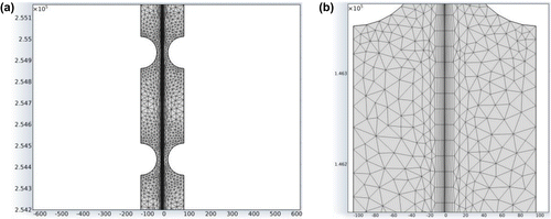
Fig. 4 FEM geometry and meshing as used in the simulations.

2.6 FEM meshing approach of the half cell pair

The FEM model as used in the simulations within this publication was based on the geometry/meshing as illustrated in Fig. 4(a) and (b) (B as a detail of the domains HIGH at the left and LOW at the right having a single boundary, as explained in 2.3, between them). The coordinate units within Fig. 4 are in micrometres for both the x- and y-axis (y-axis: times 100 000 as indicated in the upper left corner of the graphs).

In the simulations, the height H_memb of the half cell pair was set to 0.256 m while the full HIGH and LOW compartment widths in Fig. 3(a) were both 2 E-6 m. The width of the model domains HIGH and LOW in Fig. 3(b) and Fig. 4 was 1 E-6 m for each domain (half of the full HIGH and LOW compartments). Evidently, the ratio H_memb versus the small HIGH and LOW compartments width is very large. The geometrical construction of the domains HIGH and LOW was performed on the basis of a single basic geometrical unit of 0.5 E-3 m in height, including one spacer wire. This basic geometrical unit (height 0.5 mm) was doubled and combined in one new geometrical element (1 mm height). Repeating this doubling strategy resulted in an exponentially increasing total element height in a series of 2, 4, 8, 16, … , 128 mm until the final 256 mm total domain height (thus 512 basic geometrical units in total over the half cell pair height). The HIGH geometry within Fig. 3(b) is thus extremely thin (100 μm) when compared to its total height (256,000 μm). In CMP version 4.3a, such long and thin structure however could be successfully meshed and calculated for when using the MUMPS solver.

As a result of the need for a more detailed calculation at the boundary between HIGH and LOW, a boundary layer mesh was introduced at that boundary, as can be observed in Fig. 4(b) in more detail. This guarantees (a needed) much higher calculated data resolution in the immediate vicinity of the interface (in fact the membrane is represented in an abstract way by this mutual boundary) between the HIGH and the LOW domains.

3 Material characteristics used in the simulations

3.1 HIGH and LOW salt solution characteristics

3.1.1 Viscosity and density in the HIGH and LOW domains

Since the HIGH and LOW ion concentration values are high in this study, the implementation within the CMP FEM modelling of the dependence of the fluid dynamics on fluid viscosity and fluid density upon the concentration was considered to be essential. Indeed during the transport of the HIGH from the influent location y = 0 to the effluent location y = stack height, the concentration evidently will decrease as a result of the ion transport out of the HIGH domain. Moreover, the final steady state convective–diffusive transport gives rise to a concentration distribution in both the y and x direction within the HIGH and LOW domains. Moreover, the presence of the spacer has a profound effect on the fluid velocity field within the compartments. The spatial dependency regarding density and viscosity determines also the fluid flow behaviour and laminar velocity profile in both compartments. In this study, the assumption was made that the HIGH and LOW salt solutions were NaCl solutions, in order to be able to implement viscosity = f(c,T) and density = f(c,T) concentration and temperature dependencies.

Viscosity data in the temperature range of 10–40°C were extracted from [23] and processed by a well-fitting second-degree polynomial regression:(10)

The regression coefficient R² showed a typical value of R² = 0.9994 indicating a very good regression. The polynomial regression coefficients a₁, a₂ and a₃ are temperature depending. Those coefficients a_i(T) (i = 1,2,3) could also be well modelled through a second-degree polynomial regression approach of the format:(11)

Density data in the temperature range of 0–50°C were extracted from [24] and processed in an analogous way through second-degree polynomial regression as in the case of the viscosity. The same equation format as presented by Eqs. (10) and (11) was used since there is an analogous temperature dependency of the regression coefficients of type a_i(T). Regression coefficient R² showed also a typical value of R² = 0.9998 which also indicates a very good regression for fluid density.

In CMP, it is possible to put a complete expression for any material characteristic in the Variables dialogue window under Equation View. This was performed for viscosity and density. In this way, it is assured that the CMP FEM model will generate an even more realistic FEM calculated fluid flow dynamics/distribution in the compartments HIGH and LOW.

3.1.2 Diffusion coefficient in the HIGH and LOW domains

In [25 (← Figure 3)], experimentally determined diffusion data for NaCl solutions are presented. On the basis of that information, a diffusion coefficient value of D = 1.0E-9 m²/s was assumed in the CMP simulations. The simulation results in this publication are considered to be informative as a first approximation. A refinement towards the D(c,T) effects of temperature and concentration could be introduced in the future.

3.2 Membrane diffusion coefficient

Experimental data on the diffusion coefficients of ions within typical ion conductive membranes are reported in [14,26,27]142627. From these data, it can be concluded that the diffusion coefficient value is situated in the typical range of D_memb = 5E-11 m²/s to D_memb = 20E-11 m²/s. A value of D_memb = 5E-11 m²/s for the ion X was thus assumed here in the simulations. Nonetheless, it is obvious that membranes which exist show a higher diffusion coefficient value. It is then assumed here that the simulation results on the basis of D_memb = 5E-11 m²/s could be considered as “conservative”. It should be remarked that no sensitivity analysis was targeted with respect to the effect of the value of the diffusion coefficient linked to the membrane material. The simulation results on the basis of one well-chosen single value of D_memb are presented in Figs. 5–105678910 are considered to provide sufficient and important first quantitative information on the very complex phenomena in a half cell pair.

Fig. 5 Velocity profile in the HIGH and LOW compartments.

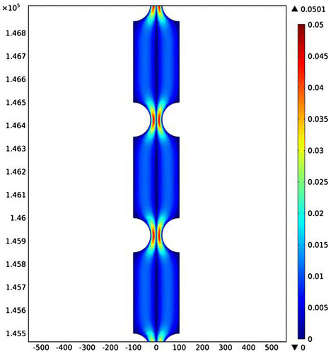
Fig. 6 Horizontal concentration cuts in the Vel2 case for different membrane thicknesses.

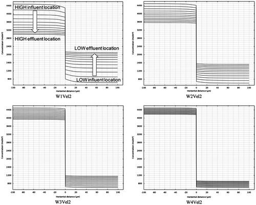
Fig. 7 Concentration profiles for W1 (left) and W4 (right).

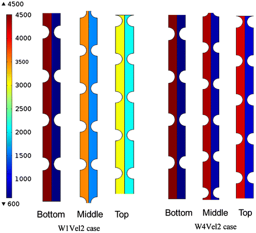
Fig. 8 Effect of membrane thickness (W1-W4) linked to the Vel2 condition.

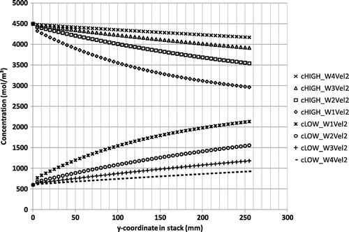
Fig. 9 Effect of membrane thickness & fluid velocity on ion X transfer rate.

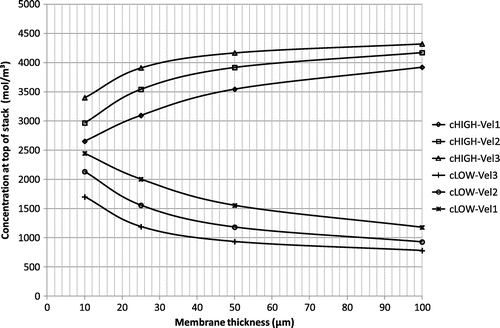
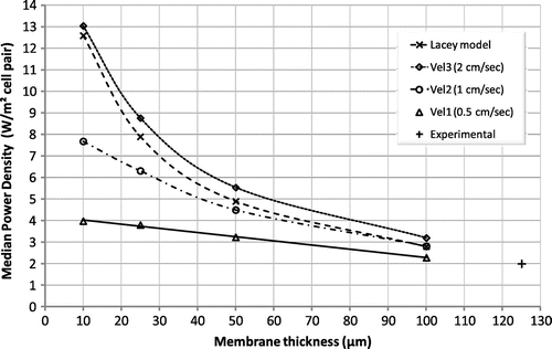
Fig. 10 Effect of membrane thickness & fluid velocity on half cell pair power density.

Since data on the temperature dependence of diffusion coefficients were not available at the time of the simulations it should be noted that a more detailed simulation exercise could be performed in the future.

4 FEM simulation results and discussion

4.1 Basic approach and FEM simulation parameter values

The importance of the membrane thickness is obvious from Eq. (6): the flux, thus also the corresponding electrical current density, is inversely proportional to the membrane thickness. Since the power density output is related to the potential across the membrane and the current density, the membrane thickness clearly will cause a hyperbolically increasing trend of the power density with decreasing membrane thickness. This trend was indeed observed on the basis of CMP simulation results as discussed further in detail in this publication. Moreover, the HIGH and LOW flow velocity dictates respectively the level of influent supply and effluent discharge of the ion transported through the membrane (salt solution “residence time” effect).

The main goal of the simulations within this theoretical study was thus to highlight:

1. the major (theoretical) effect of membrane thickness on the transport of the ion X from the HIGH compartment through the membrane into the LOW compartment;

2. the importance of the flow velocity within the compartments;

3. the dynamics within the HIGH and LOW compartments (fluid dynamics resulting from the presence of a spacer and simultaneous convection-diffusion transport in those compartments).

The membrane thickness values thus were varied according to the series 10, 25, 50 and 100 μm. In this publication, the code “W_n” is used to indicate the membrane thickness series W1 = 10 μm, W2 = 25 μm, W3 = 50 μm and W4 = 100 μm.

The influent velocity values for both HIGH and LOW were also varied according to the series 0.5, 1 and 2 cm/s. In this publication, the code “Vel_n” is used to indicate the series Vel1 = 0.5 cm/s, Vel2 = 1 cm/s and Vel3 = 2 cm/s (Table 1).

Table 1. Membrane thickness and fluid velocity variations

Parameter values which were fixed during the simulations were the half cell pair height (0.256 m), the half cell pair membrane width (1 m), the HIGH and LOW half compartment thickness (100 μm), the ion X diffusion coefficient in the HIGH and LOW domains (assumed to be 1E-9 m²/s; 3.1.2), the ion X diffusion coefficient in the membrane (assumed to be 5E-11 m²/s; 3.2), the concentration of the HIGH influent (4,500 mol/m³), the concentration of the LOW influent (600 mol/m³), membrane permselectivity (0.6), the valence of ion X (valence = 1) and the temperature (303 K).

4.2 Simulation results and discussion

4.2.1 Fluid flow profile in the HIGH and LOW domains

In Fig. 5, the laminar flow velocity distribution is shown as calculated by the FEM approach. A detail of three of the 512 repetitive geometrical units of each 0.5 mm in length is represented in Fig. 5 in order to illustrate the flow velocity field in the HIGH and LOW domains. The colour interval represents 0 m/s (dark blue) to 0.05 m/s (dark red) as illustrated in the right-hand scale within Fig. 5. The spacers have an important function in enhancing the convective transport of the ions towards the boundary surface (membrane in reality). The coordinate units within Fig. 5 are in micrometre for both the x- and y-axis (y-axis: times 100 000 as indicated in the upper left corner of the graphs).

4.2.2 Concentration profiles in the HIGH and LOW domains

The CMP simulations clearly show (Fig. 6) the important difference in the total ion transport effect for the different membrane thicknesses W1-W4 (at velocity condition Vel2). The upper left graph coded 6_W1Vel2 shows the ion X concentration values as horizontal cuts at regularly distributed vertical distance over the half cell pair height. It is thus obvious that at W1 the transport of X is much more pronounced when compared to the succeeding series of increased membrane thickness W2, W3 and W4.

The clear enhancement of the transport of the ion X as a result of a thinner membrane is also shown in Fig. 7. With respect to the visual representation of the concentration in the half cell pair, a dark blue colour was set to represent 600 mol/m³ while a dark red colour was set to represent 4,500 mol/m³. In Fig. 7, the influent location is indicated as “Bottom” while the effluent location is indicated as “Top”. A location at the middle of the half cell pair height is indicated as “Middle”. Fig. 7 then reveals that in the case of the 10 μm membrane (W1) a considerable amount of the ion X was transferred over the half cell pair height from the HIGH compartment to the LOW compartment.

The colour representing the HIGH compartment thus shifted from the original dark red (bottom of HIGH domain) to yellow (top of HIGH domain) which indicates on the colour scale at the left that the HIGH effluent shows a concentration which is about 3,000 mol/m³ (about 33% lower than the starting concentration of 4,500 mol/m³). The LOW effluent (Top of LOW domain) shows a concentration which is about 2,100 mol/m³ (light blue colour). Fig. 7 also reveals that in the case of the 100 μm membrane (W4) clearly much less of the ion X was transferred from the HIGH compartment to the LOW compartment as a result of the much larger distance in the thick membrane that the ion need to cross (distance being 10 times higher in the W4-100 μm case when compared to the W1-10 μm case !). Neither the colour representing the HIGH compartment, nor the colour within the LOW compartment shows an important shift from, respectively, the original dark red (4,500 mol/m³) and dark blue (600 mol/m³) colour. The concentration at the top of the half cell pair is about 4,200 mol/m³ (thus a drop of only about 7%), while the concentration of the LOW has increased accordingly to only about 900 mol/m³.

More information with respect to the effect of the membrane thickness can be obtained from Fig. 8, as extracted from the CMP simulation data. Fig. 8 shows the HIGH and corresponding LOW concentration over the height of the half cell pair. For a thin membrane (W1), the important drop in the HIGH concentration from bottom (y = 0 mm) to top (y = 256 mm) of the stack is very clear. For a thicker membrane (W4), the drop is clearly much less. These same effects for W1 and W4 are also visualized within Figs. 7 and 878.

Fig. 9 additionally shows the importance of the HIGH and LOW flow velocity value on the HIGH concentration decrease and the LOW concentration increase at the top of the half cell pair. At the low flow velocity value Vel1, the residence time is clearly too high in the W1 case (10 μm membrane) since the HIGH and LOW concentration at the top of the half cell pair nearly coincide (see also further the effect on power density as discussed in 4.2.3).

4.2.3 Power density

By calculating in CMP the power from a line integral over the total half cell pair height (y = 0 to y = 0.256 m) on the boundary (between HIGH and LOW), while being based on the local voltage V(y) (Eq. (5)) and local current I(y) (Eq. (6)) when calculating P = V.I, the median power density can be derived. The calculated results are shown in Fig. 10. The power density on the basis of a cell pair is explained further in more detail.

It can be observed for the case of a low fluid velocity (Vel1; 0.5 cm/s) that thin membranes will transport ions from the HIGH to the LOW compartment at such a transport magnitude that the HIGH concentration drop from half cell pair bottom to half cell pair top is very large (thus the LOW concentration increase over the half cell pair height is accordingly large; see also Fig. 9 where the concentration of HIGH and LOW nearly have the same value at the top of the half cell pair). As a result, at Vel1 the overall salinity gradient across the membrane drops too fast in the case of thin membranes to assure a sufficiently high power density output. This effect obviously can be attributed to a too high residence time of the HIGH and LOW solution. Therefore, there should be a sufficiently high feed flow (velocity) in the compartments. It is clear from Fig. 10 that by increasing the fluid velocity to Vel2 (1 cm/s) and Vel3 (2 cm/s), the power density responds accordingly. It is thus very important to remark here that the control of HIGH and/or LOW velocity could eventually become an important SGP-RE battery power control parameter.

It is also interesting to notice that the power density values as obtained from the Lacey model and published in [17] are represented in Fig. 10 as well. There is a clear correlation between the Lacey modelling and FEM modelling approaches when e.g. comparing in Fig. 10 the Lacey model-based graph and the Vel3-based FEM model results. As discussed in 2.1, a simplified diffusion boundary layer approach within the HIGH and LOW compartments was used by Lacey [3]. A linear decrease in ion concentration in the HIGH compartment (see Fig. 2) from the HIGH bulk concentration value towards the membrane surface was used as an approximation. In an analogous way, a linear increase in ion concentration in the LOW compartment (see Fig. 2) from the LOW bulk concentration value towards the membrane surface was used as well by Lacey. Notwithstanding these simplifications, Fig. 10 proves the relevance of the Lacey approach. When considering the implementation of a sufficiently low HIGH and LOW residence time (sufficiently high flow velocity value) in the compartments, a highly complex FEM model approach (including the complex spacer amplified convection/diffusion phenomena) points to the very same power density trends (versus membrane thickness) when compared to the Lacey model results.

Without going into the details of the experimental conditions, in Fig. 10 a single experimental value at a membrane thickness of 125 μm is represented as well. This single experimental value confirms to a certain extent the theoretical results since the extrapolation of the theoretical graphs points in the direction of that experimental value. In 2.1, it is indicated that an extensive report on experimental verifications will be done by the University of Palermo in the future.

It should be stressed again that in this publication the FEM simulation results are based on a half cell pair. Since the basic unit of a SGP-RE battery is a full cell pair the power density as expressed in Fig. 10 should be explained in somewhat more detail with respect to a full cell pair. A cell pair could be considered basically as a basic DC battery consisting of two contributing half cell pairs. In general, when considering a DC battery feeding an external load, that external load will have an impedance (symbolised by R_L). The battery has an internal impedance (symbolised by R_int). It is well known that an optimal power transfer occurs at the moment that R_L = R_int (when the internal and external impedance values match). In the circuit evidently the same current I flows through both impedances R_L and R_int.. There is thus an internal loss in the battery P_Loss = R_int.I² which equals the power P_Load = R_L.I² consumed by the external load. From this point of view and when assuming conditions of external impedance to be equal to the internal impedance, it can be concluded that, for a cell pair, half of the total power generated is lost in the internal impedance of the battery.

An alternative way of perceiving this in an abstract way is to consider one half cell pair to “deliver” its power to the external load and the other half cell to “deliver” the power being dissipated by the cell pair internal resistance itself. Therefore, when assuming the conditions of R_L = R_int (maximum power output at the top of the power density parabola as presented in [18]; Fig. 3), the value presented in Fig. 10 on the basis of a half cell pair can be considered as the power density being available to an external load. Obviously, this under the conditions of one steady state, as obtained under each set of parameter value conditions such as HIGH and LOW influent concentrations, HIGH and LOW feed flow velocity, etc. Regarding the full (complex) modelling of a SGP-RE stack, obviously electrodes and an external load needs to be included as to be able to simulate a total power density parabola. This was evidently not the subject of this publication since only the simulation on the level of a single half cell pair was targeted.

It should be mentioned also that during the design of the electric load, connected to a real SGP-RE stack, in theory its impedance R_L could be selected to not equal the internal impedance R_int of the SGP-RE battery but to show a value R_L > R_int. In this way the power of the SGP-RE battery will not be at the P_max value at I_Pmax (when R_L = R_int) but at a lower value P < P_max. Indeed at R_L = R_int the power being lost in the SGP-RE battery equals the useful energy being generated in the load R_L. This however also means that at R_L = R_int the efficiency is only 50%. Therefore and in theory, at R_L > R_int the power P will be less than P_max but, at the current I < I_Pmax, the power P_Load = R_L.I² in the load R_L = R_int will be higher than the P_Loss = R_int.I² lost in the internal impedance R_int within the SGP-RE battery. In theory, the efficiency thus could be increased from the 50% value at the R_L = R_int situation up to e.g. 75% by selecting a more appropriate R_L value (>R_int).

5 Additional remarks

The indication SGP-RE is also specifically used in the European research project REAPower (http://www.reapower.eu), initiated from [19], to stress the potential of a hybrid energy concept (and potable water production, moreover on the basis of solar energy [16,18,20]161820; it should be noticed that within [20] the claimed concentration salt solution evidently expands to, on the basis of sustainable solar energy, additionally concentrated brine in order to obtain a much higher salinity gradient value). The acronym REAPower is the abbreviation of “Reverse Electrodialys Alternative Power”. The early power density convention of “W/m² cell pair” by Lacey [3] is also maintained within the REAPower project and thus throughout this publication and the related figures presented here.

It should be remarked that, in accordance with [20], VITO also looks into a very specific, potential energy-efficient, concept MVR-RHDE based on mechanical vapour recompressed (MVR) evaporation [28]. In principle, but in theory up to now, such method would allow increasing the concentration of brines to high values. At the same time, the condensate could be used eventually as a source of, economically valuable, additional potable—, irrigation—or process water. As explained in [19], the financial added value of an additional sweet water production is even more important than the financial added value linked to the electrical energy production. The combined economical added value of fresh water and energy thus will substantially decrease the depreciation time of the investment cost of a hybrid SGP-RE installation. In [28] also novel developments in the use of solar energy are indicated regarding Direct Steam Generation (DSG). Such solar energy produced DSG steam could eventually (co-) drive the turbine of a MVR-RHDE installation.

Moreover, a second approach could be possibly considered since e.g. a solar energy-based DSG steam activated MVR-RHDE unit could eventually be integrated in the concept as suggested by Loeb [29]. A closed circuit then could be envisaged with respect to the HIGH and LOW salt solutions based on a single salt. The advantages from the implementation of a single salt would be the absence of membrane fouling in the SGP-RE stack and the possibility to use the concept of [29] to locally store solar energy as “osmotic” energy (also at an inland, non-sea shore, location) and use it at night or during electricity shortages for the production of electrical power.

6 Conclusions

FEM-based SGP-RE simulations enable to obtain much more detailed information with respect to the predominant combined effect of membrane thickness and salt solution flow velocity (salt solution residence time in the HIGH and LOW compartments of the SGP-RE half cell pair) on electrical power density output. The extreme complexity of e.g. the convection–diffusion processes in the HIGH and LOW compartments in a SGP-RE half cell pair and the simultaneous diffusion through the ion conductive membranes evidently can be studied and calculated through the use of such type of FEM-based multiphysics software. A simplified 2D approach already gives a good insight in that respect and is described in this publication. The FEM model simulations confirm the effect of the thickness of the membrane, as anticipated before from the results of a Lacey-based model, but now from a point of view of a dynamic model approach, producing an overall ion transport related graphical representation. In the near future, more extensive modelling and verification results within the REAPower project (http://www.reapower.eu) will be published by the according partners within this project.

Acknowledgement

The EC (Seventh Framework Programme (FP7), project REAPower (http://www.reapower.eu); theme [ENERGY.2010.10.2-1; Future Emerging Technologies for Energy Applications (FET)]) is acknowledged for its financial support.

References

- R.E. Pattle, Production of electric power by mixing fresh and salt water in the hydroelectric pile. Nature 174 (1954) 660.
- J.N. Weinstein, F.B. Leitz, Electric power from differences in salinity: The dialytic battery. Science 191 (1976) 557–559.
- R.E. Lacey, Energy by reverse electrodialysis. Ocean Eng. 7 (1980) 1–47.
- G.R. Wick, J.D. Isaacs, Salt Domes: Is there more energy available from their salt than from their oil? Science 199 (1978) 1436–1437.
- S. Loeb, Energy production at the Dead Sea by pressure-retarded osmosis: Challenge or chimera. Desalination 120 (1998) 247–262.
- S. Loeb, Large-scale power production by pressure-retarded osmosis, using river water and sea water passing through spiral modules. Desalination 143 (2002) 115–122.
- S.E. Skilhagen, J.E. Dugstad, R.J. Aaberg, Osmotic power — power production based on the osmotic pressure difference between waters with varying salt gradients. Desalination 220 (2008) 476–482.
- J.W. Post, J. Veerman, H.V.M. Hamelers, G.J.W. Euverink, S.J. Metz, K. Nymeijer, C.J.N. Buisman, Salinity-gradient power: Evaluation of pressure-retarded osmosis and reverse electrodialysis. J. Membr. Sci. 288 (2007) 218–230.
- J.W. Post, Blue Energy, Electricity Production from Salinity Gradients by Reverse Electrodialysis, PhD thesis, University of Wageningen, The Netherlands, November 3, 2009.
- J.W. Post, H.V.M. Hamelers, C.J.N. Buisman, Energy recovery from controlled mixing salt and fresh water with a reverse electrodialysis system. Environ. Sci. Technol. 42 (2008) 5785–5790.
- J.W. Post, H.V.M. Hamelers, C.J.N. Buisman, Influence of multivalent ions on power production from mixing salt and fresh water with a reverse electrodialysis system. J. Membr. Sci. 330 (2009) 65–72.
- I. Escobar, A. Schäfer, Sustainable Water for the Future, Water Recycling Versus Desalination, Sustainability Science and Engineering, vol. 2, Salinity Gradient Energy, Chapter 5, IWA Publishing, Elsevier, (2010).
- P.E. Dlugolecki, Mass transport in Reverse Electrodialysis for Sustainable Energy Generation, PhD thesis, University of Twente, The Netherlands, November 18, 2009.
- J. Veerman, R.M. de Jong, M. Saakes, S.J. Metz, G.J. Harmsen, Reverse electrodialysis: Comparison of six commercial membrane pairs on the thermodynamic efficiency and power density. J. Membr. Sci. 343 (2009) 7–15.
- J. Veerman, M. Saakes, S.J. Metz, G.J. Harmsen, Reverse electrodialysis: Performance of a stack with 50 cells on the mixing of sea and river water. J. Membr. Sci. 327 (2009) 136–144.
- E. Brauns, Towards a worldwide sustainable and simultaneous large scale production of renewable energy and potable water through salinity gradient power by combining reversal electrodialysis and solar power? Desalination 219 (2008) 312–323.
- E. Brauns, Salinity gradient power by reverse electrodialysis: Effect of model parameters on electrical power output. Desalination 237 (2009) 378–391.
- E. Brauns, An alternative hybrid concept combining seawater desalination, solar energy and reverse electrodialysis for a sustainable production of sweet water and electrical energy. Desalin. Water Treat. 13 (2010) 53–62.
- E. Brauns, An alternative hybrid concept combining seawater desalination, solar energy and reverse electrodialysis for a sustainable production of sweet water and electrical energy, Presented at the conference on Desalination for the Environment: Clean Water and Energy, 17–20 May 2009, Baden-Baden, European Desalination Society.
- E. Brauns, Combination of a desalination plant and a salinity gradient power reverse electrodialysis plant and use thereof, PCT/BE2006/000078, 2006.
- H. Strathmann, Ion-Exchange Membrane Separation Processes, Membrane Science and Technology Series, 9, Elsevier, Amsterdam, 2004.
- Comsol (Multiphysics version 4.3a).
- H. Ozbek, Visocosity of aqeous sodium chloride solutions from 0–150°C, Lawrence Berkeley National Laboratory, LBNL Paper LBL-5931, 09-10-2010.
- K.S. Pitzer, J.C. Pelper, R.H. Busey, Thermodynamic properties of aqueous sodium chloride solutions, J. Phys. Chem. Ref. Data, 13(1) 1984 1–102.
- A. Buchwald, Determination of the ion diffusion coefficient in moisture and salt loaded masonry materials by impedance spectroscopy, 3rd Int. PhD Symposium, 11–13.10.2000, Vienna, (2) (2000) 475–482.
- L. Dammak, R. Lteif, G. Bulvestre, G. Pourcelly, B. Auclair, Determination of the diffusion coefficients of ions in cation-exchange membranes, supposed to be homogeneous, from the electrical membrane conductivity and the equilibrium quantity of absorbed electrolyte. Electrochim. Acta 47 (2001) 451–457.
- S. Koter, P. Piotrowski, J. Kerres, Comparative investigations of ion-exchange membranes. J. Membr. Sci. 153 (1999) 83–90.
- E. Brauns, Device and method for liquid treatment by mechanical vapour recompression, European Patent submission, # EP12187498.6.
- S. Loeb, Method and Apparatus for generating power utilizing reverse electrodialysis, US patent # 4 171 409 (1979).