Spatio-temporal impact assessment of land use / land cover (LU-LC) change on land surface temperatures over Jaipur city in India

ABSTRACT

Urban development has consequently given rise to the empirically observed phenomenon of the urban heat island (UHI). The article aims to determine the change in land surface temperature (LST) over Jaipur study area during the period from 2008 to 2011 and analyzes the spatial variation of LST in the context of changes in land use/land cover (LU-LC). The LST has been retrieved from Moderate Resolution Imaging Spectroradiometer (MODIS) images for the years 2008 and 2011 to find the variation of LST as per the LU-LC classes. Results show a significant rise in temperature for all LU-LC categories during the study period. The percentage impervious surface area (ISA) pattern of these classes has also been analyzed for both the years, and a rising trend in ISA for different LU-LC categories has been observed; showing that Jaipur city has witnessed substantial growth in built-up area at the cost of greener patches and open land at a fast pace having a clear impact on LST variation. The average rise in temperature during winter season was found to be around 2.6 °C while 1.47 °C rise was observed during summers. Inter-seasonal variations of LST on different LU-LC over Jaipur have been analyzed.

KEYWORDS:

• Land surface temperature
• urban heat island effect
• land use/Land cover
• percent impervious surface area

1. Introduction

Urbanization causes various environmental issues like air pollution, global warming, an increase in energy demand and environmental degradation, which negatively affect the comfort and quality of urban living of the inhabitants (Chen et al. 2006). It causes significant changes in the properties of various land surfaces resulting modification in the surface energy balance of urban areas (Stewart and Oke 2012). More than half of the world population lives in urban areas, and the proportion of the global population is expected to increase in the future (World Health Organization 2010). Rapid urbanization has resulted in human-induced land use/land cover (LU-LC) change, which has worsened the ongoing impacts on the climate system (Jin et al. 2005). The present population growth projections indicate that by 2050, out of estimated world population of about 9.1 billion, nearly 70% of population i.e., about 6.3 billion people will reside in urban areas (United Nations 2010). Therefore, substantial population growth and urban sprawl will continue in the foreseeable future, and thus, the spatial extent and the magnitude of UHI effects will also continue growing (Zhang et al. 2013). The average temperature of the Earth has been increased by 0.6 °C since the last century and is projected to rise by around 1.4–5.8 °C by the end of this century (McMichael et al. 2006). This rise in the temperature has been considered to cause various urban environmental problems like albedo, urban heat island effect, and the greenhouse effect. Urban heat island (UHI) phenomenon is the one where urban areas show higher surface and air temperature than the surrounding non-urbanized and suburban areas (Voogt and Oke 2003). The UHI is mainly affected by the alteration of energy balance in urban areas which is mainly due to various factors such as urban canyons (Landsberg 1981), replacement of vegetated land cover with impervious surfaces that reduce evapotranspiration rate (Imhoff et al. 2010), thermal characteristics of the different building materials (Montavez et al. 2000), and reduction in urban albedo (Akbari and Konopacki 2005). There are mainly two types of UHI measurements (i) the canopy layer heat island (CLHI) and the surface urban heat island (SUHI). The SUHI and CLHI maps not only allow to monitor the spatial and temporal evolution of the surface and air heating but also highlight the different features (e.g., magnitude, spatial extent, orientation, and UHI center location). The SUHI intensity strongly depends on the nature of the land surface and its conditions. Urban surface characteristics such as the fraction of vegetation cover, water bodies, and impervious surfaces are influential factors affecting SUHI intensity and the daytime SUHI is usually observed to be larger than night time SUHI intensity due to the effect of solar radiation on surface warming (Klok et al. 2012). Bonafoni et al. (2015) have also indicated that SUHI effect phenomenon is noticeable throughout the whole diurnal cycle and has a stronger intensity in the daytime with peaks around 9–10 K while in the nighttime, it decreases by about half of the intensity observed during day period.

LST is one of the important parameters for SUHI assessment (Efstathiou et al. 2011; Weng and Fu 2014; Mathew et al. 2017; Tran et al. 2006). LST plays a significant role in affecting the exchange and interaction of energy fluxes between the Earth’s surface and atmosphere (Guo et al. 2015). LST has prime importance in urban climate studies for better understanding of environmental conditions essential for humanity (Hung et al. 2006). Variations in LSTs mainly depend on LU-LC changes and landscape characteristics of the area, wind velocity, and direction (Amanollahi et al. 2016). A direct relationship having a higher coefficient of correlation is found between population density and road density (RD) with LST in the Shanghai Metropolis, which explains variations in population density and RD significantly affect LST (Li et al. 2012). Many previous studies have observed that various LU types can produce significant effects on UHIs that have been evaluated using different methods (Weng et al. 2008; Weng and Lu 2008; Van De Kerchove et al. 2013; Mathew et al. 2018; Jalan and Sharma, 2014; Mohan et al. 2011). The LU-LC pattern for an area is an outcome of natural and socio – economic factors and their utilization by humans in time and space. Urbanization has resulted in considerable changes in LU-LC with substantial impacts on the climate (Seto and Shepherd 2009) and has also attributed toward the warming difference among various cities (Li. et al. 2013). The land has always been a limited resource, but due to immense agricultural and demographic pressure, it has now turned up to be a scare resource (Zubair 2006). Hence, the information on LU-LC and possibilities for their optimal use is essential to meet the increasing demands for basic human needs. Complexity in LU-LC patterns influences the surface temperature of an area due to differential cooling and heating of various forms due to varying property of the material, sky view factor, the length of day, season, wind pattern in the region, solar intensities at different locations, wind velocity, etc. LU-LC changes and population shifts have caused substantial variations in the spatiotemporal patterns of the UHI due to the lack of vegetation cover and water features (Li et al. 2012; Zhang et al. 2013). LST shows significant negative correlations with the normalized difference vegetation index (NDVI) (Liang and Weng 2011; Mackey et al. 2012; Qiao et al. 2013; Wu et al. 2014; Alshaikh 2015; Yue et al. 2007) and fractional vegetation cover (Fv) through vegetation indices, while LST positively correlates to impervious surface area (ISA) (Dousset and Gourmelon 2003; Zhang et al. 2009; Mathew et al. 2016). Klok et al. (2012) have observed that SUHI intensity and the average LSTs vary between the districts in Rotterdam, Netherlands, which is largely influenced by variations in urban surface characteristics. It was observed that an increase in the percentage of vegetation area of 10% falls the LST by 1.3 °C. Anthropogenic LC types significantly affect the UHI effects, and the composition and spatial pattern of various structures have minimal impacts on surface temperatures, while paved surfaces show more drastic changes in LST.

Urbanization is one of the primary driving factors of LC changes and subsequently increases LST (Pal and Ziaul 2016). As an important environmental factor, LST plays a significant role in describing energy exchanges of the Earth’s land surface and atmosphere (Quattrochi and Luvall 1999; Weng et al. 2007). Rotem-Mindali et al. (2015) have investigated the thermal effect on four different urban land uses and have observed that industrial areas have shown the highest LST due to lowest fraction of vegetation to free space area (1%), while vegetated areas showed the lowest LST and hence created green belts lowering thermal load to mitigate the UHI effect. Singh et al. (2014) also studied the inter-seasonal variation of surface temperature for a complex LU-LC pattern using Landsat TM satellite images in Delhi (India). Bare land and built-up area show large temperature ranges and low ranges are found in vegetation cover and water bodies. Ahmed et al. (2013) have utilized Landsat images of Dhaka Metropolitan (DMP) for the year 1989, 1999, and 2009 to identify LC cover changes between the years and investigated their impacts on LST. They applied artificial neural network to simulate LC changes for the years 2019 and 2029. The built-up land exhibited the highest LST, followed by bare soil, water body, and vegetation in all three periods signifying that built-up areas increase the surface temperature by substituting natural vegetation with non-evaporating, non-transpiring surfaces. Peng et al. (2012) have studied UHI intensity across 419 big cities in the world using Moderate Resolution Imaging Spectroradiometer (MODIS) LST data from 2003 to 2008. The MODIS Global LC maps have been the basis for defining the urban areal extent and the corresponding LC of the study. Patki and Alange (2008) have used the remote sensing application of IDRISI-Andes for prediction of temperature variations associated with different LC types and showed that there had been 1 to 4 °C rise in LST in Pune, India since 1999 to 2006, due to the construction boom in an urban area as compared to rural area. Rajasekar and Weng (2009) have observed that the magnitude of the UHI in the Indianapolis has varied nearly 1.5 and 1.3 °C during the day and night time, respectively, and the areas with higher temperatures have been found to have a strong correlation with impervious surfaces. Borbora and Das (2014) have observed the existence of summer UHI above 2 °C in Guwahati city, India. Percent ISA has been reported to be a good parameter for analysis of UHI effect and its relationship with LST has also been reported to be season independent. Studies elucidate the relationship between % ISA and LST, (1) based on spatial distribution of % ISA and LST (Xiao and Weng 2007); (2) based on random sampling methods (Weng et al. 2007; Yuan and Bauer 2007). These studies help in understanding the relationship between % ISA and LST, but most of them so far only focus on the quantitative relationship between them, without taking a spatial pattern for different landforms into account. It is possible that the utilization of different LC types quantitatively so that the relationships between different land covers and LST can be established in UHI studies. In most of the previous studies, change detection in LST and LU-LC types have been analyzed to find out the LST variations with respect to LU-LC changes irrespective of season (Sinha et al. 2015; Babalola and Akinsanola 2016; Bokaie et al. 2016; Deng et al. 2018). Some of the studies have used different seasons data for the studies of LU-LC and LST relationship (Pal and Ziaul 2016), but there is no detailed and comprehensive study to analyze inter-seasonal variations of surface temperature of different LU-LC. As a concern of the Jaipur study area also, there is no study has done to analyze inter-seasonal variations of surface temperature on different LU-LC. That’s why the primary objective of the study is to analyze inter-seasonal variations of surface temperature of different LU-LC over Jaipur study area.

A lot of research has been carried out for analyzing the association of LST with various surface and other physical characteristics of urban areas. Most of this research has been carried out for developed countries as well as for cities in cold climates and limited research is available for cities of hot and arid regions. The reference literature available for Indian conditions is also limited.

In the present times, when the entire globe is reeling under the impacts of climate change, studies of such nature might prove to be helpful in generating substantial knowledge about the UHI phenomenon, which might be further used in developing strategies for mitigating its effects on the global climate. Hence, it is very important to explore the relationship of LST with various parameters representing vegetation, urbanization, soil, and water. The proposed research is a step towards increasing the understanding of the UHI and the factors responsible for it. The study will also help in the quantification of the effect of these factors on UHI effect.

1.1. Scientific relevance of this research

LU-LC change and its temperature analysis have always revealed interesting information about the major heat contributing landform. Integration of methods and techniques from multi-disciplinary fields like Geographic Information System (GIS), Remote Sensing, Urban Geography and Computer Science and remote sensing data along with collateral data help in analyzing the LU-LC change and temperature corresponding to the individual landform. Present work is aimed to form LU-LC change map and assessment of temperature related to various LC seasonally and over the span of time. Major cities have witnessed and are still foreseeing a large- scale development due to infrastructural growth, industrial settlement, and tourism. These rapid changes have therefore resulted in increased land consumption, which causes the modification and alterations in the status of LU-LC and the temperature pattern associated with them. Hence, the imperviousness associated with different landform are analyzed as %ISA and are associated with LST of various LC. No detailed and comprehensive study has been done to study inter-seasonal variations of surface temperature of different LU-LC. This article is a preliminary attempt to fill this research gap. Night-time images are advantageous for LST prediction as there is no direct solar interaction and thus no dependence on the solar zenith angle (Streutker 2002). Hence MODIS_Night_1 km layer giving night-time LST has been used for the present study. In the abundance of daytime variation studies, this study provides the opportunity of studying the night-time LST variation of different LU-LC for the city.

2. Materials and methodology

2.1. Study area

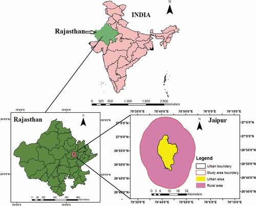
Jaipur (capital of the Rajasthan state in Northern India) is the 10^th largest city in India with geographical coordinates as 26° 25ʹ to 27° 51ʹ north latitude and 74° 55ʹ to 76° 10ʹ east longitude. In 2001, the urban population of Jaipur city was 2.3 million which has increased to 3.07 million in 2011 (Census of India 2011). Being heading to a metropolitan from developing city, Jaipur has been selected as the study area (Figure 1). The city is bound to have improved spatial growth in the coming decades to provide both economic as well as population growth (JDA 2011). In 2001, Jaipur Municipal Corporation (JMC) area spread over 462 sq. km. comprising of 70 wards, which have expanded by 5 sq. km. over the decade with 77 wards spreading across an area of 467 sq. km. in 2009. For studying various land uses pattern in this region, a study area of 12 km buffer outside urban area covering about approximately 1370 sq. km area has been considered. The main reason to consider this buffer is to incorporate both rural and urban area. The length and width of the urban area (hereafter referred as an urban boundary) are approximately 21 km in North-South direction and 13 km in East-West direction.

With varied topography; having Nahargarh hills in the north and Jhalana (a part of Aravalli hills) in the East, the growth of built-up area has been boosted mainly in the south, southwest and west.

Figure 1. Geographical location of Jaipur study area

2.2. Input data

2.2.1. For lands use/land cover classification

The multispectral cloud-free satellite imagery used for the present study has been procured from the website of United States Geological Survey (USGS). Land cloud coverage of the images is less than 10%. Table 1 and Table 2 show the remote sensing data used for the present work

Table 1. Remote sensing data used for the present work

Region	Satellite	Sensor	Acquisition date	Path and row	Spatial resolution (m)
Jaipur	Landsat	TM	October 2008	147 and 41	30
	Landsat	TM	October 2011	147 and 41	30

Survey of India (SOI) Topo sheets, bearing no: 45N/13, 45N/14, 45N/9 and 45N/10 with a scale 1:50,000 of Jaipur district and adjoining and Master plan of Jaipur (2011) was collected from the Jaipur development authority (JDA). Field data have been collected for identified sample sites for classification and as reference data for accuracy assessment of classified image. The fieldwork was conducted for sample sites identification during the year 2011.

2.2.2. For land surface temperature calculation

Available MODIS (Aqua) data for the year 2008 and 2011 for Jaipur have been downloaded from the website of LP DACC with the following specification (LP DAAC, 2015). Eight-day MYD11A2 LST product is available for both night and day time. It is calculated by averaging the view-time LST of two to eight days for clear-sky conditions (Wan 2007). It has 12 Science Data Sets (SDS) layers, which give day and night images of LST and information such as view angle, view time and clear sky conditions during the recording of LST observation, both for day time and night time LST. The 33 emissivities of bands 31 and 32, which have been used to derive LST, are also available as separate SDS layers.

The MODIS data are in HDF-EOS format and in Sinusoidal Projection System. Images were pre-processed using MODIS Re-Projection Tools (MRT) and are re-projected from Sinusoidal projection to UTM Zone 43N projection system with WGS84 as datum and reformatted from HDF-EOS to GeoTIFF format. A total of 40 images of night-time LST of summer (mid of March to June end) and winter season (November to February) with less than 10% cloud cover for two different stretches of time (2008 and 2011), respectively.

2.2.3. For ISA calculation

Landsat TM image of June 2008 and February 2011 have been selected for %ISA calculation. These images have been geometrically rectified to the Universal Traverse Mercator (UTM) projection system (datum WGS 84, Zone 43). The ground control points have been carefully selected to make sure that the RMS errors lies below 0.5 pixels.

2.3. Methodology

2.3.1. Data acquisition and scanning

Cloud free remote sensing data has been collected from various sources. Hard copy maps such as SOI topo sheet and Master plan of the three cities have been converted to digital maps by scanning in Joint Photographic Expert Group (JPEG) format.

2.3.2. Registration or geo-referencing

Data pre-processing including Registration (providing standard scale), Geo-referencing of image, rectification, and enhancement of data sets forms an integral component of processing workflow for the derivation of surface temperature map. Basic Remote Sensing Techniques followed are the Image pre-processing, processing and Interpretation and analysis using the software’s like ERDAS IMAGINE 9.2 Version and ArcGIS 10.0 Version.

2.3.3. Retrieval of the LST

LST obtained from 8 day MODIS night time MYD11A2 product is used for temperature pattern analysis of individual class in the study areas for 2 years (2008 & 2011). The average temperature of each LU-LC category for each season was calculated using the formula of simple arithmetic mean. The LST products used has a spatial resolution of 926.6 m as compared to Landsat TM 30 m spatial resolution. The LU-LC layers have been aggregated to match the resolution of LST images. The aggregation technique uses a specified statistical aggregation method within a neighborhood to derive values in the output raster at the different resolution. The aggregate tool of ArcGIS works by aggregating the individual values of a collection of cells and generating a single, coarser resolution cell of that value. The types of statistics available to aggregate the input values are Sum, Minimum, Maximum, Mean, and Median. In the present study mean aggregate is used.

2.3.4. LU-LC classification system

There are generally two kinds of classifications (1) Unsupervised Classification (2) Supervised Classification. The first type of classification involves just giving the number of classes to the software in which one wants to classify the land use classes. It is an experimental approach to classification. On the other hand, supervised classification requires some kind of supervision from users in the form of training samples. In this method, training samples are collected by the user for the training of classification algorithm. Supervised classification using Maximum Likelihood Classifier has been performed on a combination of bands on both images to map the land cover of the study area during both the years using ERDAS Imagine (Leica Geosystems Inc.).

2.3.4.1. Satellite imageries processing

Image rectification, data layer stacking to prepare false color composites (FCC) and resolution merge have been used to pre-process all the satellite imageries. Spectral profiles were generated to identify the differentiable LU-LC classes and separability of these classes in different spectral bands. Seven broad LU-LC types so identified are residential, commercial, industrial, roads, vegetation, soil (barren and loose soil), and water bodies.

2.3.4.2. Training of classification algorithm

Supervised classification requires training of classification algorithm for which training samples also known as signatures are needed to be collected for each targeted LU-LC class based on the prior knowledge of these classes. After selecting pixels for each class, separability matrix has been generated to find the optimum band combination in which all the LU-LC classes are separable for all the satellite imageries. Separability matrix evaluates the TD (Transformed Divergence) values for each class in different band combinations. Band combination with maximum TD value indicates the highest separability between the various LU-LC classes. Contingency matrix is generated and analyzed to check the misclassification among selected training pixels. It checks whether pixels selected for any particular class falls in other classes or not. If the percentage of error in the matrix is high, then signatures need to be refined. Histogram plotting is another way of examining the training samples for all the classes.

2.3.5. Evaluating impervious surfaces of the study area

Extraction of impervious surfaces at the subpixel level can be done by using the linear spectral mixture analysis (Wu and Murray 2003). The Linear spectral unmixing method has been used to extract impervious surfaces from the study area using ENVI 5.0 software. The analytical procedure for linear spectral mixture analysis is discussed below.

2.3.5.1. Water body masking

Modified Normalized difference water indices (MNDWI) have been used to extract water bodies from remote sensing data (Xu 2006) before conducting linear mixture spectral analysis (LMSA). The mathematical equation of MNDWI is given below.

(1) $\mathrm{M}\mathrm{N}\mathrm{D}\mathrm{W}\mathrm{I}=\frac{{\mathrm{R}}_{\mathrm{G}\mathrm{R}\mathrm{E}\mathrm{E}\mathrm{N}}-{\mathrm{R}}_{\mathrm{M}\mathrm{I}\mathrm{R}}}{{\mathrm{R}}_{\mathrm{G}\mathrm{R}\mathrm{E}\mathrm{E}\mathrm{N}}+{\mathrm{R}}_{\mathrm{M}\mathrm{I}\mathrm{R}}}$(1)

Where, ${\mathrm{R}}_{\mathrm{G}\mathrm{R}\mathrm{E}\mathrm{E}\mathrm{N}}$ = reflectance in green band

${\mathrm{R}}_{\mathrm{M}\mathrm{I}\mathrm{R}}$ = reflectance in mid infrared band

2.3.5.2. MNF transform

The maximum noise fraction (MNF) transformation places most of the variances of the spectral bands into the first two or three resultant components. It is an improved variant of Principle Component Analysis (PCA) by ordering components according to Signal-to-Noise Ratios (SNR) (Green et al. 1988).

2.3.5.3. Linear spectral unmixing

In order to perform linear unmixing model for the LMSA, four types of end members are selected in the present study: vegetation, low albedo, high albedo and soil by composing a scatter plot using the first two MNF components. Finally, constrained mixture spectral analysis has been used to process the pixel values of the masked image with the end member spectra. In the linear spectral unmixing model, the spectral value of an image pixel can be treated as a linear combination of different types of end members.

(2) ${\mathrm{R}}_{\mathrm{b}}=\sum _{\mathrm{i}=1}^{\mathrm{N}}{\mathrm{f}}_{\mathrm{i}}{\mathrm{R}}_{\mathrm{i},\mathrm{b}}+{\mathrm{e}}_{\mathrm{b}}$(2)

(3) $\mathrm{R}\mathrm{M}\mathrm{S}=\sqrt{\frac{{\sum }_{\mathrm{b}=1}^{\mathrm{M}}{\mathrm{e}}_{\mathrm{b}}^2}{\mathrm{M}}}$(3)

Where ${\mathrm{R}}_{\mathrm{b}}$= reflectance in band b

${\mathrm{f}}_{\mathrm{i}}$= fraction of end member in band b

${\mathrm{R}}_{\mathrm{i},\mathrm{b}}$= reflectance of end member in band b

${\mathrm{e}}_{\mathrm{b}}$= error in band

N = total number of endmembers

M = total number of bands

2.3.5.4. Endmember fractions

By resolving the LSMA model (Eq. (2(2) ${\mathrm{R}}_{\mathrm{b}}=\sum _{\mathrm{i}=1}^{\mathrm{N}}{\mathrm{f}}_{\mathrm{i}}{\mathrm{R}}_{\mathrm{i},\mathrm{b}}+{\mathrm{e}}_{\mathrm{b}}$(2) )) using the least error method, the pixel values of the masked TM sensor images can be separated into fractions for the four endmembers. As urban areas with a wide range of spectral properties, impervious surfaces possess both high and low albedo values. Therefore, a linear mixture of low albedo and high albedo can be considered as a good representation of imperviousness (Eq. (4(4) ${\mathrm{R}}_{\mathrm{i}\mathrm{m}\mathrm{p},\mathrm{b}}={\mathrm{f}}_{\mathrm{l}\mathrm{o}\mathrm{w}}{\mathrm{R}}_{\mathrm{l}\mathrm{o}\mathrm{w},\mathrm{b}}+{\mathrm{f}}_{\mathrm{H}\mathrm{i}\mathrm{g}\mathrm{h}}{\mathrm{R}}_{\mathrm{H}\mathrm{i}\mathrm{g}\mathrm{h},\mathrm{b}}+{\mathrm{e}}_{\mathrm{b}}$(4) )), and the fraction of impervious surface for each pixel can be estimated as the sum of fractions of high albedo and low albedo (Wu and Murray 2003).

(4) ${\mathrm{R}}_{\mathrm{i}\mathrm{m}\mathrm{p},\mathrm{b}}={\mathrm{f}}_{\mathrm{l}\mathrm{o}\mathrm{w}}{\mathrm{R}}_{\mathrm{l}\mathrm{o}\mathrm{w},\mathrm{b}}+{\mathrm{f}}_{\mathrm{H}\mathrm{i}\mathrm{g}\mathrm{h}}{\mathrm{R}}_{\mathrm{H}\mathrm{i}\mathrm{g}\mathrm{h},\mathrm{b}}+{\mathrm{e}}_{\mathrm{b}}$(4)

Where ${\mathrm{R}}_{\mathrm{i}\mathrm{m}\mathrm{p},\mathrm{b}}$,${\mathrm{R}}_{\mathrm{l}\mathrm{o}\mathrm{w},\mathrm{b}}$, ${\mathrm{R}}_{\mathrm{H}\mathrm{i}\mathrm{g}\mathrm{h},\mathrm{b}}$ = reflectance of impervious surfaces, low albedo and high albedo for band b; ${\mathrm{f}}_{\mathrm{l}\mathrm{o}\mathrm{w}}$,${\mathrm{f}}_{\mathrm{H}\mathrm{i}\mathrm{g}\mathrm{h}}$ = fraction of low albedo and high albedo; ${\mathrm{e}}_{\mathrm{b}}$ = error for band b.

2.3.5.5. Data analysis

LST and %ISA for individual LU-LC type are extracted using ArcGIS 10.0 software. This has been done by ‘Extract by Mask’ spatial analyst tool, in which the data layer to be extracted has been taken as the input raster, and study area boundary has been taken as the feature mask. The LST product has different resolution that LU-LC classes, so it is necessary to have all of them at the same resolution. Aggregation of LU-LC classes has been done by Aggregate-Generalization’ spatial analyst tool. The output value of each aggregated pixel is calculated as the mean of the value of input pixel.

3. Result and discussion

3.1. Image classification

Refined signatures were used for supervised classification using Maximum Likelihood Classification algorithm. Maximum Likelihood algorithm checks the highest probability of matching pixel values for each feature class among different pixels. Similar pixel values are assigned to the same feature class. Each class incorporates amalgamation of varied type of similar features like, Vegetation includes agricultural, forest and parks while soil includes barren land and open spaces. Residential area includes urban and rural settlement and roads category do include National highway, Main roads, rural paths, and railways. The classified images have been then assessed for accuracy based on a stratified random sampling of 210 reference pixels. Classification Accuracy assessments were done with the help of field knowledge, visual interpretation, referring Google Earth and high resolution (1m) data available for the cities on BHUVAN portal of NRSC. Table 3 presents the results of accuracy assessment of both the classified maps. High classification accuracy has been achieved for all the selected classes in both the classified maps. Kappa coefficient, which is a measure of the proportional (or percentage) improvement by the classifier over a purely random assignment to classes was found.

Table 2. Remote sensing data used for LST

Remote Sensing Product	Short Name	Sensor	Platform	Temporal Resolution	Spatial Resolution (m)
LST and Emissivity	MYD11A2	MODIS	Aqua	8 Day	926.6

Table 3. Classification accuracy assessment report for Jaipur study area

	2008		2011
Land Cover Class	Producer’s Accuracy	User’s Accuracy	Producer’s Accuracy	User’s Accuracy
Residential	84.91%	92.00%	100.00%	80.00%
Industrial	100.00%	70.00%	83.33%	75.00%
Commercial	87.50%	77.33%	72.53%	80.55%
Roads	87.50%	70.00%	83.33%	90.00%
Soil	80.67%	95.00%	78.92%	98.00%
Vegetation	83.33%	100.00%	80.00%	100.00%
Water	90.91%	100.00%	100.00%	100.00%
Over All Accuracy	84.29%		86.58%
Kappa Statistic	0.8167		0.8342

Since the kappa value of the images lies between 0.80–0.85; the classification results have been accepted for further analysis. Fleiss’s (1981) equally arbitrary guidelines characterize Kappa’s over 0.75 is considered as excellent, values between 0.40 and 0.75 as fair to good, and below 0.40 as poor.

3.2. Spatial patterns of LU-LC

Figure 2 (a,b) show the spatial distribution of LU-LC in the study area in the year 2008 and 2011 respectively. Classified images have been compared visually as well as quantitatively to detect and measure the patterns and magnitude of changes in LU-LC categories occurred from 2008 and 2011.

Figure 2. Land use land cover maps of Jaipur study area (a) 2008 (b) 2011

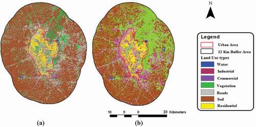
Results indicate that built-up areas have shown evident increment over a short period in the form of physical expansion as well as internal densification. The transition has been seen from vacant land to low dense built-up area. Such a rapid conversion of pervious areas into impervious areas leads to the different type of adverse hydrological impacts leading to problems of floods, drought and groundwater depletion. Imbalance in urban density for the study area is contributing towards problems like water shortage and depletion of local water sources, i.e., lakes due to change in watershed characteristics, pollution and increase in the risk of a heatwave. Enhanced surface temperature and urban heat island are another possible outcomes of unsustainable and unplanned urban growth. Table 4 shows the area (km²) of various land covers for the years 2008 and 2011. Built-up area has increased by about 21% between 2008 and 2011. Vegetation area has increased by about 12% between 2008 and 2011 whereas the soil area has decreased by about 6% between 2008 and 2011.

Table 4. Area (km²) of various land covers for different time periods

Category	2008	2008 (Number of pixels)	2011	2011 (Number of pixels)	% of increase in land covers
Built-up	150.24	175	181.64	212	0.21
water	1.53	2	4.66	5	2.05
soil	985.95	1148	923.35	1075	−0.06
vegetation	232.67	271	260.74	304	0.12
Total	1370.39	1596	1370.39	1596	-

3.3. LST pattern and UHI intensity of Jaipur study area

Figure 3 shows the 8-day night LST images of summer and winter season in the study area for two different stretches of time (2008 and 2011), respectively.

Figure 3. MODIS LST images of Jaipur study area for the years 2008 and 2011

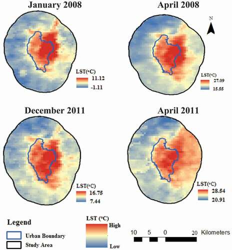
Higher temperature appears in the pixel within the urban boundary than the rural area, thereby showing the presence of SUHI. Eastern part of urban boundary exhibits higher temperature due to the presence of concentrated built-up area and Aravalli hill region as mining activities associated with this area have caused direct exposure of rocky area to sunlight. The urban area near the Eastern side of urban boundary encounters maximum LST. This part of the urban area has predominantly built-up and paved areas, and consequently, the nighttime LST of this area is the highest in the night images during all the seasons. Some part of the rural area, near this part and outside the urban boundary, corresponds to Aravalli hill range and this part also has some high-temperature pixels. Mining has been done in this region to meet the demand for stones for construction purposes that has resulted in rock surfaces being exposed to direct solar radiation. The energy interaction of rocks is similar to that of built-up area thereby resulting in high temperature in this region. Out of the two seasonal imagery better appearance of SUHI is seen in winter images in the form of contrasting color representing low and high temperature. Mean LST ranged from 2.69 to 24.27 °C across the study area in the year 2008. The maximum LST varies from 27.09 to 21.21 °C in summer and 16.05 to 8.91 °C in winter for the year 2008. While, the minimum LST values ranges from 8.57 to 21.75 ^oC in summer and from −1.19 to 6.03 ^oC in winter for 2008. Mean LST in the region recorded a significant increase (p < 0.05) of approximately 2 °C in 2011. It ranged from 4.33 to 25.94 °C across the city. P- Test has been conducted to get the p value less than 0.05 where p value obtained is 0.0256 and the total number of observation (N) is 100. The maximum LST during summer and winter varies from 29.93 to 18.09 °C and from 16.75 to 8.65 °C, respectively, and the minimum LST ranges from 8.69 to 22.69 °C in summer and 2.09 to 7.57 °C in winter. The magnitude of SUHI can be expressed in terms of intensity, which is the difference between urban and rural LST (Clinton and Gong 2013). SUHI intensity is calculated as the difference in temperature between two points, within the area of interest, during simultaneous observations. SUHI intensity when recorded on the basis of maximum and minimum temperatures, it is called maximum SUHI intensity. The existing surface temperature pattern has been intensifies over the period of time. The overall maximum UHI intensity out of the two seasons is recorded as 12.64 °C during the summer season of 2008. The UHI intensity was found to range from 5.12 to 12.64 °C during 2008 which foresees an increase in the temperature range from 2008 to 2011 owing to enhanced LST. UHI intensity ranged from 6.50 to 13.68 °C during 2011. In general, SUHI is not apparent at daytime. SUHI varies during the day, and it is more significant during the evening/night (Mathew et al. 2017). Hence, night time LST analysis has been carried out for SUHI assessment.

3.4. Temperature variations for different land cover types

The best way to understand the influence and contribution of LU-LC on LST is to investigate the connection between the thermal signatures (i.e., the LST profile of the study area) and individual land cover type, Weng (2001). Temperature of each LU-LC form had been calculated individually for summer and winter season and then the daily and seasonal average were calculated to find the temperature variations. Table 5 gives the mean seasonal LST for different landforms during the two years. Results revealed that high LST are associated with built-up area; Residential area shows the highest temperature while bare soil and open land record lowest LST. Packed and concentrated old city area reflects high temperature while the upcoming infrastructural residential projects aiming to accommodate the increasing population of Jaipur city shows highest increase in temperature. LST is very sensitive to various land features and hence can be used to extract information on different LU-LC features (Sinha et al. 2015).

Figure 4. Variation of the mean LSTs and the UHI intensities by classes and seasons (2008)

Figure 5. Variation of the mean LSTs and the UHI intensities by classes and seasons (2011)

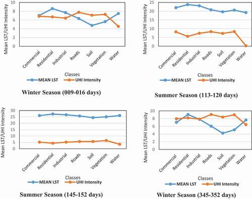
Table 5. Average LST (^oC) corresponding to different land use types over Jaipur study area

	2008		2011
CLASS	Summer	Winter	Summer	Winter
Commercial	20.53	7.45	21.64	9.88
Residential	21.76	9.29	23.21	11.46
Industrial	21.39	8.73	22.38	10.59
Roads	19.44	6.16	21.01	9.03
Soil	18.48	4.91	19.42	7.52
Vegetation	19.31	6.17	20.24	8.30
Water	18.35	5.23	21.38	10.10

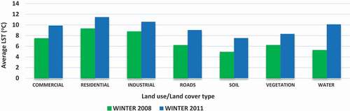
Figures 4 and 5 represent the fluctuation of the mean LSTs and the UHI intensities (^oC) over Jaipur study area corresponding to different land use types for different seasons of the years 2008 and 2011, respectively. Table 6 shows the number of pixels of various land cover categories. The average surface temperature of the different LU-LC category of the study area has shown an appreciable increment for both the seasons from 2008 to 2011. Table 5 shows the average LST (^oC) corresponding to different land use types over Jaipur study area. For summers, the average LST has shown a rise of 1.45 °C in residential area, 1.11 °C in commercial, 0.99 °C in industrial, 1.87 °C in roads, 0.94 °C in soil, 0.93 °C in vegetation and 3.03 °C in water from 2008 to 2011. The findings for winter season also shows enhanced mean LST for every area LU-LC category like a rise of about 2.17 °C has been seen in residential areas, 2.46 °C in commercial, 1.86 °C temperature rise in industrial, 2.87 °C in roads; a rise of 2.55, 2.13, 3.82 °C has also been seen in soil, vegetation and water LU-LC type, respectively. The rise in average LST for all feature classes was found to be more in winter season as compared to the summer season from 2008 to 2011, consequently demonstrating the warming of the area over the time because of imperviousness, anthropogenic exercises, lessening in vegetation and so forth. The reflection of appreciable temperature rise in built-up area could be because of the densification of the already existing built-up area and new land transformation which could be seen in the central and northern part of the city. Densification of study area is increase in ISA and it is directly proportional to the population growth. Densification mainly focusses on urban sprawl and increase in built-up density over the study area. Extreme north- eastern part shows a change of densely vegetated area into the vacant land which also corresponds to the transition of the area from lower to higher LST category. Figures 6 and 7 show the variations and help in understanding the contribution of each land use type on LST seasonally.

Figure 6. Variations of mean LST for different LULC type from 2008 to 2011 during summer

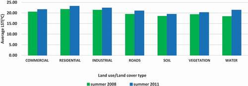
Table 6. Number of pixels of various land cover categories

CLASS	2008 (Number of pixels)	2011 (Number of pixels)
Residential	81	96
Industrial	27	36
Roads	19	24
Soil	1148	1075
Vegetation	271	304
Water	2	5

In this study, it has been observed that LST is showing higher values even with an increment in vegetation coverage. It is also observed that vegetation increment mainly observed in the Eastern part of the study area (Aravalli hill ranges). Aravalli hill ranges comprise of exposed rocks. Even the Aravalli hill ranges covered with vegetation cover, the exposed rocks which have caused direct exposure of rocky area to sunlight. This will result in higher LST over the area due to the presence of exposed rocks which increase the ISA over the area also. During night, water bodies’ thermal characteristics are similar to built-up areas. Water bodies show higher LST especially during night because whatever the thermal energy absorbed during day period will emit during the night period to maintain the thermal equilibrium. In this aspect, water features showed increased LSTs, also as the water area increased, LST range also increased.

Figure 7. Variations of mean LST for different LU-LC type from 2008 to 2011 during winter

3.5. Percentage imperviousness surface area and its variation for different land cover types

% ISA images for different period showing ISA values ranging between 0 and 100% are shown in Figure 8.

Figure 8. Landsat % ISA images of the study area

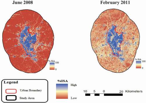
The overall absolute maximum and minimum value obtained are 100 and 0% while the range between 0 and 100 shows imperviousness increasing from 0 to 100. The area with blue color represents the high imperviousness within the urban boundary, which seems to have enhanced over the period of time. The imperviousness in the form of % ISA has been obtained for both the years, since the scale value for both the LU-LC map and imperviousness map are same; the extraction of information could be easily carried out. Table 7 shows the % ISA values for individual land use type during 2008 and 2011. Since % ISA is independent of seasonal variation; hence, random selection of image was done for %ISA calculation.

Figure 9. Variations of % ISA over different land cover types

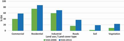
Table 7. % ISA variation over Jaipur study area for different land cover type

Class	%ISA (2008)	%ISA (2011)
Commercial	39.43	57.97
Residential	74.06	86.49
Industrial	59.01	69.25
Roads	15.84	36.45
Soil	1.92	18.40
Vegetation	8.75	22.66

Figure 9 helps in better visualization of the disparity between the impervious surfaces for two study period. Even though we have LU-LC map with seven different classes, but water bodies are exempted from imperviousness analysis. Considered as purely non-urban areas, it was reclassified to 0% impervious class. On close analysis of the trend for %ISA shown in the bar graph, it is observed that imperviousness has increased over the course of time. The increase in impervious surfaces dominates in roads, soil, commercial, residential, industrial, and vegetation in descending order. An increase of 20.61, 16.48, 18.54, 12.43, 10.24, and 13.91% in roads, soil, commercial, residential, industrial, and vegetation-land use types is seen, respectively. The numbers themselves show densification of the existing built-up area with new commercial and residential area or mixed from of both coming up in recent time. Moreover, construction and widening of roads in the region also contributed to the imperviousness. The decrement in protective vegetation cover in the central region as well in the rural area can also be seen which seem to be an important reason for enhanced temperature due to land form transformation. Yuan and Bauer (2007) have reported a strong relationship between the amount of ISA and surface temperatures or the UHI effect, which is also validated by the present study. Hence, it helps us in understanding that increased impervious surfaces have played a major role in rising average surface temperature of Jaipur and adjoining area.

4. Conclusion

Major studies regarding UHI relationship with LU-LC tell us the growth pattern of the individual LU-LC type but not about their individual contribution on enhanced surface temperature or resulting phenomenon of UHI. The present study documents this gap and shows some specific contributing temperature values. It also helps in understanding that there is an urgent need to focus on the growth and establishment pattern of the area. Eight-day night time MODIS LST has been used for the analysis of the LU-LC effect on LST of Jaipur city. The LU-LC classification maps generated for the study area classify the study area into seven different classes as residential, commercial, industrial, roads, soil, vegetation, and water. The study reveals that the residential area shows the highest mean LST for both the seasons during 2008 and 2011 owing to new construction and densification of existing areas. On the other hand, soil shows the minimum temperature in the study area owing to a unique property of soil to get heated up quickly and quickly cool down, thereby retaining less heat than the anthropogenic materials. The areas within urban boundary show higher temperature than the rural area; thus, supporting the existence of SUHI effect. Another interesting conclusion drawn from the comparison of temperature of various land use types seasonally is that winter temperature of each land use type shows a greater hike than summer temperatures from 2008 to 2011. The average rise for seven categories in temperature during winter season was found to be around 2.6 while 1.47 °C rise was observed during summers. The study also observes an increase in % ISA in all the classes over the duration of the study period. Enhanced imperviousness supports the temperature variations in different classes from 2008 to 2011.

Acknowledgements

This work was supported by the Department of Science and Technology (DST) Delhi, Government of India. The authors would like to thank the anonymous reviewers for their instructive comments, which helped to improve this article. The authors wish to thank the Land Processes Distributed Active Archive Center (LP DAAC), located at the U.S. Geological Survey (USGS) Earth Resources Observation and Science (EROS) Center (lpdaac.usgs.gov) for making available the satellite data.

Disclosure statement

No potential conflict of interest was reported by the authors.

Additional information

Funding

This work was supported by the Science and Engineering Research Board.

Notes on contributors

Neha Gupta

Neha Gupta received the M. Tech. degree (with gold medal) in water resources engineering from Malaviya National Institute of Technology Jaipur, Jaipur, India, in 2015. Currently, she is pursuing the Ph.D. degree in civil engineering at the Indian Institute of Technology Ropar. Her research interests include water resources engineering, groundwater hydrology, urban sprawl, land use/ land cover modeling, remote sensing and GIS applications in water resources and climate change, modeling for urban planning applications, urban heat island, and climate change.

Aneesh Mathew

Aneesh Mathewreceived the B. Tech. degree in civil engineering from Mahatma Gandhi University, Kerala, India, in 2011, and the M. Tech. degree (with gold medal) in water resources engineering from Malaviya National Institute of Technology Jaipur, Jaipur, India, in 2014. He has completed the Ph.D. degree in civil engineering from Malaviya National Institute of Technology Jaipur in 2018. Currently, he is working as a Sr. Assistant Professor with the Department of Civil Engineering, Madanapalle Institute of Technology & Science, Madanapalle. His research interests include water resources engineering, image processing, digital elevation models, remote sensing and GIS applications in water resources and climate change, modeling for urban planning applications, urban heat island, and climate change.

Sumit Khandelwal

Sumit Khandelwal received the B. Tech. Degree (with gold medal) from Jai Narayan Vyas University, Jodhpur, India, in 1997, and the M.Tech. degree in water resources engineering and the Ph.D. degree in civil engineering from Malaviya National Institute of Technology Jaipur, Jaipur, India, in 2002 and 2012, respectively. Currently, he is an Associate Professor with the Department of Civil Engineering, Malaviya National Institute of Technology Jaipur. His research interests include remote sensing and GIS applications in water resources and climate change especially urban heat island, climate change and urban sprawl, air pollution monitoring, and modeling.

References

- Ahmed B, Kamruzzaman M, Xuan Z, Rahman S, Choi K. 2013. Simulating land cover changes and their impacts on land surface temperature in Dhaka, Bangladesh. Remote Sens Environ. 5:5969–5998. ISSN 2072-4292. doi:https://doi.org/10.3390/rs5115969.
- Akbari H, Konopacki S. 2005. Calculating energy-saving potentials of heat-island reduction strategies. Energy Policy. 33:721–756.
- Alshaikh AY. 2015. Space applications for drought assessment in wadi-dama (West Tabouk), KSA. Egypt J Remote Sens Space Sci. 18:543–553.
- Amanollahi J, Tzanis C, Ramli MF, Abdullah AM. 2016. Urban heat evolution in a tropical area utilizing Landsat imagery. Atmos Res. 167:175–182.
- Babalola OS, Akinsanola AA. 2016. Change detection in land surface temperature and land use land cover over lagos metropolis, Nigeria. J Remote Sens GIS. 5:1–7.
- Bokaie M, Zarkesh MK, Arasteh PD, Hosseini A. 2016. Assessment of urban heat island based on the relationship between land surface temperature and land use/land cover in Tehran. Sustainable Cities Soc. 23:94–104.
- Bonafoni S, Anniballe R, Pichierri M. 2015. Comparison between surface and canopy layer urban heat island using MODIS data. Joint Urban Remote Sens Event (JURSE). Lausanne. 1–4. doi:https://doi.org/10.1109/JURSE.2015.7120457.
- Borbora J, Das AK. 2014. Summertime urban heat island study for Guwahati city, India. Sustainable Cities Soc. 11:61–66.
- Census of India. 2011. District census handbook, Town directory of Jaipur, Directorate of Census Operations, Rajasthan, India.
- Chen XL, Zhao HM, Li PX, Yin ZY. 2006. Remote sensing image-based analysis of the relationship between urban heat island and land use/cover changes. Remote Sens Environ. 104(2):133–146.
- Clinton N, Gong P. 2013. MODIS detected surface urban heat islands and sinks: global locations and controls. Remote Sens Environ. 134:294–304.
- Deng Y, Wang S, Bai X, Tian Y, Wu L, Xiao J, Chen F, Qian Q. 2018. Relationship among land surface temperature and LUCC, NDVI in typical karst area. Sci Rep. 8:1–12.
- Dousset B, Gourmelon F. 2003. Satellite multi-sensor data analysis of urban surface temperatures and land cover. ISPRS – J Photogramm Remote Sens. 58(1–2):43–54.
- Efstathiou MN, Tzanis C, Cracknell AP, Varotsos CA. 2011. New features of land and sea surface temperature anomalies. Int J Remote Sens. 32:3231–3238.
- Fleiss JL. 1981. Statistical methods for rates and proportions. 2nd ed. New York: John Wiley; pp. 38–46.
- Green AA, Berman M, Switzer P, Craig MD. 1988. A transformation for ordering multispectral data in terms of images quality with implications for noise removal. IEEE Trans Geosci Remote Sens. 26(1):65–74.
- Guo G, Wu Z, Xiao R, Chen Y, Liu X, Zhang X. 2015. Impacts of urban biophysical composition on land surface temperature in urban heat island clusters. Landsc Urban Plan. 135:1–10.
- Hung T, Uchihama D, Ochi S, Yasuoka Y. 2006. Assessment with satellite data of the urban heat island effects in Asian mega cities. Int J Appl Earth Obs Geoinf. 8(1):34–48.
- Imhoff ML, Zhang P, Wolfe RE, Bounoua L. 2010. Remote sensing of the urban heat island effect across biomes in the continental USA. Remote Sens Environ. 114:504–513.
- Jalan S, Sharma K (2014). Spatio-temporal assessment of land use/land cover dynamics and urban heat island of Jaipur city using satellite data. The International Archives of the Photogrammetry, Remote Sensing and Spatial Information Sciences, Volume XL-8, ISPRS Technical Commission VIII Symposium, Dec 09–12, Hyderabad, India
- JDA. 2011. Master plan handbook. Jaipur (Rajasthan, India): Jaipur Development Authority.
- Jin M, Dickinson RE, Zhang D-L. 2005. the footprint of urban areas on global climate as characterized by MODIS. J Clim. 18:1551–1565.
- Klok L, Zwart S, Verhagen H, Mauri E. 2012. The surface heat island of rotterdam and its relationship with urban surface characteristics. Resources, Conservation and Recycling. 64:23–29.
- Landsberg HE. 1981. The urban climate. In: International geographic series. Vol. 28. New York: Academic Press; p. 275.
- Li. T, Chen J, Yu S. 2013. How has Shenzhen been heated up during the rapid urban build-up process? Landsc Urban Plan. 115:18–29.
- Li Y, Zhang H, Kainz W. 2012. Monitoring patterns of urban heat islands of the fast-growing Shanghai metropolis, China: using time-series of landsat TM/ETM+ data. Int J Appl Earth Obs Geoinf. 19:127–138.
- Liang BQ, Weng QH. 2011. Assessing urban environmental quality change of Indianapolis (1998) United States, by the remote sensing and GIS integration. IEEEJ Sel Top Appl Earth Observ Remote Sens. 4(1):43–55.
- LPDAAC. 2015. MODIS overview, USGS website. URI: https://lpdaac.usgs.gov/dataset_discovery/modis/modis_products_table
- Mackey CW, Lee X, Smith RB. 2012. Remotely sensing the cooling effects of city scale efforts to reduce urban heat island. Build Environ. 49:348–358.
- Mathew A, Khandelwal S, Kaul N. 2016. Spatial and temporal variations of urban heat island effect and the effect of percentage impervious surface area and elevation on land surface temperature: study of Chandigarh city, India. Sustainable Cities Soc. 26:264–277.
- Mathew A, Khandelwal S, Kaul N. 2017. Analysis of diurnal surface temperature variations for the assessment of surface urban heat island effect over Indian cities. Energy Build. 159:271–295.
- Mathew A, Khandelwal S, Kaul N. 2018. Investigating spatio-temporal surface urban heat island growth over Jaipur city using geospatial techniques. Sustainable Cities Soc. 40:484–500.
- McMichael AJ, Woodruff RE, Hales S. 2006. Climate change and human health: present and future risks. Lancet. 367:859–869.
- Mohan M, Pathan SK, Narendrareddy K, Kandya A, Pandey S. 2011. Dynamics of urbanization and its impact on land-use/land-cover: a case study of megacity Delhi. J Environ Prot. 2:1274–1283.
- Montavez JP, Rodriguez A, Jimenez JI. 2000. A study of the urban heat island of Granada. Int J Climatol. 20:899–911.
- Pal S, Ziaul S. 2016. Detection of land use and land cover change and land surface temperature in english bazar urban centre. Egypt J Remote Sens Space Sci. 20:125–145.
- Patki NP, Alange PR. 2008. Study of influence of land cover on urban heat islands in pune using remote sensing. IOSR J Mech Civ Eng (IOSR-JMCE). 39–43 ISSN: 2278-1684.
- Peng S, Piao S, Ciais P, Friedlingstein P, Ottle C, Breon FM, Nan HJ, Zhou LM, Myneni RB. 2012. Surface urban heat island across 419 global big cities. Environ Sci Technol. 46:696–703.
- Qiao Z, Tian G, Xiao L. 2013. Diurnal and seasonal impacts of urbanization on the urban thermal environment: a case study of Beijing using MODIS data. ISPRS J Photogramm Remote Sens. 85:93–101.
- Quattrochi DA, Luvall JC. 1999. Thermal infrared remote sensing for analysis of landscape ecological processes: methods and applications. Landsc Ecol. 14:577–598.
- Rajasekar U, Weng Q. 2009. Urban heat island monitoring and analysis using a non-parametric model: a case study of Indianapolis. ISPRS J Photogramm Remote Sens. 64:86–96.
- Rotem-Mindali O, Michael Y, Helman D, Lensky IM. 2015. The role of local land-use on the urban heat island effect of Tel Aviv as assessed from satellite remote sensing. Appl Geogr. 56:145–153.
- Seto KC, Shepherd JM. 2009. Global urban land-use trends and climate impacts. Curr Opin Environ Sustain. 1:89–95.
- Singh RB, Grover A, Zhan J. 2014. Inter-seasonal variations of surface temperature in the urbanized environment of Delhi using landsat thermal data. Energies. 7:1811–1828.
- Sinha S, Sharma LK, Nathawat MS. 2015. Improved land-use/land-cover classification of semi-arid deciduous forest landscape using thermal remote sensing. Egypt J Remote Sens Space Sci. 18:217–233.
- Stewart ID, Oke TR. 2012. Local climate zones for urban temperature studies. Bull Am Meteorol Soc. 93(12):1879–1900.
- Streutker DR. 2002. A remote sensing study of the urban heat island of Houston, Texas. Int J Remote Sens. 23(13):2595–2608.
- Tran H, Uchihama D, Ochi S, Yasuoka Y. 2006. Assessment with satellite data of the urban heat island effects in Asian mega cities. Int J Appl Earth Obs Geoinf. 8(1):34–48.
- United Nations. 2010. Department of economic and social affairs, population division. World urbanization prospects: The 2009 revision; 2010. CD-ROM edition data in digital form − (POP/DB/WUP/Rev.2009).
- Van De Kerchove R, Lhermitte S, Veraverbeke S, Goossens R. 2013. Spatio-temporal variability in remotely sensed land surface temperature, and its relationship with physiographic variables in the Russian Altay Mountains. Int J Appl Earth Obs Geoinf. 20:4–19.
- Voogt JA, Oke TR. 2003. Thermal remote sensing of urban climates. Remote Sens Environ. 86:370–384.
- Wan Z. 2007. Collection-5, MODIS land surface temperature products users’ guide, (ICESS, university of California, Santa Barbara). http://www.icess.ucsb.edu/modis/LstUsrGuide/MODIS_LST_products_Users_guide_C5.pdf
- Weng Q. 2001. A remote sensing-GIS evaluation of urban expansion and its impact on surface temperature in Zhujiang Delta, China. Int J Remote Sens. 22(10):1999–2014.
- Weng Q, Liu H, Lu D. 2007. Assessing the effects of land use and land cover patterns on thermal conditions using landscape metrics in city of Indianapolis, United States. Urban Ecosyst. 10:203–219.
- Weng QH, Fu P. 2014. Modeling diurnal land temperature cycles over Los Angeles using downscaled GOES imagery. ISPRS J Photogramm Remote Sens. 97(97):78–88.
- Weng QH, Liu H, Liang BQ, Lu DS. 2008. The spatial variations of urban land surface temperatures: pertinent factors zoning effect, and seasonal variability. IEEE J Sel Top Appl Earth Observ Remote Sens 1(2):154–166.
- Weng QH, Lu DS. 2008. A sub-pixel analysis of urbanization effect on land surface temperature and its interplay with impervious surface and vegetation coverage in Indianapolis United States. Int J Appl Earth Obs Geoinf. 10(1):68–83.
- World Health Organization. 2010. Centre for health development, united nations human settlements programme. Hidden cities: Unmasking and overcoming health in equities in urban settings: Un-habitat.
- Wu C, Murray AT. 2003. Estimating impervious surface distribution by spectral mixture analysis. Remote Sens Environ. 84:493–505.
- Wu H, Lu-Ping Y, Wen-Zhong Shi, Clarke KC. 2014. Assessing the effects of land use spatial structure on urban heat islands using HJ-1B remote sensing imagery in Wuhan, China. Int J Appl Earth Obs Geoinf. 32:67–78.
- Xiao H, Weng Q. 2007. The impact of land use and land cover changes on land surface temperature in a karst area of China. J Environ Manage. 85:245–257.
- Xu HQ. 2006. Modification of Normalized Difference Water Index (NDWI) to enhance open water features in remotely sensed imagery. Int J Remote Sens. 27(14):3025–3033.
- Yuan F, Bauer ME. 2007. Comparison of impervious surface area and normalized difference vegetation index as indicators of surface urban heat island effects in Landsat imagery. Remote Sens Environ. 106:375–386.
- Yue W, Xu J, Tan W, Xu L. 2007. The relationship between land surface temperature and NDVI with remote sensing: application to Shanghai Landsat 7 ETM+ data. Int J Remote Sens. 28:3205–3226.
- Zhang H, Qi Z, Ye XY, Cai YB, Ma W-C, Chen NM. 2013. Analysis of land use/land cover change, population shift, and their effects on spatiotemporal patterns of urban heat islands in metropolitan Shanghai, China. Appl Geogr. 44:121–133.
- Zhang Y, Inakwu O, Odeh A, Han C. 2009. .Bi-temporal characterization of land surface temperature in relation to impervious surface area, NDVI and NDBI, using a sub-pixel image analysis. Int J Appl Earth Obs Geoinf. 11:256–264.
- Zubair AO. 2006. Change detection in land use and land cover using Remote Sensing data and GIS (A case study of Ilorin and its environs in Kwara State.), Department of Geography, University of Ibadan.