Methods for Non-Compartmental Pharmacokinetic Analysis With Observations Below the Limit of Quantification

Abstract

Pharmacokinetic (PK) studies are conducted to learn about the absorption, distribution, metabolism, and excretion processes of an externally administered compound by measuring its concentration in bodily tissue at a number of time points after administration. Two methods are available for this analysis: modeling and non-compartmental. When concentrations of the compound are low, they may be reported as below the limit of quantification (BLOQ). This article compares eight methods for dealing with BLOQ responses in the non-compartmental analysis framework for estimating the area under the concentrations versus time curve. These include simple methods that are currently used, maximum likelihood methods, and an algorithm that uses kernel density estimation to impute values for BLOQ responses. Performance is evaluated using simulations for a range of scenarios. We find that the kernel based method performs best for most situations. Supplementary materials for this article are available online.

keywords:

• Below limit of quantification
• Kernel density estimation
• Noncompartmental analysis
• Pharmacokinetics

1 Introduction

In pharmacokinetic (PK) studies, the objective is to learn about the absorption, distribution, metabolism, and excretion (ADME) processes of an externally administered compound by measuring the concentration in bodily tissue such as blood or plasma at a number of time points after administration. However, some of these concentrations are reported as below the limit of quantification (BLOQ) of the assay. The limit of quantification (LOQ) is defined by Armbruster and Pry (2008) as “The lowest concentration at which the analyte can not only be reliably detected, but at which some predefined goals for bias and imprecision are met.” Observations that are below the LOQ are often referred to as “BLOQ” or “BQL” and require special attention in the data analysis.

Dealing with BLOQ observations when modeling is used has been vastly explored in the literature. The most notable of which is the contribution from Beal (2001), describing seven key methods for fitting PK models when BLOQ observations are present. Wang (2015) discusses the implications of such methods from the FDA perspective, an important contribution since the handling of such values must be regulated in practice. Further, regulatory requirements (Gabrielsson and Weiner 2001; Reisfield and Mayeno 2013; Dykstra et al. 2015) require many PK studies to use non-compartmental analysis (NCA), yet statistical methods for dealing with BLOQ observations in NCA are very much lacking.

The two strategies of PK analysis, modeling (e.g., Davidian and Giltinan 1995; Bonate 2006) and NCA (Gibaldi and Perrier 1982; Cawello 2003; Jaki and Wolfsegger 2012) differ in their approach on a number of levels. While the modeling approach offers the advantage of unstructured sampling schemes (i.e., fewer restrictions on the sparsity and structure of the sampling schedule), this comes at the cost of uncertainty over the model choice and potential technical difficulties in fitting the PK model. Many of the methods discussed by Beal (2001) involve either discarding BLOQ observations, replacing them with LOQ/2 or replacing them with 0 before proceeding to fit a PK model using such methods as maximum likelihood or least squares regression. Assumptions must be made about the underlying ADME process to use these approaches, as PK modeling involves representing the body as various compartments and modeling the flow of the compound between these compartments using differential equations. The number of compartments and hence complexity of the model used depends on the compound itself. Further, assumptions on the rate of flow between compartments must also be made and therefore the model choice is heavily dependent on assumptions on the compound being studied. In NCA, however, no such assumptions must be made, although some kind of approximation, usually linear or exponential decay, of the concentrations between observed time points is used. The purpose of both approaches is to estimate PK parameters such as the area under the concentration versus time curve (AUC), a measure of total exposure of the compound, or the maximum concentration of the compound ($C_{\max }$).

Figure 1 shows an illustration of a motivating example from a PK study of seven rats given an oral dose of a compound. The large gray numbers indicate that a response is reported as BLOQ, when the LOQ is defined at 5. This gives 5 BLOQ values in the dataset, out of 42 total observations. Here, a linear approximation between the observations at consecutive timepoints.

Fig. 1 An example dataset.

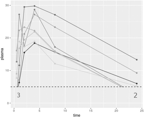
When there are a large number of responses BLOQ, and those responses that are above have low concentration values, the contribution of the BLOQ responses will vastly affect any estimate of the AUC and its variance; this is the PK parameter that is most affected by how BLOQ responses are dealt with. Johnson (2018) consider methods building on those introduced by Beal (2001) for example with small numbers of BLOQ values, including the potential to use the actual reported concentration values that are BLOQ. The residual error model that must be assumed for this method is not appropriate however for examples with larger numbers of BLOQ values. Conventional methods for dealing with missing data such as those introduced by Rubin (1987) and further explored by Little and Rubin (2002) are not applicable in this setting since the mechanism for the missingness does not follow the standard settings. In the following, we introduce eight methods for including BLOQ observations in NCA for PK studies, and hence make as few assumptions on the data as possible.

2 Methods

We introduce eight methods for dealing with values BLOQ and subsequently focus on how each of the methods impacts the estimate of the AUC, $\widehat{\text{AUC}}$, and its variance. We focus on complete sampling designs in our evaluations, although the methods may be extended to sparse sampling schemes, see Section 4, without further complication. The first two methods are simple imputations, replacing the BLOQ observations with 0 and LOQ/2 and proceeding with the NCA approach. These are the current approaches applied in practice (Hing et al. 2001) and hence the benchmark upon which we wish to improve on. The remaining six methods use varying techniques to either impute values onto BLOQ responses or to approximate the summary statistics of the non-compartmental approximation of the concentration versus time curve. It is worth noting that although in the following descriptions, we use a linear approximation between observations of consecutive timepoints, that is, the trapezoidal rule, one may also use the log-linear trapezoidal rule. In fact, any appropriate approximation between observations may be used as none of the following methods make any assumptions on this relationship. However, when approximating the variance of the $\widehat{\text{AUC}}$ obtained through such methods, this is easily approximated from estimates using the trapezoidal and log-trapezoidal rule, as described by Gagnon and Peterson (1998) and may not be so easily estimated for alternative approximations.

For all methods, two different error structures, additive and multiplicative are considered. We assume concentrations from n subjects, labeled $i=1,\dots ,n$, are observed at J timepoints t_j for $j=1,\dots ,J$.

2.1 Additive Error Model

The additive error model is defined as $$y_{ij}={\mu }_j+{ϵ}_{ij},$$ where y_ij is the observed response for subject i at the jth timepoint. The μ_j represents the population mean response at the jth timepoint. ϵ_ij is the difference between the y_ij and μ_j and is assumed to be normally distributed. In this case, we use the arithmetic mean $\overline{y_j}=\frac{1}{n}{\sum }_{i=1}^n{y}_{ij}$ as the basis for estimating the AUC. Assuming all observations were above the LOQ, the estimate of the population AUC is written as (1) $${\widehat{\text{AUC}}}^{(A)}=\sum _{j=1}^J{\omega }_j\overline{y_j},$$(1) where $\overline{y_j}$ is defined as above and ω_j are weights defined as $$\begin{array}{c}{\omega }_j=\frac{t_{j+1}-t_{j-1}}{2}\hspace{1em}\text{for}\hspace{1em}j=1,2,\dots ,(J-1),\\ =\frac{t_J-t_{j-1}}{2}\hspace{1em}\text{for}\hspace{1em}j=J.\end{array}$$

The variance approximation of the $\widehat{\text{AUC}}$ for batch designs (Jaki and Wolfsegger 2012) can be used: (2) $$\text{var}\left({\widehat{\text{AUC}}}^{(A)}\right)=\sum _{b=1}^B\frac{s_b^2}{n_b},$$(2) where $$s_b^2=\frac{1}{n_b-1}\sum _{i=1}^{n_b}{\left(\sum _{j\in J_b}{\omega }_j{y}_{ij}-\frac{1}{n_b}\sum _{k=1}^{n_b}\sum _{j\in J_b}{\omega }_j{y}_{kj}\right)}^2$$ with $J_b\subseteq \{1,\dots ,J\}$ the indices of time points investigated in batch $b=1,\dots ,B$ and n_b the number of subjects in batch b. In batch sampling, the subjects are divided into batches with each batch of subjects all sampled at the same time points with no other subjects sampled at any of these time points (hence the time points for each batch form a partition of the set of all time points). Alternative sampling methods such as serial sampling, where restrictions on blood volume limit sample to one per subject and complete sampling where all subjects are sampled at all timepoints (allowed by innovative blood sampling methods such as microsampling (Chapman et al. 2014; Barnett et al. 2018) are often used. These are special cases of batch sampling, and hence this generalized form of the variance approximation can also be used in these cases.

2.2 Multiplicative Error Model

It is often more typical for the assumption on the errors to be multiplicative. In this scenario, the arithmetic mean for the data is no longer a satisfactory measure of central tendency of the concentration at each time point, since it does not conform with the error model. Instead, we will use the geometric mean (Gagnon and Peterson 1998) defined for time t_j with n observations as ${({\prod }_{i=1}^n{x}_{ij})}^{\frac{1}{n}}$ or equivalently $e^{\frac{1}{n}{\sum }_{i=1}^n\hspace{0.17em}\text{log}\hspace{0.17em}{x}_{ij}}$. The model is then: $$y_{ij}={\mu }_j{e}^{{ϵ}_{ij}},$$ which we can rewrite as $$\text{log}\hspace{0.17em}{y}_{ij}=\hspace{0.17em}\text{log}\hspace{0.17em}{\mu }_j+{ϵ}_{ij},$$ where y_ij is the observed response for subject i at the jth timepoint. The μ_j represent the population mean response at the jth timepoint. The ϵ_ij are the differences between the $\text{log}\hspace{0.17em}{y}_{ij}$ and $\text{log}\hspace{0.17em}{\mu }_j$ and are assumed to be normally distributed. Letting $c_{ij}=\hspace{0.17em}\text{log}\hspace{0.17em}{y}_{ij}$, we have the geometric mean of the observations per time point $e^{\overline{c_j}}$ where $\overline{c_j}=\frac{1}{n}{\sum }_{i=1}^n{c}_{ij}$ and use this as our measure of central tendency of the response per timepoint when estimating AUC. Assuming all observations are above the LOQ, the estimate of the population AUC is (3) $${\widehat{\text{AUC}}}^{(G)}=\sum _{j=1}^J{\omega }_j{e}^{\overline{c_j}},$$(3) with ω_j and $\overline{c_j}$ defined as previously. Using the variance approximation of the $\widehat{\text{AUC}}$ for batch designs and a first-order Taylor approximation results in (4) $$\text{var}\left({\widehat{\text{AUC}}}^{(G)}\right)=\sum _{b=1}^B{s}_b^2{}^{(G)},$$(4) where (5) $$s_b^2{}^{(G)}={({\mathit{\omega }}_{\mathit{b}}{e}^{{\overline{\mathit{c}}}_{\mathit{b}}})}^T\widehat{V_b}({\mathit{\omega }}_{\mathit{b}}{e}^{\overline{{\mathit{c}}_{\mathit{b}}}}),$$(5) where ${\mathit{\omega }}_{\mathit{b}}{e}^{{\overline{\mathit{c}}}_{\mathit{b}}}$ is a vector of length $\left|J_b\right|$ with the jth element equaling ${\omega }_j{e}^{\overline{c_j}}$ and $\widehat{V_b}$ is the variance-covariance matrix of observed log transformed data c_ij for $j\in J_b$. The denominator of n_b is not included in this form of (4) compared to (2) as the population estimate $s_b^2{}^{(G)}$ (as opposed to the individual estimate $s_b^2$ previously) includes this multiplicative factor.

Table 1 shows a summary of the eight methods considered in this article.

Table 1 Summary of the eight methods for dealing with BLOQ values.

Method 1	Replace BLOQ values with 0
Method 2	Replace BLOQ values with $\frac{\text{LOQ}}{2}$
Method 3	Regression on order statistics (ROS) imputation
Method 4	Maximum likelihood per timepoint (summary)
Method 5	Maximum likelihood per timepoint (imputation)
Method 6	Full likelihood
Method 7	Kernel density imputation
Method 8	Discarding BLOQ values

Table 2 The application of the eight methods to the example dataset illustrated in Figure 1.

	Arithmetic means		Geometric means
	$\widehat{\text{AUC}}$	$\text{SE}(\widehat{\text{AUC}})$	$\widehat{\text{AUC}}$	$\text{SE}(\widehat{\text{AUC}})$
Method 1	337.14	97.74	286.27	NA
Method 2	346.25	93.63	327.68	78.93
Method 3	345.66	94.65	325.86	80.07
Method 4	342.67	65.52	332.88	55.96
Method 5	344.08	95.24	340.53	79.88
Method 6	NA	NA	${347.41}^{\ast }$	${33.39}^{\ast }$
Method 7	348.19	92.87	331.22	79.46
Method 8	368.50	NA	354.67	NA

NOTE: The LOQ is defined at 5.

${}^{\ast }$The optimization procedure produced invalid results.

2.3 Method 1: Replace BLOQ Values With 0

An easy strategy that is currently used is to replace any value BLOQ by 0 (Hing et al. 2001) and proceed with traditional NCA methods on the augmented data. When considering geometric means this method is infeasible for calculating any estimate of variance, as this involves estimating the variance of log-transformed data, therefore any log-transformed BLOQ values are undefined. The $\widehat{\text{AUC}}$ can be calculated using the definition of geometric mean that does not involve log-transformation.

2.4 Method 2: Replace BLOQ Values With LOQ/2

Similar to Method 1; any value BLOQ is replaced by LOQ/2 (Hing et al. 2001) and traditional analysis methods are used.

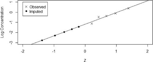
2.5 Method 3: Regression on Order Statistics (ROS) Imputation

Regression on order statistics is a semiparametric method of dealing with censored data and has its origins in environmental statistics. Described by Helsel (2012), it involves replacing the censored values with different values, that is, for a dataset with more than one BLOQ response, different values are imputed onto these multiple responses, as opposed to Methods 1 and 2 which replace all BLOQ values with the same value. To apply this method, we consider each time point in turn, starting with the earliest time point where a BLOQ value is observed. If the error model is multiplicative, transform the data by $c_{ij}=\hspace{0.17em}\text{log}\hspace{0.17em}{y}_{ij}$. The premise of this method is to calculate plotting positions based on quantiles from the Normal distribution for both observed and censored observations, similar to a QQ plot, then using a linear regression to impute values on the BLOQ observations. The method proceeds in detail as follows:

1. Identify BLOQ values.

2. Start at the earliest time point for which a BLOQ value is observed, labeled the jth timepoint. Define n – m as the number of detected responses above or equal to the previously defined LOQ, and m the number of BLOQ values at this time point. From this, we estimate the empirical exceedance probability by the proportion of the sample greater than or equal to the LOQ: $$pe=\frac{n-m}{n}.$$

3. We then calculate the plotting positions for each of the n – m (ordered from lowest to highest) detected values: $$p{d}_j=(1-pe)+\left(\frac{k_d}{n-m+1}\right)pe\hspace{1em}\text{for}\hspace{1em}{k}_d=1,\dots ,n-m.$$

4. We also calculate the plotting positions for each of the m censored BLOQ values: $$p{c}_j=\left(\frac{k_c}{m+1}\right)(1-pe)\hspace{1em}\text{for}\hspace{1em}{k}_c=1,\dots ,m.$$

5. Compute a normal quantile for each value of $p{d}_{k_d}$ and $p{c}_{k_c}$ as $$z_{k_d}^d={\Phi }^{-1}(p{d}_{k_d}),\hspace{1em}{z}_{k_c}^c={\Phi }^{-1}(p{c}_{k_c}).$$

6. Construct a simple linear regression on the $z_{k_d}^d$ and the (ordered from lowest to highest) $y_{k_d}$. $$E(y_{k_d})=\widehat{\alpha }+\widehat{\beta }{z}_{k_d}^d.$$

7. Then we calculate imputed values for the BLOQ values: $$y_{k_c}^c=\widehat{\alpha }+\widehat{\beta }{z}_{k_c}^c.$$

These are ordered by the ordering at the previous timepoint, that is, the highest imputed value is assigned to the subject that has the highest response value on the previous time point.

1. This continues to the next time point until all BLOQ values are imputed.

2. We transform back onto the observation scale if necessary and compute the PK parameter on the augmented data.

Figure 2 shows an example of the application of this method for a single time point. Proceed with NCA methods for AUC estimation using Equations (1)–(4).

Fig. 2 Regression on order statistics example illustrates how imputed values are calculated.

2.6 Method 4: Maximum Likelihood per Timepoint (Summary)

This method does not impute values for the BLOQ observations, but instead provides summary statistics for the concentration at each timepoint under the assumption that each time point is independent. For the jth timepoint, we consider a censored likelihood of $$\begin{array}{c}L({\mu }_j{}^{(A)},{\sigma }_j^{(A)}{}^2)={\left(\Phi \left(\frac{\text{LOQ}-{\mu }_j{}^{(A)}}{{\sigma }_j^{(A)}}\right)\right)}^m\prod _{i=1}^{n-m}\frac{1}{{\sigma }_j^{(A)}\sqrt{2\pi }}\\ \hspace{1em}\times \hspace{0.17em}\text{exp}\hspace{0.17em}\left(\frac{-{(y_{ij}-{\mu }_j{}^{(A)})}^2}{2{\sigma }_j^{(A)}{}^2}\right),\end{array}$$

for the assumption of additive errors, and $$\begin{array}{c}L({\mu }_j{}^{(G)},{\sigma }_j^{(G)}{}^2)={\left(\Phi \left(\frac{\hspace{0.17em}\text{log}\hspace{0.17em}\text{LOQ}-{\mu }_j{}^{(G)}}{{\sigma }_j^{(G)}}\right)\right)}^m\prod _{i=1}^{n-m}\frac{1}{e^{c_{ij}}{\sigma }_j^{(G)}\sqrt{2\pi }}\\ \hspace{1em}\times \hspace{0.17em}\text{exp}\hspace{0.17em}\left(\frac{-{(c_{ij}-{\mu }_j{}^{(G)})}^2}{2{\sigma }_j^{(G)}{}^2}\right),\end{array}$$ for the assumption of multiplicative error. We maximize over μ_j and ${\sigma }_j^2$ to obtain estimates ${\widehat{\mu }}_j$ and ${\widehat{{\sigma }_j}}^2$ for each timepoint t_j. These estimates are then used in the calculation of the point estimate of the AUC and its variance.

2.7 Method 5: Maximum Likelihood per Timepoint (Imputation)

This method is, in essence, a hybrid of Methods 3 and 4. It combines the superior estimation of the mean and variance per time point that censored maximum likelihood brings (Byon, Fletcher, and Brundage 2008), and retains the structure of the between time point relationship that the imputation methods uses. It begins with using maximum likelihood to obtain values of $\widehat{{\mu }_j}$ and $\widehat{{\sigma }_j^2}$ for each timepoint as in Method 4 and subsequently uses these estimates to impute values onto the BLOQ responses using ROS.

2.7.1 Additive Error

Estimate the probability of a response being BLOQ: $$p_{\text{BLOQ}}=P(Y_j<\text{LOQ})=\Phi \left(\frac{\text{LOQ}-{\widehat{\mu }}_j{}^{(A)}}{{\widehat{{\sigma }_j}}^{(A)}}\right),$$ where $\Phi$ is the cumulative distribution function of the standard Normal distribution. We then equally space the probabilities for the censored observations $$p_{k_c}=\frac{k_c}{m+1}{p}_{\text{BLOQ}}\hspace{1em}\text{for}\hspace{1em}3k_c=1,\dots ,m.$$

Transform to response scale using the inverse Normal cumulative distribution function, (${\Phi }^{-1}(·)$). $$y_{k_c}^c={\widehat{\mu }}_j{}^{(A)}+{\widehat{{\sigma }_j}}^{(A)}{\Phi }^{-1}(p_{k_c}).$$

These imputed values are ordered in the same way as in M3 and the PK estimate found on the basis of the imputed dataset.

2.7.2 Multiplicative Error

Estimate the probability of a response being BLOQ: $$p_{\text{BLOQ}}=P(Y_j<\hspace{0.17em}\text{log}\hspace{0.17em}\text{LOQ})=\Phi \left(\frac{\hspace{0.17em}\text{log}\hspace{0.17em}\text{LOQ}-{\widehat{\mu }}_j{}^{(G)}}{{\widehat{{\sigma }_j}}^{(G)}}\right),$$ where F_j is the cumulative distribution function of the Normal distribution with parameters ${\widehat{\mu }}_j{}^{(G)}$ and ${\widehat{\sigma }}_j^{(G)}{}^2$. We then equally space the probabilities for the censored observations $$p_{k_c}=\frac{k_c}{m+1}{p}_{\text{BLOQ}}\hspace{1em}\text{for}\hspace{1em}{k}_c=1,\dots ,m.$$

Transform to response scale using the inverse Normal cumulative distribution function (${\Phi }^{-1}$) and exponentiate. $$y_{k_c}^c=e^{{\widehat{\mu }}_j{}^{(G)}+{\widehat{{\sigma }_j}}^{(G)}{\Phi }^{-1}(p_{k_c})}.$$

These imputed values are ordered in the same way as in M3. Proceed with NCA methods for AUC estimation using Equations (1)–(4).

2.8 Method 6: Full Likelihood

This method takes into account correlation between responses at different timepoints by considering all timepoints together. In this approach, we estimate the covariance matrix of observations assuming a multivariate Normal or Lognormal distribution.

We consider that the data are n independent and identically distributed observations from a ${\text{MVN}}_J(\mathit{\mu },\mathbf{\Sigma })$ distribution. Our objective is to obtain $\widehat{\mathit{\mu }}$ and $\widehat{\mathbf{\Sigma }}$, the maximum likelihood estimates for the mean and variance of the observations assuming a multivariate normal distribution. From these we can then calculate the $\widehat{\text{AUC}}$ and its variance. For each subject $i=1,\dots ,n$, we partition into censored and noncensored observations: $$\begin{array}{c}{\mathit{y}}_{\mathit{i}}^{(\mathit{c})}={\mathit{y}}_{\mathit{i},\{\mathit{j}:{\mathit{\gamma }}_{\mathit{ij}}\mathit{=1}\}},\\ {\mathit{y}}_{\mathit{i}}^{(\mathit{-c})}={\mathit{y}}_{\mathit{i},\{\mathit{j}:{\mathit{\gamma }}_{\mathit{ij}}\mathit{=0}\}},\end{array}$$ where γ_ij is an indicator, taking the value 1 if the observation is censored and 0 otherwise.

We then partition our parameters $\mathit{\mu }$ and $\mathbf{\Sigma }$, with superscripts (c) for censored parameters and $(-c)$ for uncensored, with ${\mathbf{\Sigma }}^{(\mathbf{c})(-\mathbf{c})}$ the censored/uncensored covariance matrix.

Then the conditional (on the uncensored values) distribution of the censored observations following Eaton (1983) is $$\begin{array}{c}\text{MVN}({\mathit{\mu }}^{(\mathit{c})}+{\mathbf{\Sigma }}^{(\mathbf{c})(\mathbf{c})}{({\mathbf{\Sigma }}^{(-\mathbf{c})(-\mathbf{c})})}^{-1}({\mathit{y}}^{(\mathit{-c})}-{\mathit{\mu }}^{(\mathit{-c})}),\\ \hspace{1em}{\mathbf{\Sigma }}^{(\mathbf{c})(\mathbf{c})}-{\mathbf{\Sigma }}^{(\mathbf{c})(-\mathbf{c})}{\mathbf{\Sigma }}^{(-\mathbf{c})(-\mathbf{c})}{}^{-1}{\mathbf{\Sigma }}^{(\mathbf{c})(-\mathbf{c})}{}^T)\end{array}$$ and the log-likelihood can be found as $$\sum _{i=1}^n\left(\hspace{0.17em}\text{log}\hspace{0.17em}\left(F({\mathit{\mu }}^{(c)},{\mathbf{\Sigma }}^{(c)},\text{LOQ})\right)+\hspace{0.17em}\text{log}\hspace{0.17em}\left(f({\mathit{\mu }}^{(-c)},{\Sigma }^{(-c)},{\mathit{y}}_i^{(-c)})\right)\right),$$ where F and f are the cdf and pdf of the multivariate normal distribution, respectively. This is maximized over $\mathit{\mu }$ and $\mathbf{\Sigma }$ to give MLE $\widehat{\mathit{\mu }}$ and $\widehat{\mathbf{\Sigma }}$. The point estimate and variance of the AUC can be estimated from this as follows, with $\mathit{\omega }$ defined as previously in Equations (4)(4) $$\text{var}\left({\widehat{\text{AUC}}}^{(G)}\right)=\sum _{b=1}^B{s}_b^2{}^{(G)},$$(4) and (5)(5) $$s_b^2{}^{(G)}={({\mathit{\omega }}_{\mathit{b}}{e}^{{\overline{\mathit{c}}}_{\mathit{b}}})}^T\widehat{V_b}({\mathit{\omega }}_{\mathit{b}}{e}^{\overline{{\mathit{c}}_{\mathit{b}}}}),$$(5) : $$\begin{array}{c}{\widehat{\text{AUC}}}^{(A)}={\mathit{\omega }}^T\widehat{\mathit{\mu }},\\ \text{var}\left({\widehat{\text{AUC}}}^{(A)}\right)={\mathit{\omega }}^T\widehat{\mathbf{\Sigma }}\mathit{\omega }.\end{array}$$

Similarly, one may construct exactly the same log-likelihood but with the log-normal distribution. Here the parameter estimates $\widehat{\mathit{\mu }}$ and $\widehat{\Sigma }$ represent the mean vector and covariance matrix of the log-transformed data. The point estimate and variance of the AUC can be estimated from this as follows: $$\begin{array}{c}{\widehat{\text{AUC}}}^{(G)}={\mathit{\omega }}^T{e}^{\widehat{\mathit{\mu }}},\\ \text{var}\left({\widehat{\text{AUC}}}^{(G)}\right)={(\mathit{\omega }{e}^{\widehat{\mathit{\mu }}})}^T\widehat{\mathbf{\Sigma }}(\mathit{\omega }{e}^{\widehat{\mathit{\mu }}}).\end{array}$$

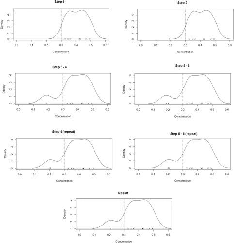
2.9 Method 7: Kernel Density Imputation

This method differs from the previous ones in that it does not assume a specific error distribution, but estimates it from the data. We do still however consider the two cases, using arithmetic (comparable to additive error assumptions) and geometric (comparable to multiplicative error assumptions) means of the responses to estimate the AUC and its variance. The basis of this method uses kernel density estimation (Silverman, 1986), which, given Y_i and a kernel function K, estimates the density of the Y_i as follows: $$\widehat{f}(y)=\frac{1}{nh}\sum _{i=1}^{n}K\left(\frac{y-Y_i}{h}\right),$$ where h is a parameter known as the bandwidth, which can be prespecified or optimized over. In the following, we use a Gaussian Kernel, $K(t)=\frac{1}{\sqrt{2\pi }}{e}^{-(1/2)t^2}$, and use Silverman’s “Rule of Thumb” (Silverman, 1986) to calculate the bandwidth parameter, $h=1.06\widehat{\sigma }{n}^{\frac{1}{5}}$. This h is calculated each time the density $\widehat{f}$ is re-estimated, so that each $\widehat{f}$ has a recalculated bandwidth h. For each timepoint with BLOQ observations, to gain one imputed value:

1. Calculate ${\widehat{f}}_0$ based on uncensored data ${\mathit{y}}^{(-c)}$.

2. Compute $k_0=E_{{\widehat{f}}_0}(Y|Y<\text{LOQ})$.

3. Initialize i = 1.

4. Append $k_{i-1}$ to the uncensored data ${\mathit{y}}^{(-c)}$ and recalculate ${\widehat{f}}_i$.

5. Compute $k_i=E_{{\widehat{f}}_i}(Y|Y<\text{LOQ})$.

6. Let $i=i+1$.

7. Repeat Steps 4–6 until $|k_i-k_{i-1}|<ϵ$ for some very small prespecified value ϵ. This k_i is the value to be imputed.

For a timepoint with m BLOQ values, this process is repeated m – 1 further times to get the m imputed values needed. On each subsequent repetition, the previous imputed value is now appended to the uncensored data. Figure 3 shows an example of the application of this method. Proceed with NCA methods for AUC estimation using Equations (1)–(4).

Fig. 3 A graphical illustration of the KD algorithm. Black circles indicate a new k_i calculated based on the current $\widehat{f_i}$. Gray squares indicate previous k_i values. The dashed line indicates the LOQ.

2.10 Method 8: Discarding BLOQ Values

A final method for consideration is that of simply discarding all responses that are BLOQ, and continuing to use NCA on the remaining data. The point estimate for the $\widehat{\text{AUC}}$ is straightforward to calculate, whether considering additive or multiplicative errors. Although not in the case where all measurements at a given time point are reported BLOQ. However, the variance is not always available in an analytic form as the discarding of BLOQ values results in an unstructured sparse sampling scheme, often where individual sampling times are not repeated. The number of observations is often reduced so much that a jackknife or bootstrap estimate would give inaccurate results.

2.11 Example Application

As an illustration of the eight methods, we apply them to the real example dataset introduced in Section 1.

There is a wide range of values for $\widehat{\text{AUC}}$ and its standard error, all for the same dataset. In both the cases of assumptions of arithmetic and geometric mean, Method 1 unsurprisingly has the lowest $\widehat{\text{AUC}}$. In the case of using geometric means, this is severely lower than all other methods. Method 4 has the lowest variance in each case (apart from the invalid results of Method 6), as expected. When assuming an additive error model, Method 6 failed to produce any results as the assumptions deviated too far from the characteristics of the dataset. When assuming a multiplicative model, although giving results, the optimization was accompanied by a warning regarding the convergence and hence are not viewed as valid results. Method 8, as expected, has the largest $\widehat{\text{AUC}}$ as it has discarded low values. The variance is intractable as some subjects have unique individual sampling times once the BLOQ responses have been discarded.

3 Simulations

To evaluate the performance of the eight methods previously discussed, they are all applied to simulated data. Following an example from Beal (2001), the following model is used to generate data at time t: (6) $$y(t)=C(t)\hspace{0.17em}\text{exp}\hspace{0.17em}(e(t)),$$(6) where C(t) is the PK model and e(t) is the error model. The PK model is a one-compartment IV dose model: (7) $$C(t)=\frac{\text{dose}}{V_d}\text{exp}\hspace{0.17em}(-CL·t),$$(7)

where CL is the clearance, and V_d is the volume of distribution. The error model is Normally distributed $e(t)\sim N(0,h(t))$ with (8) $$h(t)=0.03+0.165\frac{C{(t)}^{-1}}{C{(1.5)}^{-1}+C{(t)}^{-1}}.$$(8)

Data are generated at times $0.5,1,1.5,2,2.5,3$ hr. Two scenarios are considered, using fixed effects and using mixed effects. For fixed effects, the parameters take values $\text{CL}=0.693$, V _d = 1 and $\text{dose}=1$ while for mixed effects, $\text{CL}=\widetilde{\text{CL}}\hspace{0.17em}\text{exp}\hspace{0.17em}({\eta }_1)$ and $V_d=\widetilde{V_d}\hspace{0.17em}\text{exp}\hspace{0.17em}({\eta }_2)$, with $\widetilde{\text{CL}}=0.693,\widetilde{V_d}=1,{\eta }_1\sim N(0,{\omega }_1^2)$ and ${\eta }_2\sim N(0,{\omega }_2^2),\text{corr}({\eta }_1,{\eta }_2)=0$ and ${\omega }_1={\omega }_2=0.2$. 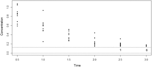An example of such a dataset is illustrated in Figure 4. To explore different levels of censoring, a case with a smaller clearance and dose ($\text{CL}=0.231,\text{dose}=0.25$) is also considered, where the contributions to the AUC will be more affected by how the BLOQ observations are dealt with, illustrated in the motivating example shown earlier in Figure 1. Many more responses are BLOQ for this second example, with one subject having all observed responses BLOQ.

Fig. 4 Illustration of example from Beal (2001), the gray numbers indicate the number of observations that are BLOQ for that time point.

When applying Method 6, we must restrict the dimensionality of the parameter space in order for it to be feasible to realistically used. For example, for this particular set up with six time points considered, there are 27 free parameters to optimize over. This means that optimizing over the multivariate normal log-likelihood takes a very long time and is often unsuccessful or unstable. When performing the maximum likelihood procedure, we therefore now restrict the covariance elements of the matrix for nonconsecutive timepoints to be 0. Hence the variance matrix is tri-diagonal as follows: $$\Sigma =\left(\begin{array}{cccccc}{\text{var}}_1& {\text{cov}}_{12}& 0& 0& 0& 0\\ {\text{cov}}_{12}& {\text{var}}_2& {\text{cov}}_{23}& 0& 0& 0\\ 0& {\text{cov}}_{23}& {\text{var}}_3& {\text{cov}}_{34}& 0& 0\\ 0& 0& {\text{cov}}_{34}& {\text{var}}_4& {\text{cov}}_{45}& 0\\ 0& 0& 0& {\text{cov}}_{45}& {\text{var}}_5& {\text{cov}}_{56}\\ 0& 0& 0& 0& {\text{cov}}_{56}& {\text{var}}_6\end{array}\right)$$

Despite their initial promise stemming from commonly used procedures, in terms of applicability, Methods 1 (replace BLOQ values with 0), 3 (ROS imputation), and 6 (full Likelihood) are not suitable for all datasets and hence are less useful. Method 1 cannot compute any estimates when using geometric means as summaries due to nonfinite values resulting from taking logs. Method 3 requires fitting a linear regression on responses per timepoint and hence is infeasible in scenarios with high levels of censoring that can result in only one response above the LOQ for a given time point. In the simulations, around 1% of the simulated datasets did not result in an estimate. Method 6 is even more unstable, not giving results at all when assumptions on the distribution of the responses is incorrectly specified, and even when the distribution is correctly assumed, up to 3% of simulated datasets do not give results for the fixed effects model and as much as 24% when using mixed effects. For analyzing a single study, the failings of Method 6 are less so, as one may manually tune the optimization. This may however be time consuming and not straightforward. Method 8 is not suitable for many datasets as the variance of the $\widehat{\text{AUC}}$ is intractable due to the sparsity of sampling scheme induced by discarding BLOQ values.

It is desirable for a method to approximate the non-compartmental point estimate and variance of the AUC as closely as possible to that which we would estimate were we to know the true concentration for every response, regardless of a LOQ. Therefore as a measure of performance of the methods in simulations, we use closeness to the full non-compartmental estimates of these values for every simulated dataset, ${\widehat{\text{AUC}}}_{\text{BLOQ}}-{\widehat{\text{AUC}}}_T$ and $\text{var}({\widehat{\text{AUC}}}_{\text{BLOQ}})-\text{var}({\widehat{\text{AUC}}}_T)$, where subscript BLOQ indicates one of the methods of dealing with BLOQ values has been used on the dataset, and subscript T indicates the estimate has been calculated as if we knew all observed values in the dataset, regardless of LOQ.

This criteria of comparison is chosen as opposed to the deviation from the true AUC from the PK model for one principal reason. For a given dataset, the ${\widehat{\text{AUC}}}_T$ as defined previously will by definition, deviate from the underlying true population AUC from the PK model, since it includes variation from the data and is estimated using non-compartmental methods. The non-compartmental methods not only depend on the support points t_j but also on the approximation between observations. However, for any given dataset, this deviation is exactly the same regardless of method of dealing with BLOQ values. Therefore using the deviation of ${\widehat{\text{AUC}}}_{\text{BLOQ}}$ from the true AUC from the PK model is in effect measuring the sum of two deviations, one of which is a constant across methods and therefore unnecessary when the objective is to compare methods. In fact, the added variability between datasets of including this extra deviation may hinder the comparison, since when this composite deviation is compared across all datasets, the two parts cannot be distinguished from one another.

Likewise, one may also consider some “true” non-compartmental estimate of $\widehat{\text{AUC}}$ to compare results to. Although here the dependence on the support points t_j is no longer an issue, the downfall of effectively measuring the sum of two errors mentioned previously still stands. It is of course interest to have some numerical value for bias across methods, and so if of interest to the reader, the appendix in the supplementary materials contains tables giving the bias of each method in varying scenarios using both the trapezoidal and log-trapezoidal rule. The coverage of confidence intervals is also given. Here the “true” value for the $\widehat{\text{AUC}}$ to calculate bias and coverage is obtained by the expectation of the individual $\widehat{\text{AUC}}$ for a given population model. It is worth reiterating that these results are much less relevant from a practical perspective than those presented in the main article, for the reasons discussed previously. For any given dataset, the best approximation to the “true” value for the $\widehat{\text{AUC}}$ is that which is obtained with the full dataset and hence the fairest way to compare methods is a measure of how close they come to this best approximation.

The results for comparison of seven of the eight methods are presented graphically in two ways: boxplots and color plots. Individual simulation results for the variances for Method 8 are not calculable and hence Method 8 (discarding BLOQ values) is not included in the figures. Summary tables of more detailed results for all eight methods can be seen in the appendix in the supplementary materials. Here, the average of variances of the $\widehat{\text{AUC}}$ for Method 8 is approximated by taking the variance of the $\widehat{\text{AUC}}$‘s across the simulated datasets. The performance measures are plotted over 1000 simulations, with standard deviations plotted as opposed to variance for consistency in units. The boxplots (Figures 5 and 6) show the spread of these measures over the simulations. For the most appropriate methods, the color plots (Figure 7) then show the relationship between the deviation from the point estimate and the deviation from the standard deviation over all simulations. The number of simulations has been chosen at 1000 as the more computationally intensive methods, especially Method 6, can take up to 10 min for a single dataset. For 1000 simulations, the coverage of 95% confidence intervals can be classed as simulation error if between 93.65% and 96.35%. In the detailed results in the appendix in the supplementary materials, values outside of this are highlighted.

Fig. 5 Results showing deviation from the non-compartmental $\widehat{\text{AUC}}$, its variance and coverage of confidence intervals with data generated from models with higher dose and clearance. Results over 1000 simulations (10 subjects, 6 timepoints). (F) = Data generated using fixed effects model. (M) = Data generated using mixed effects model. (A) = Analyzed using arithmetic means. (G) = Analyzed using geometric means.

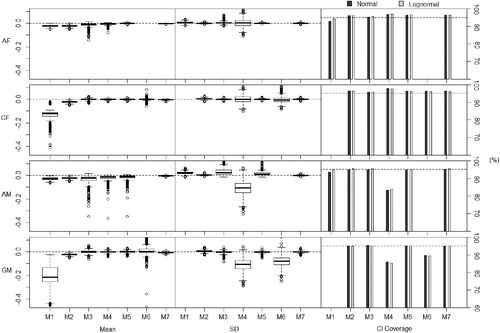
Fig. 6 Results showing deviation from the non-compartmental $\widehat{\text{AUC}}$, its variance and coverage of confidence intervals with data generated from models with lower dose and clearance. Results over 1000 simulations (10 subjects, 6 timepoints). (F) = Data generated using fixed effects model. (M) = Data generated using mixed effects model. (A) = Analyzed using arithmetic means. (G) = Analyzed using geometric means.

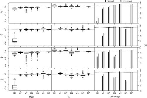
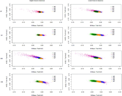
Fig. 7 Results showing deviation from the noncompartmental $\widehat{\text{AUC}}$ and its variance with data generated from both models. Results over 1000 simulations (10 subjects, 6 timepoints). (F) = Data generated using fixed effects model. (M) = Data generated using mixed effects model. (A) = Analyzed using arithmetic means. (G) = Analyzed using geometric means.

For many methods, Figures 5 and 6 show that the estimates of the $\widehat{\text{AUC}}$ underestimates the true non-compartmental estimate. Although Method 5 shows promising performance averaging over the simulations, there is a wider spread over the simulations reaching above and below the truth. For example in the simulations using the mixed effects model with lower dose and clearance analyzed using arithmetic means, the estimate of the $\widehat{\text{AUC}}$ has a standard error of 0.034 using Method 5 but 0.029 using Method 7.

Methods 2 (replace BLOQ values with LOQ/2), 3 (ROS imputation), 5 (maximum likelihood per timepoint (imputation)), and 7 (kernel density imputation) show the most promising results and are therefore compared using the color plots. The color plots in Figure 7 are a clear and direct comparison between the four best performing of eight methods, with Method 7 a clear front runner, as it gives the most consistent results across all simulations and these differences are closest to zero.

As expected, Method 1 underestimates the non-compartmental AUC. One may expect that by imputing the same value onto all BLOQ responses, the estimate of the variance would be underestimated. However, when applied to datasets generated using the mixed effects models, this method overestimates the variance of the $\widehat{\text{AUC}}$. The more the point estimate is underestimated, the more the variance is overestimated. This is because as the imputed values draw the point estimate of the $\widehat{\text{AUC}}$ toward 0, they also increase the deviations of the individual observations from the mean value. These poor estimations lead to poor coverage, especially when applied to the datasets with lower dosage and clearance. This method, as pointed out earlier, is unsuitable when considering the geometric means as methods of summary.

Method 2 shows reasonable results, however, still underestimating the $\widehat{\text{AUC}}$ and overestimating the variance, especially when the data are analyzed using geometric means. This is to be expected as the imputation of LOQ/2 is based on assumptions consistent with analysis using arithmetic means. The coverage of the confidence intervals is noticeably lower than the nominal level when the method is applied to the datasets with lower dosage and clearance.

We see a similar trend as with Method 1 with Method 3 in the case of using arithmetic means, but in an even more extreme way. This method underestimates the $\widehat{\text{AUC}}$ and overestimates the variance even more, especially when the data is generated using the mixed effects model. This method assumes a normal distribution of concentrations per timepoint when analyzing using arithmetic means. This is a significant deviation from the assumptions from the model used in data generation. Although this method performs well for data generated using a fixed effects model and analyzed using geometric means—that is when the assumptions of the method are valid. However, when we deviate from these assumptions, the method performs poorly.

When applied to datasets generated using fixed effects models, Method 4 (maximum likelihood per timepoint (summary)) generally performs well. However, when applied to datasets generated using mixed effects, this method severely underestimates the variance of the $\widehat{\text{AUC}}$. This is because this method assumes independence between timepoints, hence the covariance of responses across timepoints is assumed to be zero. Since these are in fact positively correlated, treating the responses at timepoints as independent will underestimate the variance of the $\widehat{\text{AUC}}$. This gives this method very poor coverage, consistently falling below the nominal level.

Method 5 performs reasonably well when data is generated using the fixed effects model, and using the original parameter values from Beal (2001), even when deviating from assumptions on the distribution of concentrations per timepoint. However, for datasets generated using mixed effects models, this method does not perform as well, underestimating the $\widehat{\text{AUC}}$ and overestimating the variance—with a similar performance for the adjusted model dose and clearance.

Although on a theoretical level Method 6 should perform well, it shows sporadic results. As well as being significantly more computationally intensive than all of the other methods, it does not always give an output and when it does the values are often questionable. Even with the restrictions imposed on the covariance matrix, the high number of free parameters makes the optimization unstable, and when there are deviations from assumptions, the optimization often fails. This method is therefore unsuitable for any realistic use.

Method 7 consistently performs well across all scenarios, with good coverage over all scenarios. The estimates of $\widehat{\text{AUC}}$ and its variance are very close to those which they would be without censoring on BLOQ values. This is because this method does not make assumptions on the distributions, however, does use information from the uncensored observations to impute different values onto the BLOQ responses. It is computationally efficient and can be applied to datasets even with high levels of censoring. We therefore recommend this method as the most appropriate NCA method of dealing with BLOQ responses.

Method 8 performs poorly, consistently overestimating the $\widehat{\text{AUC}}$ due to the omission of all BLOQ values in the NCA, hence inducing a bias. The variance is underestimated, as expected, since the method restricts the range of the responses.

4 Discussion

In this article, we have evaluated the performance of eight different noncompartmental approaches to dealing with observations BLOQ. The simple imputations of Methods 1 and 2, those currently used in practice, are compared to six alternative methods in a number of different scenarios. These scenarios involve the models used by Beal (2001) and also models with lower dose and clearance.

For practical usage, the R package “BLOQ” has been developed and is available on CRAN (Nassiri et al. 2018). This package provides the tools to apply the methods discussed in this article to a given dataset.

The results have shown that the simple imputation methods perform very poorly, especially in scenarios with a large proportion of BLOQ responses. Since these are the methods most commonly used for handling BLOQ values, it is important to note their shortcomings in scenarios that can frequently occur in practice. Methods that use maximum likelihood also fail to estimate the $\widehat{\text{AUC}}$ and its variance well. It is clear that the method of kernel density imputation is the best performing out of all the methods considered and is hence is the preferred method for dealing with BLOQ responses in NCA.

The limitations of the method include the issue from which all methods apart from simple imputation of a single value suffer—the scenario where all responses at a given time point are reported as BLOQ. In this case, since the only information on responses at that time point is that they all lie between 0 and LOQ, nothing is known about the distribution of the responses and hence no kernel density estimation can be calculated. There is also the scope to improve the method further by considering alternative kernels to the one we have implemented.

Although in this article, we have only looked at studies that have full sampling schemes, the kernel density imputation method can easily be applied to sparse sampling schemes. The imputation values are calculated in exactly the same way, it is only the process of ordering of these values that will differ.

For serial sampling, where one blood sample is taken per subject, the ordering at any given time point is of no concern and hence can be assigned randomly. In batch designs, the ordering can be based on the previous time point that the specific batch was sampled at, instead of the previous time point. For more flexible designs, the subjects are not separated into disjoint batches by their time points, but for each individual set of sampling times, there must be at least two subjects following this in order for the variance of the non-compartmental estimate of the $\widehat{\text{AUC}}$ to be calculated. If all subjects with BLOQ responses are on the same set of sampling times, the ordering will be based on the responses at previous time point from those sampling times. If all subjects are not on the same set of sampling times then one may choose the allocation will be random or by some other rule, for example, one based on gradients of linear interpolations between responses at different time points.

This method is by no means limited to PK studies. It can also be further extended to other scenarios where left-censored values are present but no model fitting takes place. The scope of the application of kernel density imputation is wide, and the potential to extend to further more complicated settings is promising.

Supplementary Materials

The Supplementary Materials contain an Appendix with tables of detailed results from additional simulations.

Additional information

Funding

We gratefully acknowledge the funding and support of the EPSRC funded EP/H023151/1 STOR-i centre for doctoral training and Janssen Pharmaceutica. Prof. Jaki’s contribution to this report is independent research supported by the National Institute for Health Research (NIHR Senior Research Fellowship, Dr. Thomas Jaki, SRF-2015-08-001). The views expressed in this publication are those of the author(s) and not necessarily those of the NHS, the National Institute for Health Research, or the Department of Health.

References

- Armbruster, D. A., and Pry, T. (2008), “Limit of Blank, Limit of Detection and Limit of Quantitation,” The Clinical Biochemist Reviews, 29, 49–52.
- Barnett, H. Y., Geys, H., Jacobs, T., and Jaki, T. (2018), “Optimal Designs for Non-Compartmental Analysis of Pharmacokinetic Studies,” Statistics in Biopharmaceutical Research, 10, 255–263. DOI: 10.1080/19466315.2018.1458647.
- Beal, S. L. (2001), “Ways to Fit a PK Model With Some Data Below the Quantification Limit,” Journal of Pharmacokinetics and Pharmacodynamics, 28, 481–504.
- Bonate, P. L. (2006), Pharmacokinetic-Pharmacodynamic Modeling and Simulation, New York: Springer.
- Byon, W., Fletcher, C. V., and Brundage, R. C. (2008), “Impact of Censoring Data Below an Arbitrary Quantification Limit on Structural Model Misspecification,” Journal of Pharmacokinetics and Pharmacodynamics, 35, 101–116. DOI: 10.1007/s10928-007-9078-9.
- Cawello, W. (2003), Parameters for Compartment-free Pharmacokinetics—Standardisation of Study Design, Data Analysis and Reporting, Aachen: Shaker Verlag.
- Chapman, K., Chivers, S., Gliddon, D., Mitchell, D., Robinson, S., Sangster, T., Sparrow, S., Spooner, N., and Wilson, A. (2014), “Overcoming the Barriers to the Uptake of Nonclinical Microsampling in Regulatory Safety Studies,” Drug Discovery Today, 19, 528–532. DOI: 10.1016/j.drudis.2014.01.002.
- Davidian, M., and Giltinan, D. M. (1995), “Nonlinear Models for Repeated Measurement Data, Boca Raton, FL: Chapman & Hall/CRC.
- Dykstra, K., Mehrotra, N., Tornøe, C. W., Kastrissios, H., Patel, B., Al-Huniti, N., Jadhav, P., Wang, Y., and Byon, W. (2015), “Reporting Guidelines for Population Pharmacokinetic Analyses,” Journal of Pharmacokinetics and Pharmacodynamics, 42, 301–314. DOI: 10.1007/s10928-015-9417-1.
- Eaton, M. L. (1983), “The Normal Distribution on a Vector Space,” in Multivariate Statistics: A Vector Space Approach, ed. R. A. Vitale, New York: Wiley, Chapter 3, pp. 116–117.
- Gabrielsson, J., and Weiner, D. (2001), Pharmacokinetic and Pharmacodynamic Data Analysis: Concepts and Applications (Vol. 1), Boca Raton, FL: CRC Press.
- Gagnon, R. C., and Peterson, J. J. (1998), “Estimation of Confidence Intervals for Area Under the Curve From Destructively Obtained Pharmacokinetic Data,” Journal of Pharmacokinetics and Biopharmaceutics, 26, 87–102.
- Gibaldi, M., and Perrier, D. (1982), Pharmacokinetics, New York: Marcel Dekker.
- Helsel, D. R. (2012), Statistics for Censored Environmental Data Using Minitab and R (2nd ed.), Hoboken, NJ: Wiley.
- Hing, J. P., Woolfrey, S. G., Greenslade, D., and Wright, P. M. C. (2001), “Analysis of Toxicokinetic Data Using NONMEM: Impact of Quantification Limit and Replacement Strategies for Censored Data,” Journal of Pharmacokinetics and Pharmacodynamics, 28, 465–479.
- Jaki, T., and Wolfsegger, M. J. (2012), “Non-Compartmental Estimation of Pharmacokinetic Parameters for Flexible Sampling Designs,” Statistics in Medicine, 31, 1059–1073. DOI: 10.1002/sim.4386.
- Johnson, J. R. (2018), “Methods for Handling Concentration Values Below the Limit of Quantification in PK Studies,” in PhUSE US Connect 2018, pp. 1–9.
- Little, R. J. A., and Rubin, D. B. (2002), Statistical Analysis With Missing Data (2nd ed.), Hoboken, NJ: Wiley.
- Nassiri, V., Barnett, H., Geys, H., Jacobs, T., and Jaki, T. (2018), “BLOQ: Impute and Analyze Data With Observations Below the Limit of Quantification,” available at https://cran.r-project.org/web/packages/BLOQ/.
- Reisfield, B., and Mayeno, A. N. (eds.) (2013), Computational Toxicology (Vol. 1), Totowa, NJ: Springer.
- Rubin, D. B. (1987), Multiple Imputation for Nonresponse in Surveys, New York: Wiley.
- Silverman, B. W. (1986), Density Estimation for Statistics and Data Analysis, London: Chapman & Hall.
- Wang, Y. (2015), “For the Release of Bioanalytical Data Below the LLOQ. A Presentation Entitled Evolution of Pharmacokinetics at FDA in the Last Decade,” available at http://zerista.s3.amazonaws.com/item_files/0f21/attachments/58920/original/170.pdf.