The Use of a Variable Representing Compliance Improves Accuracy of Estimation of the Effect of Treatment Allocation Regardless of Discontinuation in Trials with Incomplete Follow-up

Abstract

Abstract–In Clinical Trials, not all randomized patients follow the course of treatment they are allocated to. The potential impact of such deviations is increasingly recognized, and it has been one of the reasons for a redefinition of the targets of estimation (“Estimands”) in the ICH E9 draft Addendum. Among others, the effect of treatment assignment, regardless of the adherence, appears an Estimand of practical interest, in line with the intention-to-treat principle. This study aims at evaluating the performance of different estimation techniques in trials with incomplete post-discontinuation follow-up when a “treatment-policy” strategy is implemented. To achieve that, we have (i) modeled and visualized as directed acyclic diagram a reasonable data-generating model; (ii) investigated which set of variables allows identification and estimation of such effect; (iii) simulated 10,000 trials in Major Depressive Disorder, with varying real treatment effects, proportions of patients discontinuing the treatment, and incomplete follow-up. Our results suggest that, at least in a “Missing at Random” setting, all studied estimation methods increase their performance when a variable representing compliance is used. This effect is more pronounced the higher the proportion of post-discontinuation follow-up is.

KEYWORDS:

• Compliance
• Estimands
• Treatment discontinuation
• Treatment policy

1 Introduction

It has long been known that randomized clinical trials (RCTs) are imperfect experiments. Patients do not always comply with the treatment course they are assigned to. Due to adverse events, to a perceived lack of improvement, or to a combination of the two, patients might decide to discontinue their treatment. Sometimes investigators themselves might need to advise patients to do so for the same reasons.

Historically, non-outcome events that occur during a trial have been mostly discussed for their potential to lead to data missingness of the outcome variable or of other variables of interest. The description of missingness mechanisms refers to terms introduced by Rubin (1976). We summarize here their interpretation based on conditional independencies, widely reported (e.g., Schafer and Graham 2002; National Research Council 2010):

• Values for a variable Y are Missing Completely at Random (MCAR) if the probability of its missingness (RY) is independent of all observed data (X, i.e., one or more observed variables) and of the missing or partially observed (Ymis) itself:(1) $$p\left(RY\right)\perp \mathrm{}\mathrm{}\perp X,\mathit{Ymis}.$$(1)

• Values are missing at random (MAR) if missingness is independent on the missing or partially observed data conditionally on observed data.(2) $$p\left(RY\right)\perp \mathrm{}\mathrm{}\perp \mathit{Ymis}|X.$$(2)

• Values are missing not at random (MNAR) if missingness depends on the missing or partially observed data and no set of observed variables exists that satisfies (2).

The Estimand framework (International Council on Harmonization of Technical Requirements for Registration of Pharmaceuticals for Human Use 2019), explicitly acknowledges the impact on the question that the study answers of the choices made to deal with the events that “occur after treatment initiation and either preclude the observation of the [endpoint] variable or affect its interpretation” (hereinafter referred to as “intercurrent events”). Strategies for handling intercurrent events include:

• Treatment policy where the target of estimation is considered regardless of the occurrence of the intercurrent event (in line with the Intention-To-Treat principle).

• Composite where the intercurrent event is made a component of the variable (e.g., integrated in the definition of a composite endpoints of treatment failure or success).

• Hypothetical where the target of estimation refers to a hypothetical scenario where the intercurrent event would not have occurred.

• While-on-treatment where the timeframe of interest for the outcome is defined by the occurrence of the intercurrent event.

• Principal stratum where the target population is selected based on the occurrence (or nonoccurrence) of the intercurrent event both under the observed and unobserved assignments (e.g., patients who would not discontinue neither the investigational treatment nor the placebo).

The Estimand framework reframes the problem of missing data in clinical trials. Research on methods of estimations—including the treatment of missing data—in relation with the requirements of this new framework is only recently growing. The framework has certainly given the vocabulary and context to discuss whether and how analysis methods shape the question of interest (Permutt 2019, 2020).

Despite its recent adoption, the framework has been already included in guidance that the EMA issues to developers (for example in EMA, 2018a, 2018b, 2018c), confirming its relevance for regulatory decision-making. In this article, we discuss estimation in the following situation: the estimand of interest adopts a treatment-policy strategy for treatment discontinuation, the outcome is a nonbinary quantity measured repeatedly, the treatment can be discontinued at different timepoints, and some patients (but not all) are followed-up after treatment discontinuation.

In Section 2, we will first present and justify the estimand for which we will then test different possible estimators.

Following that, we will present the data-generating mechanism, including assumptions that can generally be made regarding the missingness mechanism in case of noncompliance. Furthermore, we will present the simulation experiment implementing the data-generating mechanism described and in Section 2.4, the estimators tested and the performance indicators used.

In Section 3, we will focus on the performance of the estimators tested given the scenarios described in Section 2, and we demonstrate that both available post-baseline measurements of the outcome and a compliance indicator should be taken into account in the analysis in presence of noncompliance, treatment effect, and missingness.

Furthermore, we will explore and discuss in Section 4 how the performance of such estimators changes depending on certain characteristics of the data.

2 Methods

2.1 High Level Presentation of the Context and Definition of the Estimand

We will here consider the case of trials in Major Depressive Disorder (MDD), comparing an investigational treatment with placebo at six weeks using the 17-item Hamilton Depression Scale (Hamilton 1960) (HAM17) as a primary endpoint. In addition to baseline ($t_0)$ and six weeks ($t_3)$, the state of the patients is also simulated at two ($t_1)$ and four weeks ($t_2)$.

To isolate the effect of different ways of handling treatment discontinuation, we will here limit the discussion to the handling of such one intercurrent event. In line with the ICH E9 Addendum (ICH 2019), the Estimand is described as follows:

1. Treatment condition of interest: assigned to treatment with an experimental antidepressant, regardless of compliance; alternative treatment condition: assigned to placebo.

2. Population: patients diagnosed with MDD and a baseline severity of at least 20 points on the HAM17.

3. Variable: change from baseline of the HAM17 score at six weeks.

4. Population-level summary: difference in variable means between treatment assignments.

This strategy to deal with treatment discontinuation is described in the ICH E9 Addendum as “treatment-policy.” In other words, we acknowledge that our estimand is—in line with the ITT principle—the effect of the decision to treat a patient rather than the effect of treatment. To be clear, this does not imply nor assume the existence of any direct effect of assignment (i.e., it is compatible with the treatment administration mediating fully the effect of treatment assignment).

2.2 Representation of the Data-Generating Mechanism

Following the approach proposed by Mohan, Pearl, and Tian (2013) and Mohan and Pearl (2019), we use a causal diagram (Pearl 1995) to provide a transparent representation of the assumptions regarding the data-generating mechanism, including the mechanism leading to data missingness, and to encode information regarding conditional independence. The missingness graph (m-graph) representing the structure of the data-generating mechanism that we will consider in this work for any timepoint T is shown in Figure 1, assuming that the treatment has an effect on the outcome in at least some of the patients. This is not meant to substitute, but rather to complement and inform, Rubin’s classification of the missingness mechanisms described above.

Fig. 1 The data-generating mechanism if treatment can affect the outcome, represented according to Mohan, Pearl, and Tian (2013). Each directed line represents a causal relationship from a variable to another. Z = random assignment; X_t = whether the patient complies with the treatment at time t; RY_t = the response indicator at time t; Y_t= the real value of HAM17 in a patient at time t; Y_t* = the observed HAM17 value at time t. See text for details.

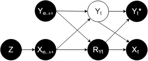
Z is the (randomized) assignment. It has no causes by design, and it is a cause of the exposure to treatment ($X_t)$, starting with the exposure to treatment between t₀ and t₁ ($X_{t0})$. When 0, it assigns patients to placebo ($X_{t0}=0$), when 1, it assigns to patients to active treatment ($X_{t0}=1$).

For any time-point t (e.g., for t₃, the time-point used for the primary measurement of outcome), the node Y_t, represented in white, is the true value of HAM17 at time t, while Y_t* is the observed value of HAM17 at time t.

RY_t is the response indicator, if it takes the value “1”, Y_t is observed and Y_t* exists and it is equal to Y_t, otherwise (i.e., if RY_t is 0) Y_t* is missing and Y_t is unobserved.

For any t, $Y_{t0,\dots ,t-1}$ are the values of HAM17 at all time-points before t. For example, for t = 3, $Y_{t0,\dots ,t-1}$ are {$Y_{t0}$; $Y_{t1}$; $Y_{t2}$}.

At each time-point after t₀, a patient assigned to the active treatment can continue or discontinue the treatment. This decision is represented by the binary variable X_t taking value of 1 if the treatment was continued and 0 if it was discontinued. Hence, for any t, $X_{t0,\dots ,t-1}$ describes the exposure to treatment between t₀ and t. For example, for a patient who discontinued treatment at t₂ (i.e., received treatment up to t₂, but not between t₂ and $t_3),X_{t0,\dots ,t-1}$ will be {$X_{t0}=1$; $X_{t1}=1$; $X_{t2}=0$}.

With the understanding that patients assigned to placebo will not be exposed to drug (i.e., $X_{t0}=X_{t1}=X_{t2}=0$), X_t represents—for the patients assigned to active treatment—the observed compliance.

The representation of compliance between two visits as a binary variable corresponds to the case for treatments that are administered in the clinic and for which the effect is postulated to happen (or last) between visits, and by approximation in cases where the treatment is made available to the patients at each visit and taken by the patient independently. A more granular analysis of the latter scenario might consider exposure to treatment between visits as a partially observed binary or discrete covariate, but this will be omitted here for simplicity.

Each directed arrow present or absent in Figure 1 encodes a causal assumption. Importantly, we assume that (i) HAM17 at any given time-point ($Y_t)$ depends on all previous values of HAM17 ($Y_{t0,\dots ,t-1})$ and all previous treatment exposures ($X_{t0,\dots ,t-1})$; (ii) whether or not the value of HAM17 at any given time-point is available (RY ${}_t)$ is dependent on all previous values of HAM17 ($Y_{t0,\dots ,t-1})$ and all previous treatment exposures ($X_{t0,\dots ,t-1})$, but not on the current HAM17 $(Y_t)$.

It is possible to identify by d-separation (Pearl and Paz 1985) in the m-graph the set of variables—if one exists—that would make the probability of missingness (RY ${}_t)$ independent (i.e., not connected by a “path” in the diagram) from the partially observed value Y_t. For that purpose, we consider the undirected paths that might connect the two variables:

• {RY ${}_t\to X_{t+1}\leftarrow Y_t$} is blocked by $X_{t+1}$ as arrows point in its direction on both sides (i.e., it is a “collider”).

• {RY ${}_t\to Y_{t\ast }\leftarrow Y_t$} is blocked by $Y_{t\ast }$, also a collider.

• {RY ${}_t\leftarrow X_{t0,\dots ,t-1}\to Y_t$} can be blocked by conditioning for $X_{t0,\dots ,t-1}$.

• {RY ${}_t\leftarrow Y_{t0,\dots ,t-1}\to Y_t$} can be blocked by conditioning for $Y_{t0,\dots ,t-1}$.

The conditional independences identified can be written as(3) $$p\left(R{Y}_t\right)\perp \mathrm{}\mathrm{}\perp Y_t|X_{t0,\dots ,t-1},Y_{t0,\dots ,t-1}.$$(3)

As (3) is an instance of (2), we can conclude that the missingness mechanism described is MAR, provided we condition on values of HAM17 and exposure to treatment at all previous time-points.

Figure 1 does not contain a directed arrow from Y_t to RY_t. This assumes that the true value of HAM17 does not cause its missingness. To be clear, the figure does encode an association between HAM17 and its missingness, but this association is assumed to be explained by HAM17 at previous timepoints and previous exposure to treatment.

A missingness mechanism in which Y_t causes RY_t (corresponding to MNAR) is arguably equally plausible and should be explored in sensitivity analyses. It is outside the scope of this article where we focus on central estimation of identifiable quantities.

Figure 1 is elaborated assuming that the treatment has the potential to influence outcome in at least some of the patients. To study estimation under the absence of treatment effect, we have also encoded the assumptions in a scenario when this causal relationship is absent (Figure 2).

Fig. 2 The data-generating mechanism if treatment never affects outcome, represented according to Mohan, Pearl, and Tian (2013). Each directed line represents a causal relationship from a variable to another. Z = random assignment; X_t = whether the patient complies with the treatment at time t; RY_t = the response indicator at time t; Y_t= the real value of HAM17 in a patient at time t; Y_t* = the observed HAM17 value at time t. See text for details.

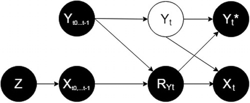
Figure 2 differs from Figure 1 only by the absence of a directed arrow between $X_{t0,\dots ,t-1}$ and Y_t. This erases the path $R{Y}_t\leftarrow X_{t0,\dots ,t-1}\to Y_t$ and the need of conditioning for $X_{t0,\dots ,t-1}$. However, conditioning for $X_{t0,\dots ,t-1}$ in this scenario does not create new (biasing) paths between RY_t and Y_t (only conditioning on colliders open new paths, and $X_{t0,\dots ,t-1}$ does not become a collider in Figure 2). Hence, it is not expected to bias estimation.

2.3 Simulation Overview

We developed a simulation of a clinical trial in MDD, with three timepoints—including baseline—where the treatment is given to patients and four—including baseline and endpoint—where the HAM17 score is recorded.

To explore the performance of the estimators in a wide range of scenarios, we have allowed several parameters to vary, as described below and in Table 1. An alternative could have been to generate separate sets of simulations for different (but fixed within sets) values of—for example—treatment effect and proportion of missingness. However, the approach we followed provides greater flexibility when the effect of different parameters is of interest. However, given that the performance under the null hypothesis of no treatment effect is considered a distinct question, we have generated separate sets of stimulations in presence and in absence of treatment effect (see below).

Table 1 Some of the parameters allowed to vary at each simulated trial and their allowed range.

Parameter	Allowed range (uniform distribution)
Sample size (per arm)	150–250
Mean drug effect between t0 and t1	0.01–0.3
Mean drug effect between t1 and t2	Mean drug effect between t0 and t1 to 0.8
Mean drug effect between t2 and t3	Mean drug effect between t1 and t2 to 1.5
% of delayed effect	0.01–0.15
Treatment discontinuation probability (per visit) for patients performing better than average	0.15–0.45
Treatment discontinuation probability (per visit) for patients performing worse than average	Rate for the ones performing better to 0.6
Post-discontinuation retention probability for patients performing worse than average	0.25–0.5
Post-discontinuation retention probability for patients performing better than average	Rate for the ones performing worse to 0.6

At each of the iterations, we start by defining a sample size (a random even number between 300 and 500) and simulating an investigational treatment and a population (five times the sample size).

The investigational treatment is allowed to assume different level of efficacy for each interval (i.e., between t₀ and t₁, t₁ and t₂, and t₂ and $t_3)$.

The population is simulated assigning to each individual a baseline HAM17 score—normally distributed with mean 20 and standard deviation (SD) 5, and responsiveness to treatment between -0.5 and 2.5, with mean 1 and SD 1. This individual responsiveness should be interpreted as the (generally unmeasured) characteristics that identify patients that respond better, or worse, to a given treatment. In practice it is a modifier of each patient’s response to treatment, as it multiplies for each patient receiving the investigational treatment between each two time-points the randomly generated (average) drug effect. It is considered unknown and it is only used for data generation, as it is not included in any of the imputation and analysis models. From the simulated population a number of individuals equal to the sample size randomly chosen between 300 and 500 with $\text{HAM}17\ge 20$ are selected and assigned to active treatment or placebo in a 1:1 ratio. At each subsequent timepoints t_x, we allowed the HAM17 score to depend on baseline score, exposures to treatment from t₀ to t_x, responsiveness, random natural fluctuation (between -5 and +5) and measurement error. The heterogeneity of responsiveness and disease courses has been included in the data-generating model in order to avoid that unrealistically uniform data could influence the conclusions on the performance of the estimators.

Treatment discontinuations and interruption of follow-up were implemented according to the data-generating mechanism described in the previous chapter (see Appendix I in the supplementary materials for details).

We allowed the intercurrent event of treatment discontinuation to occur at t₁ and t₂ and—after treatment discontinuation—we allowed patients to continue or interrupt follow-up (i.e., to be missing at t₂ and $t_3)$. To better isolate the effects of handling treatment discontinuation, we did not simulate other intercurrent events and we did not allow missing data in the control arm or for other reasons (including before discontinuation, hence there is no missing data at $t_0)$. Both treatment discontinuation at t_x ($X_t)$ and interruption of follow-up at $t_{x+1}$ (RY ${}_{t+1})$ were set to be more likely in patients performing relatively worse (i.e., with a higher $Y_t)$. The latter means data were MAR and not MNAR by design. Parameters on treatment discontinuation and retention after discontinuation were allowed to vary (see Table 1), but the monotone pattern (see Figure S1) was built into the simulation and always assumed. In other words, we assumed both that patients who discontinue treatment do not resume it and that patients who discontinue follow-up do not resume it.

2.4 Evaluation of Different Estimators

Under both the data-generating mechanisms described in Figures 1 and 2 (i.e., in presence and absence of a treatment effect), 10,000 simulations have been performed in R 3.5.1 (R Core Team 2018).

Owing to the nature of this simulation experiment—and unlike in practice—the real value of the estimand has been measured exactly before implementing data missingness. This has been done in line with the definition of treatment-policy (ICH 2019) whereby data should be used regardless the occurrence of the intercurrent event. Hence, estimation is straightforward in case of absence of missing data, which we obtain by simulating data before simulating their missingness.

The performance of different methods in different configurations (as described below) was then characterized through the following performance measures (van Buuren 2012):

• Bias, defined as the average difference between the real value for the estimand in the sample and its estimate. Given the nature of our simulation experiment, this is a measure of bias due to missingness, conditional on sample.

• Coverage, defined as the % of times when the real value for the estimand in the sample falls within the 95% confidence interval (CI) for its estimate.

• Length of 95%CI.

In addition, we report the mean squared error (MSE), calculated as the square of the difference between the real and the estimated values of the estimand in the sample. We considered bias, coverage and MSE as measures of accuracy, and length of 95% CI as a measure of precision.

In introducing the methods below, we point out that the alignment between an estimand and an estimator critically depends on the assumptions we are ready to make regarding the data-generating mechanism. In line with this principle, we will discuss which set of assumptions makes each of the estimators suited to the treatment-policy strategy chosen.

2.4.1 Static Methods

To provide context for the evaluation of the performance of the methods under investigation, estimations using two simple methods have been reported.

As an extreme example, we used a complete-case analysis (i.e., we only included in the analysis complete cases, ignoring incomplete cases). This method is known to produce biased estimates if the missingness mechanism is different than MAR (Baraldi and Enders 2010), so that patients who have complete data are an unbiased representation of the whole sample. Given our setting and our estimand, this would require(4) $$p\left(R_Y\right)\perp \mathrm{}\mathrm{}\perp Z,Y_{t0,\dots ,t-1},X_{t0,\dots ,t-1},X{Y}_{\mathit{tmis}}.$$(4)

Which is of course an instance of (1) and not the case in our simulations and in most realistic scenarios. In particular, for our estimand, this method would lead to an overestimation of the effect where there is a treatment effect and patients have to comply with the treatment to benefit from it (as it is in our simulations generated according to Figure 1), or at least where—even in absence of a treatment effect—patients who are missing in the treatment arm are worse than the ones who are not missing by a greater difference than in the control arm. This could be the case for example when patients who perform worse more easily drop out from a trial when assigned to an active and potentially toxic treatment, and it is the case in our simulations.

As a method that does take into account difference between patients, we investigated a simple mixed-effects model where patients are included as random effects, and the interaction between treatment assignment and time as fixed effect. In this configuration, the effect of treatment would be estimated using all available data without accounting in any way for the compliance. In other words, given the setting and the estimand chosen, it would only be an appropriate estimator if, given the baseline and post-baseline severity measures, the missing values would be independent from their missingness. More formally, it requires:(5) $$p\left(R{Y}_t\right)\perp \mathrm{}\mathrm{}\perp Y_t|Y_{t0,\dots ,t-1}.$$(5)

This is obviously an instance of MAR (2) but more restrictive than (3) as it does not account for compliance and it is not the case in the simulations performed according to Figure 1 and in most setting where a treatment has an effect and patients have to comply with the treatment in order to benefit from it. Additionally, the way the subject is specified as random effect would in essence account for the prognosis in patients assigned to placebo and for prognosis and responsiveness to treatment in the patients assigned to active treatment, but would be erroneous/meaningless for patients that contribute with both on-treatment and off-treatment data. Maximum likelihood estimation methods are explored in more detail below with auxiliary variables (see below).

2.4.2 Methods Under Investigation

We have investigated the performance of methods of multiple imputations, maximum-likelihood, and weighting-based approaches in different configurations, that is, accounting for the following covariates:

1. Baseline severity ($Y_0)$ only. This is would be expected to account adequately for missingness in case:(6) $$p\left(R{Y}_t\right)\perp \mathrm{}\mathrm{}\perp Y_t|Y_{t0},$$(6)

   which is not by design the case in our simulations (both in presence and in absence of a treatment effect). Arguably, and even extending this configuration to include other measured baseline variables, it is unlikely they account for missingness in a satisfactory manner in any realistic scenario.

2. Baseline and post-baseline severity ($Y_{t0,\dots ,t-1})$. This would be expected to give unbiased results in case (5) were satisfied. This is the case by design in our simulations in absence, but not in presence of a treatment effect. In other words, this would require that both the intercurrent event and the missingness be noninformative.

3. Baseline and post-baseline severity ($Y_{t0,\dots ,t-1})$ and a compliance indicator ($X_{t0,\dots ,t-1})$. This is expected to allow unbiased estimates under (3), a permissive definition of MAR which is true in our simulation and credible in realistic scenarios. In other words, this requires that the missingness be non-informative, but allows for the intercurrent event to be informative.

It is worth emphasizing that our aim was to evaluate how the proper specification of the covariates would improve the performance of each of the methods, thus the comparison of conceptually different methods was outside the scope of this article.

Multiple Imputation Methods

We used three multiple imputation methods for which we included observed compliance and observed disease severity at all previous timepoints in the prediction matrix, they are briefly described below.

• For the predictive mean matching (PMM), a regression is built based on all complete cases. This regression is then applied to predict the outcome on the whole sample (including complete cases) in order to identify which ones of the complete cases have predicted values closer to the predicted values of incomplete cases. The actual outcome value for one of the closest 5 potential “donors” is taken to replace each missing value in each copy of the dataset (Rubin 1986; Little 1988).

• A classification and regression “tree” (CART) (Breiman et al. 1984) is built on the complete data by recursive partitioning. Each case with missing outcome is then put down the tree and the value from a neighbor on the same “leaf” is randomly taken as a replacement (Doove, van Buuren, and Dusseldorp 2014).

• The Schafer’s linear regression imputation (NORM) (Rubin 1987; Schafer 1997) defines an additive linear regression model with no interaction terms assuming normal distribution and imputes adding residual noise.

All imputation methods have been performed on five copies of the dataset and the pooling of the analysis results has been performed according to Rubin (1987), as implemented in the R package MICE (van Buuren 2018).

Given the monotone pattern of missingness (see Figure 2), imputation methods have been employed with sequential imputation (i.e., $Y_{t2}$ was imputed first on all cases, and then $Y_{t3}$ was imputed).

The covariates accounted for in the different configurations (see above) have been included in the imputation model.

Maximum Likelihood Methods

We applied the full information maximum likelihood approach (Finkbeiner 1979) as implemented in the R package lavaan (Rosseel 2012)—a method for the estimation of parameters without imputation but using all available data.

The covariates accounted for in the different configurations (see above) have been added as auxiliary variables (Enders 2008).

Weighting-Based Approaches

As complete case analysis is expected to bias results when the probability of missingness is associated with the outcome of interest, a conceptually appealing approach is weighting complete cases by the inverse of their probability of being complete (Seaman and White 2013).

For the inverse probability weighting approach, we have derived the weights from the baseline values only, then from all available HAM17 values, and then from the whole set of predictors in (3) including compliance indicator. The problem of calculating the weights in presence of a partially observed predictor has been solved in two different ways:

• In the model using all post-baseline observation of the HAM17 but not the observed compliance, a single imputation based on the normal distribution with the previous observations as predictor has been used.

• In the model using all post-baseline observations of the HAM17 and compliance, the following decomposition was applied:(7) $$\begin{array}{c}p\left(R{Y}_3\right)|X_{t0,\dots ,t-1},Y_{t0,\dots ,t-1}=\\ p\left(R{Y}_2\right)\left|X_{t0,\dots ,t-1},Y_{t0,\dots ,t-1}xp\left(RY3\right)\right|RY2\\ \hspace{1em}=1,X_{t0,\dots ,t-1},Y_{t0,\dots ,t-1}.\end{array}$$(7)

The two probabilities on the right-hand side were estimated separately and then the probability on the left-hand side was calculated and used for the inverse weights. Given monotonicity of the missing data pattern (see Figure S1), (4) did not require the use of any missing data (for all patients with missing data at t₂, the probability of missing data at t₃ was 1, and did not require the missing value to be calculated).

Weights have been estimated from a logistic regression, stabilized by the probability of being missing in the whole sample, and extreme weights (i.e., the top and bottom 2.5%) have been trimmed (Potter 1993).

3 Results

In total, 10,000 simulations have been produced under a range of nonzero underlying treatment effects. The simulations had a median true effect of the estimand in the sample across simulations of –0.89 (IQ –41.28 to –0.5), a median proportion of missingness in the outcome at t₃ of 22.36% (IQ 18.82%–25.2%), a median proportion of patients discontinuing treatment of 38% (minimum 15%, maximum 52%) and a median sample size of 398 (IQ 348–448).

On the 10,000 simulations with no underlying treatment effect, median true effect of the estimand in the sample across simulations was 0 (IQ –0.32 to 0.33), the median proportion of missingness in the outcome at t₃ is 22.23% (IQ 19%–25.25%), a median proportion of patients discontinuing treatment of 38% (minimum 15%, maximum 52%), and the median sample size is 398 (IQ 349.5–448).

In both simulations sets, missingness pattern was always monotone, as shown in Figure S1. Tables 2 and 3 show—respectively, for the simulations run with and without an effect of treatment on outcome—bias, coverage, and length of the confidence interval for the estimation methods described above.

Table 2 Bias, coverage, length of the 95%CI, and mean squared error (MSE) for the 10,000 simulations performed under the existence of a treatment effect.

Method	Bias (SE)	Coverage (%)	CI length	MSE
Complete case analysis	–1.026 (0.005)	63.91	2.356	1.315
Mixed effects model	–0.606 (0.002)	75.22	1.589	0.451
				NORM
Baseline imputation model	–0.701 (0.003)	86.85	2.245	0.629
+ other HAM17 values	–0.398 (0.002)	99.37	2.112	0.216
+ compliance	–0.004 (0.01)	99.8	2.33	0.094
				PMM
Baseline imputation model	–0.697 (0.004)	86.87	2.255	0.629
+ other HAM17 values	–0.401 (0.002)	99.29	2.1	0.219
+ compliance	–0.013 (0.003)	99.89	2.314	0.096
				CART
Baseline imputation model	–0.676 (0.004)	83.38	2.1	0.602
+ other HAM17 values	–0.343 (0.002)	99.44	2.048	0.175
+ compliance	–0.198 (0.002)	99.877	2.043	0.096
				FIML
Baseline as auxiliary	–0.699 (0.003)	87.92	2.245	0.613
+ other HAM17 values	–0.399 (0.002)	99.59	2.119	0.21
+ compliance	0.029 (0.003)	99.94	2.258	0.08
				IPW
Baseline only	–0.715 (0.003)	91.62	2.425	0.64
+ other HAM17 values	–0.808 (0.004)	84.85	2.433	0.841
+ compliance	–0.298 (0.006)	95.47	2.94	0.466

NOTE: A negative bias implies a bigger estimated effect (reduction of the HAM17 score is an improvement). The median true effect of the estimand in the sample across simulations was -0.89 (IQ -1.28 to -0.5).

Table 3 Bias, coverage, length of the 95%CI, and mean squared error (MSE) for the 10,000 simulations performed under the absence of a treatment effect.

Method	Bias (SE)	Coverage (%)	CI length	MSE
Complete case analysis	–0.6 (0.005)	88.12	2.3	0.566
Mixed effects model	–0.189 (0.002)	99.18	1.57	0.087
				NORM
Baseline imputation model	–0.274 (0.003)	98.94	2.215	0.174
+ other HAM17 values	–0.015 (0.009)	100	2.08	0.0367
+ compliance	–0.008 (0.003)	99.86	2.286	0.0973
				PMM
Baseline imputation model	–0.279 (0.003)	98.94	2.216	0.183
+ other HAM17 values	–0.025 (0.002)	100	2.07	0.0382
+ compliance	–0.017 (0.003)	99.93	2.268	0.0939
				CART
Baseline imputation model	–0.277 (0.003)	98.08	2.049	0.185
+ other HAM17 values	–0.016 (0.002)	99.99	2.003	0.041
+ compliance	–0.014 (0.002)	99.99	2.002	0.045
				FIML
Baseline as auxiliary	–0.274 (0.003)	99.35	2.187	0.162
+ other HAM17 values	–0.012 (0.002)	100	2.069	0.031
+ compliance	0.012 (0.003)	99.94	2.217	0.076
				IPW
Baseline only	–0.294 (0.003)	99.61	2.367	0.177
+ other HAM17 values	–0.387 (0.004)	97.63	2.372	0.294
+ compliance	–0.305 (0.006)	96.14	2.866	0.459

NOTE: A negative bias implies a bigger estimated effect (reduction of the HAM17 score is an improvement). The median true effect of the estimand in the sample across simulations was 0 (IQ -0.32 to 0.33).

In presence of a treatment effect, all methods improve their accuracy (but not their precision) when both post-baseline outcome values and a compliance indicator are included. Such gain is particularly relevant in presence of a high proportion of outcome missingness (Table 2 and Figures 3(a)–(f)).

Fig. 3 Relationship between proportion of missing outcomes and mean squared error (MSE) with each of the methods in presence of a treatment effect. (a) The performance of static methods for context, (b–f) how—regardless of the method, the inclusion of post-baseline values and of a compliance indicator increases the accuracy of the estimates, and that such gain in accuracy increases with the proportion of missingness. Lines are smoothed with span = 0.7 and areas in gray represent the 95% CI.

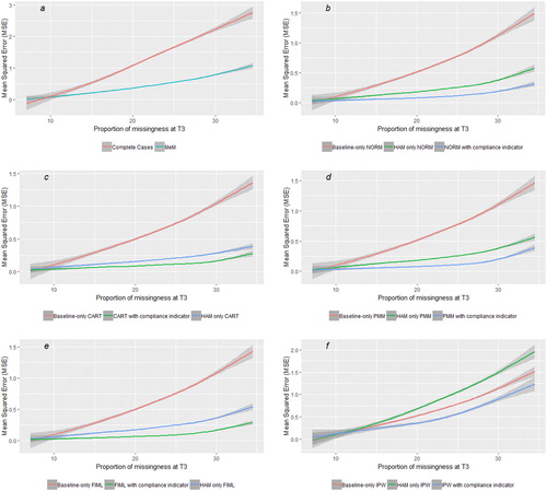
Further visualizations of the performances of different methods depending on trials’ characteristics and of imputed data from the multiple imputation methods are included in the supplementary materials. All methods improve their accuracy with higher proportion of post-discontinuation follow-up (Figures S4(a)–(e)).

4 Discussion

The Estimand framework has established a new foundation for the planning, conduct, and interpretation of clinical trials. Now that a tool that better defines the treatment effect of interest is available, analysis methods need to be aligned with the target of estimation.

We have shown that the use of graphical representation (e.g., in form of m-graph) of the a priori beliefs on the data-generation mechanism allows transparent discussion on the assumption and guides an efficient analysis.

Our main result is that different approaches improve their accuracy including the compliance explicitly represented in a variable. In practice, such variable should be included in the imputation model for imputation-based approaches, as auxiliary variable in likelihood-based methods and as a predictor of missingness in weights-based approaches. For all these methods the inclusion of such variable led to an improvement in accuracy (but not in precision) compared to taking into account post-baseline severity scores only, despite post-baseline severity scores (partially) explaining compliance. The inclusion of this variable allows—under reasonable assumptions—to consider missingness non-informative, even in presence of an informative intercurrent event. The performance of methods that ignore compliance tends toward an overestimation of the treatment effect, in line with the finding from Mehrotra, Liu, and Permutt (2017). The use of a binary variable encoding compliance as part of the imputation model has been recently suggested—limited to noninferiority trials—by Rabe and Bell (2019), whose results are in line with ours. Analogies can also be found with the methods proposed by Carpenter, Roger, and Kenward (2013) and Carpenter et al. (2014) (see also Liu and Pang 2017) and with the placebo multiple imputation proposed by Ayele et al. (2014). However, the methods we endorse are proposed as more directly linked to the data-generating mechanism and as MAR-based main estimators rather than for sensitivity analyses. In addition, the methods we are proposing (depending on the observed distribution of the patients who discontinue treatment but continue follow-up) allows for the initial treatment assignment to still influence post-discontinuation increments.

We have limited our scope to the treatment-policy strategy for handling treatment discontinuation. We acknowledge that estimands that employ other strategies might also be informative—for example, the long-term effect in patients who tolerate treatment or a strategy that handles differentially treatment discontinuation depending on the reason (Callegari et al. 2020). However, this strategy has a special place in a regulatory context (e.g., as mentioned in EMA 2018a, 2018b, 2018c), and in clinical practice as ultimately prescribers will make a decision of treatment assignment, and noncompliance occurs not only in clinical trials but also in practice (Sansone and Sansone 2012).

In line with our expectations, this improvement in accuracy is not recorded when simulations are run in the absence of a treatment effect. However, even in this scenario, the inclusion of this variable does not introduce a bias. Furthermore, it could be argued that this scenario does not necessarily corresponds to all instances of absence of average effect, as it is reasonable to assume that even in absence of an average treatment effect, taking or not taking a treatment could modify the outcome for at least some patients—positively or negatively.

The deterioration of performance of different estimators with a growing proportion of missingness of the outcome highlights the importance of continued follow-up after discontinuation. In practice, this is not always easy to implement as patients might decide to avoid visits in absence of the expectation to benefit from a treatment.

We maintain that our results do not contrast with the recommendation not to include post-baseline measurements in the main analysis (ICH 1998; EMA 2003). However, we suggest that such recommendation should be read as regarding the main analysis model, excluding the imputation model or the propensity score model.

It should be acknowledged that in most cases for data missingness related to treatment discontinuation MNAR is equally reasonable as MAR. Here, we have only used techniques that are suitable for MAR data (and we have simulated MAR data). Further research should investigate sensitivity analyses assuming MNAR.

5 Conclusion

Considering our data and the argument presented above, we can recommend—for the estimation of an estimand that employs a treatment-policy strategy for treatment discontinuation:

• That every effort to continue follow-up of patients who discontinue the treatment is made.

• That assumptions made on data-generating mechanisms, including mechanisms leading to data missingness, are transparently represented, for example, as m-graphs.

• That, consistently with what could be reasonably assumed in most scenarios, observed compliance is represented as a variable and accounted for when working with missing data with any approach.

The European Medicines Agency has had a leading role in the development and adoption of the framework and promotes further research in this field. In particular, more research is needed to develop sensitivity estimators that allow exploring the implications of a wider range of assumptions on the missingness mechanism.

Acknowledgments

We thank Florian Lasch for his comments that significantly improved our article.

Supplementary Materials

See Supplementary Materials for additional figures and details on the simulations.

References

- Ayele, T. B., Lipkovich, I., Molenberghs, G., and Mallinckrodt, C. H. (2014), “A Multiple-Imputation Based Approach to Sensitivity Analysis and Effectiveness Assessment in Longitudinal Clinical Trials,” Journal of Biopharmaceutical Statistics, 24, 211–228. DOI: 10.1080/10543406.2013.859148.
- Baraldi, A. N., and Enders, C. K. (2010), “An Introduction to Modern Missing Data Analyses,” Journal of School Psychology, 48, 5–37. DOI: 10.1016/j.jsp.2009.10.001.
- Breiman, L., Friedman, J. H., Olshen, R. A., and Stone, C. J. (1984), Classification and Regression Trees, Monterey, CA: Wadsworth & Brooks/Cole Advanced Books & Software.
- Callegari, F., Akacha, M., Quarg, P., Pandhi, S., von Raison, F., and Zuber, E. (2020), “Estimands in a Chronic Pain Trial: Challenges and Opportunities,” Statistics in Biopharmaceutical Research, 12, 39–44. DOI: 10.1080/19466315.2019.1629997.
- Carpenter, J. R., Roger, J. H., and Kenward, M. G. (2013), “Analysis of Longitudinal Trials With Protocol Deviation: A Framework for Relevant, Accessible Assumptions, and Inference via Multiple Imputation,” Journal of Biopharmaceutical Statistics, 23, 1352–1371. DOI: 10.1080/10543406.2013.834911.
- Carpenter, J. R., Roger, J. H., and Kenward, M. G. (2014), “Response to Comments by Seaman et al. on ‘Analysis of Longitudinal Trials With Protocol Deviation: A Framework for Relevant, Accessible Assumptions, and Inference via Multiple Imputation’,” Journal of Biopharmaceutical Statistics, 24, 1363–1369.
- Doove, L. L., van Buuren, S., and Dusseldorp, E. (2014), “Recursive Partitioning for Missing Data Imputation in the Presence of Interaction Effects,” Computational Statistics & Data Analysis, 72, 92–104. DOI: 10.1016/j.csda.2013.10.025.
- EMA (2003), “Points to Consider on Adjustment for Baseline Covariates,” available at https://www.ema.europa.eu/en/documents/scientific-guideline/points-consider-adjustment-baseline-covariates_en.pdf.
- EMA (2018a), “Guideline on the Clinical Investigation of Medicines for the Treatment of Alzheimer’s Disease,” available at https://www.ema.europa.eu/en/documents/scientific-guideline/guideline-clinical-investigation-medicines-treatment-alzheimers-disease-revision-2_en.pdf.
- EMA (2018b), “Guideline on Clinical Investigation of Medicinal Products in the Treatment or Prevention of Diabetes Mellitus” (draft), available at https://www.ema.europa.eu/en/documents/scientific-guideline/draft-guideline-clinical-investigation-medicinal-products-treatment-prevention-diabetes-mellitus_en.pdf.
- EMA (2018c), “Guideline on the Development of New Medicinal Products for the Treatment of Crohn’s Disease,” available at https://www.ema.europa.eu/en/documents/scientific-guideline/guideline-development-new-medicinal-products-treatment-crohns-disease-revision-2_en.pdf.
- Enders, C. K. (2008), “A Note of the Use of Missing Auxiliary Variables in Full Information Maximum Likelihood-Based Structural Equation Models,” Structural Equation Modeling: A Multidisciplinary Journal, 15, 434–448. DOI: 10.1080/10705510802154307.
- Finkbeiner, C. (1979), “Estimation for the Multiple Factor Model When Data Are Missing,” Psychometrika, 44, 409–420. DOI: 10.1007/BF02296204.
- Hamilton, M. (1960), “A Rating Scale for Depression,” Journal of Neurology, Neurosurgery and Psychiatry, 23, 56–62. DOI: 10.1136/jnnp.23.1.56.
- ICH (1998), “Statistical Principles for Clinical Trials,” available at https://www.ich.org/fileadmin/Public_Web_Site/ICH_Products/Guidelines/Efficacy/E9/Step4/E9_Guideline.pdf.
- ICH (2019), “Addendum on Estimands and Sensitivity Analysis in Clinical Trials to the Guideline on Statistical Principles for Clinical Trials E9(R1),” available at https://database.ich.org/sites/default/files/E9-R1_Step4_Guideline_2019_1203.pdf.
- Little, R. J. A. (1988), “Missing Data Adjustments in Large Surveys” (with discussion), Journal of Business & Economic Statistics, 6, 287–301. DOI: 10.2307/1391878.
- Liu, G. F., and Pang, L. (2017), “Control-Based Imputation and Delta-Adjustment Stress Test for Missing Data Analysis in Longitudinal Clinical Trials,” Statistics in Biopharmaceutical Research, 9, 186–194. DOI: 10.1080/19466315.2016.1256830.
- Mehrotra, D. V., Liu, F., and Permutt, T. (2017), “Missing Data in Clinical Trials: Control-Based Mean Imputation and Sensitivity Analysis,” Pharmaceutical Statistics, 16, 378–392. DOI: 10.1002/pst.1817.
- Mohan, K., Pearl, J., and Tian, J. (2013), “Graphical Models for Inference With Missing Data,” in Advances in Neural Information Processing Systems, pp. 1277–1285.
- Mohan, K., and Pearl, J. (2019), “Graphical Models for Processing Missing Data,” arXiv no. 1801.03583.
- National Research Council (2010), The Prevention and Treatment of Missing Data in Clinical Trials, Washington, DC: National Academies Press.
- Pearl, J. (1995), “Causal Diagrams for Empirical Research,” Biometrika, 82, 669–688. DOI: 10.1093/biomet/82.4.669.
- Pearl, J., and Paz, A. (1985), “GRAPHOIDS: A Graph-Based Logic for Reasoning About Relevance Relations,” UCLA Computer Science Department Technical Report 850038 (R-53).
- Permutt, T. (2019), “Treatment Effects, Comparisons, and Randomization,” Statistics in Biopharmaceutical Research, 12, 45–53. DOI: 10.1080/19466315.2019.1647874.
- Permutt, T. (2020), “Do Covariates Change the Estimand?,” Statistics in Biopharmaceutical Research, 12, 45–53.
- Potter, F. J. (1993), The Effect of Weight Trimming on Nonlinear Survey Estimates, San Francisco, CA: American Statistical Association.
- R Core Team (2018), R: A Language and Environment for Statistical Computing, Vienna, Austria: R Foundation for Statistical Computing, available at https://www.R-project.org/.
- Rabe, B. A., and Bell, M. A. (2019), “A Conservative Approach for Analysis of Noninferiority Trials With Missing Data and Subject Noncompliance,” Statistics in Biopharmaceutical Research, DOI: 10.1080/19466315.2019.1677493.
- Rosseel, Y. (2012), “lavaan: An R Package for Structural Equation Modeling,” Journal of Statistical Software, 48, 1–36. DOI: 10.18637/jss.v048.i02.
- Rubin, D. B. (1976), “Inference and Missing Data,” Biometrika, 63, 581–592. DOI: 10.1093/biomet/63.3.581.
- Rubin, D. B. (1986). “Statistical Matching Using File Concatenation with Adjusted Weights and Multiple Imputations,” Journal of Business & Economic Statistics, 4, 87–94.
- Rubin, D. B. (1987), Multiple Imputations for Nonresponse in Surveys, New York: Wiley.
- Sansone, R. A., and Sansone, L. A. (2012), “Antidepressant Adherence: Are Patients Taking Their Medications?,” Innovations in Clinical Neuroscience, 9, 41–46.
- Schafer, J. L. (1997), Analysis of Incomplete Multivariate Data, London: Chapman & Hall.
- Schafer, J. L., and Graham, J. W. (2002), “Missing Data: Our View of the State of the Art,” Psychological Methods, 7, 147–177. DOI: 10.1037/1082-989X.7.2.147.
- Seaman, S. R., and White, I. R. (2013), “Review of Inverse Probability Weighting for Dealing With Missing Data,” Statistical Methods in Medical Research, 22, 278–295. DOI: 10.1177/0962280210395740.
- van Buuren, S. (2012), Flexible Imputation of Missing Data, Boca Raton, FL: Chapman & Hall/CRC.
- van Buuren, S. (2018), “R Package: Multivariate Imputation by Chained Equations.”