It’s the Selection’s Fault—Not the p-Values’: A Comment on “The Role of p-Values in Judging the Strength of Evidence and Realistic Replication Expectations”

We would like to congratulate Dr. Eric Gibson on his very scholarly review on the p-value and the controversy surrounding its role in the replicability crisis. It was written from a point of view that appreciates the value of the p-value and embraces its use. We can only join the author in his point of view. To his discussions of the benefits, we would merely like to add that the p-value can be applied under a minimal set of assumptions, and only at the null hypothesis. Moreover, these assumptions can be assured by conducting a well-designed randomized experiment analyzed by a nonparametric method. No other method, frequentist, likelihood-based, or Bayesian, can offer such freedom from modeling assumptions.

We, therefore, focus our comments on the five steps Gibson (2020) proposes for the best practice for the use of p-values. The five steps are (approximately quoted):

1. Illustrate the force of the p-value by the scope of nonnull effects it excludes and the range of meaningful values it supports.

2. Apply the appropriate adjustments for the effects of multiplicity and selective inference.

3. Discount the postulated effect size when planning a follow-up study to account for the effects of publication and selection bias, and low power.

4. Interpret the p-value as a continuous measure on a log scale as -log${}_{10}(p)$.

5. Differentiate between exploratory and confirmatory research.

We have some short comments about (1), (4), and (5). We discuss in some length the other two that address the two forms of selection.

As to the harm caused by ignoring the effect of selection when multiple inferences are evident in the article, we have already argued repeatedly that the reporting of raw p-values without their selection adjusted counterpart, as demonstrated in the PRAISE study, has a devastating effect on the replicability of scientific results (Zeevi et al. 2020). We use this opportunity to demonstrate how to uncover the scale of selection in a complex study such as PRAISE-1, and how it can nevertheless be effectively analyzed using a hierarchical false discovery rate (FDR) approach.

As to the discounting of the effect size needed in view of publication bias and low power, we explain and demonstrate how conditional estimators and confidence intervals can shed light on the estimated effect size, without relying on assumptions about effect size and power.

1 Some Short Comments

Illustrating the force of p-value as suggested in Gibson (2020) Step (1), can also be effectively achieved by the usual construction of a confidence interval from tests of the null hypotheses at the entire range of potential effects. Either way, that means stepping out of the safer domain of the null hypothesis for which the study was designed, so further modeling assumptions are needed. We emphasize that confidence intervals should be built with concern about their being affected by selection, just as argued about the p-values. In the case of the NEJM editorial mentioned by Gibson (2020) this is not the case, and confidence intervals are “excused” for being adjusted for selection, unlike p-values.

The recommendation in Step (4) is not only justifiable but also intuitive: with no reliance on formal justifications, it has become a common practice to plot p-values on a -log₁₀ scale when many are computed. In genomewise association studies, the regularly used Manhattan plot displays the p-values at locations on the genome using a logarithmic scale.

We definitely agree that the distinction between exploratory and confirmatory studies, emphasized in Step (5), is an important one. These two types often exist within a single research effort, which makes it more difficult to distinguish. This distinction should be reflected not only in the level of significance chosen, as suggested, but also in the type of protection taken against the effect of selection. Familywise error-rate control over a very limited family of potential discoveries may be needed in a confirmatory analysis, while FDR control over a broader family may be more appropriate for exploratory analysis. Too often, we read that since the study of the many secondary endpoints is exploratory, we need not address selection at all (the NEJM editorial being a case in point). Still, researchers down the road do select these “significant” ones for further study, whether their significance is judged by p-values or by confidence intervals not covering 0. Ignoring selection in exploratory research is a dangerous practice, as demonstrated in the PRAISE-I relevant example of Packer et al. (1996) discussed by Gibson (2020).

2 Multiplicity and Selection: A Reanalysis of the Effect of Selection in PRAISE-1 Trial

Even when a study is preregistered, the multiple comparisons evident in the reported article can lead to an overestimation of the statistical significance of the outcome. The PRAISE-1 presented by Gibson (2020) is a good example, where amlodipine reducing mortality by 48% in the nonischemic subgroup of patients ($p<0.001$), attracted a failed replication effort. This seems very surprising given the strong statistical significance of the original result. Gibson notes that in view of the primary comparison yielding a negative result, 8 comparisons in total were examined (displayed in Figure 1 under the primary event Morbidity&Mortality and the secondary event Mortality). The $p<0.001$ significance was presented without any correction for being selected out of the 8 inferences conducted, so the effect of selection is at work. The most straightforward correction using Bonferroni to control for the familywise error-rate results in an adjusted p-value < 0.008. Controlling the FDR by the Benjamini–Hochberg procedure (1995, hereafter BH) yields the same value.

Fig. 1 The hypotheses being tested in the PRAISE-I study and their hierarchical structure. Families are visualized by the dashed rectangles.

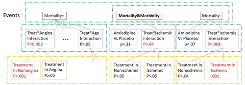
A closer look at the article reveals that the selection is made from a larger pool. While the interaction of the treatment with ischemic status and the resulting subsets are among the 8 Gibson refers to, the interaction of the treatment with seven other criteria are also used to create subgroups. The footnote at the table reports that all interactions were tested (with only one significant), and then the treatment is compared to placebo in each subgroup. Thus, Table 3 in the PRAISE-I study carries 14 more comparisons, reported by unadjusted confidence intervals. Only one of these, in the patients with no Angina history, results in a p = 0.001. A crude count of the inferences performed is the 8 noted by Gibson, plus 7 interactions and 14 comparisons in the subgroups, totaling 29 inferences.

Moreover, an exploratory phase to PRAISE-1 is indicated, when the event of mortality is somewhat modified to include deaths following morbidity events (Mortality + in our notation), a modification noted in a second footnote to the table. It is hard to believe that Mortality and Mortality&Morbidity were not inspected as Mortality + was in the subgroups. It is highly likely that they were not reported as there was no significant result. Thus, it seems that in the exploratory phase of the study, 75 inferences were made. Bonferroni adjustment would have yielded an adjusted p-value of 0.075.

However, not all inferences are made equal. A finding of interaction per se does not lead to a new follow-up study in the same way that the discovery of an effect in a subgroup does, and hence they are not exchangeable in meaning. If only treatment versus placebo comparisons are considered, there are one primary and 16 subgroups (yellow boxes in Figure 1) times the 3 types of events, resulting in 51 inferences. Bonferroni adjustment yields adjusted p = 0.051 for the two most significant ones, but we may just as well be satisfied with control over the FDR. We can use the fact that the inferences are organized into 3 families, each corresponding to one type of event, and use the BH to test this family-of-families.

Family of families testing (Benjamini and Bogomolov 2014)

1. For each of the identified by the type of event, we test the global null hypothesis (no difference in any of the comparisons in the family). For this purpose, calculate the smallest BH adjusted p-value in the family. These are $p_1^{\ast }>0.05$ for the family of the primary event of Morbidity&Mortality, $p_2^{\ast }=0.001*17$ for the family of Mortality and $p_3^{\ast }=0.001*17$ for Mortality+.

2. Test the family-of-families consisting of the above 3 global null hypotheses using BH; since 0.017 <(2/3)0.05, the families of Mortality and Mortality + are rejected.

3. Proceed with each rejected family and test with BH at level (2/3)0.05; the originally two most significant ones will be rejected, one in each rejected family (red script in yellow boxes in Figure 1).

4. Their adjusted p-value is $p^{\mathit{FDR}}=0.001*17*3/2=0.0255$.

The above approach uses the hierarchical family-of-families structure but still ignores the role that interaction testing plays. Instead, we can organize the inferences into a three layers tree, where the interaction of the treatment with a factor leads to the two comparisons in the subgroups generated by the factor. This structure is displayed in Figure 1 and can be tested by TreeBH of Bogomolov et al. (2020), which generalizes the method of Benjamini and Bogomolov to more than two levels. The method was adapted to complex studies involving ANOVA in Zeevi et al. (2020).

In our case, one starts with the lowest families (yellow). The BH adjusted p-values turns out to be above 0.05 for the Morbidity/Mortality family, and 0.001*2 for the two families with a statistically significant comparison. We then go to the next level up using (i) and then again one up using (i) again. Now we have a p-value for the three event type families. Test the family of three types, using BH as before. Wherever rejected, proceed to test the family of interactions and primary comparison as one family, then again wherever rejected, proceed to test the two comparisons within. Because we have a single highly significant p-value in each family of two, and a single significant interaction in the family, the resulting adjusted p-values are as before.

We have demonstrated five points with our analysis of this example. (i) A study can include both a confirmatory stage and an exploratory stage. (ii) The scale of multiplicity from which selection is made and is evident in the published work can be much larger than what meets the eye first; often, some digging is needed to uncover its full scale. (iii) Care is needed in identifying the families of inferences involved and their structural relationships. (iv) Hierarchical FDR controlling methods are natural and can buy power. (v) The failed replication of the treatment with 0.001 significance in PRAISE-I is much less dramatic in view of the treeFDR adjusted p-value of 0.0255. The latter still indicates some potential benefit, being less than the 0.05 threshold for event occurring by chance, but its effect size assessment should rely on the discussion in the next section as well.

3 Discounting the Postulated Effect Size: A Conditional Approach

Gibson’s warning about the need to discount an observed significant effect size hinges on the sample sizes in the study and the true effect, namely on its (unknown) power. His Figure 8 presents simulations result in a low power case and in a case with a higher power (generated by doubling the low power effect size). Gibson demonstrates visually how a significant result exaggerates the effect size, and that a significant result in the wrong direction can be encountered when the power is low.

In the context of the Psychological Reproducibility Project, mentioned in Gibson (2020), the replication target was chosen because it was an important and statistically significant result (at the customary $p ⩽ 0.05$) in 98 of the 100 studies. We have shown that once the statistical analysis is conditioned on the estimator passing the 0.05 threshold, conditional confidence intervals and conditional maximum likelihood estimators (MLEs) offer a more realistic point of view on the effect size (Zeevi et al. 2020). The idea is that the distribution of the effect’s estimator is truncated at the significance threshold Gaussian, rather than full-scale Gaussian. Moving around the hypothesized effect size, the shape of the truncated Gaussian changes, so evaluating the acceptance regions becomes more complicated. Yet, these tests can be inverted to get valid confidence intervals. In particular, we use the Weinstein, Fithian, and Benjamini (2013) construction of such conditional confidence intervals, which further try to balance length and the intrusion into the other side of zero.

To demonstrate the performance of these conditional tools we recreated Figure 8 in Gibson (2020). The blue to yellow dots display 50,000 z scores randomly created as in the original article. The vertical black line represents the significance threshold of one-sided 0.05, which implies a two-sided test at the 0.1 level. All points fall on a single curve in both scenarios. However, their density on the curve changes, as is evident from the two marginal densities displayed, as well as the color on the curve that conveys the density: from high (yellow) to low (blue). Light red dots are 90% conditional CIs of Weinstein, Fithian, and Benjamini (2013) for significantly positives results, while the dark red dots represent these CIs for significantly negative results. The same color scheme in pink is applied to the conditional MLE. The horizontal orange dashed line is the true parameter (Figure 2).

Fig. 2 A recreation of Figure 8 from the original article with the corresponding two panels of higher (right) and lower (left) power. The blue to yellow dots are 50,000 z-scores randomly created as in the original article. The vertical black line represents the significance threshold of one-sided 0.05, which implies a two-sided test at the 0.1 level. Red and purple dots are conditional CI and conditional MLE respectively, where a lighter color represents a positive statistically significant result and a darker color represents a significant result in the wrong direction.

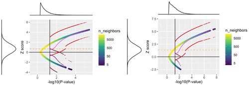
It is evident that as the p-value gets close to the threshold, the conditional CI is widening in the direction of 0, even crossing it to the other side. In particular, when the estimator is negative, even if the effect is statistically significant, the conditional confidence interval does include positive effect sizes in most, failing only in 4.3% ± 0.1%. As the p-value gets far from the threshold, the conditional confidence interval reverts to the unconditional one because the conditional distributions centered further away from the threshold are close to the unconditional ones. The overall coverage of the true effect by the conditional CIs is 90% ± 0.1% as designed.

This performance is the same regardless of the true effect size. The curve and confidence intervals are the same in both power scenarios, and what changes from low power to higher power is just the distribution of points along the curve, as is evident from the two marginal densities (and a few fewer points on the curve in the lower right tail).

Unfortunately, the conditional p-value or conditional confidence intervals cannot serve by themselves as a new criterion. A new criterion will imply a new threshold, and we are back at square one. Similarly, using 0.005 as a threshold, the same “threshold contraction” will occur, resulting in over-optimism about effect size when the significance of a result is 0.004.

In summary, we thank Gibson for writing the article, which expresses nicely many ideas about the p-value that we share. We thank the editor for giving us the opportunity to express this support, and further offer some methodological developments that give the tools for addressing selective inference more effectively without losing rigor, and for showing a more realistic attitude toward the selected.

Additional information

Funding

This work was supported by H2020 European Research Council through Human Brain Project and US–Israel Binational Science Foundation grant 0604317633.

References

- Benjamini, Y., and Bogomolov, M. (2014), “Selective Inference on Multiple Families of Hypotheses,” Journal of the Royal Statistical Society, Series B, 1, 297–318. DOI: 10.1111/rssb.12028.
- Benjamini, Y., and Hochberg, Y. (1995), “A Simple and Powerful Approach to Controlling the False Discovery Rate in Multiple Testing,” Journal of the Royal Statistical Society, Series B, 57, 289–300.
- Bogomolov, M., Peterson, C. B., Benjamini, Y., and Sabatti, C. (2020), “Hypotheses on a Tree: New Error Rates and Testing Strategies,” Biometrika, DOI: 10.1093/biomet/asaa086/.
- Gibson, E. W. (2020), “The Role of p-Values in Judging the Strength of Evidence and Realistic Replication Expectations,” Statistics in Biopharmaceutical Research, DOI: 10.1080/19466315.2020.1724580.
- Packer, M., O’Connor, C. M., Ghali, J. K., Pressler, M. L., Carson, P. E., Belkin, R. N., Miller, A. B., Neuberg, G. W., Frid, D., Wertheimer, J. H., and Cropp, A. B. (1996), “Effect of Amlodipine on Morbidity and Mortality in Severe Chronic Heart Failure,” New England Journal of Medicine, 335, 1107–1114. DOI: 10.1056/NEJM199610103351504.
- Weinstein, A., Fithian, W., and Benjamini, Y. (2013), “Selection Adjusted Confidence Intervals With More Power to Determine the Sign,” Journal of the American Statistical Association, 108, 165–176. DOI: 10.1080/01621459.2012.737740.
- Zeevi, Y., Astashenko, S., Meir, A., and Benjamini, Y. (2020), “Improving the Replicability of Results From a Single Psychological Experiment,” arXiv no. 2006.11585.