Dynamic Monitoring of Ongoing Clinical Trials

Abstract

In late 2019, the U.S. FDA updated a new Guidance for Industry on Adaptive Designs for Clinical Trials of Drugs and Biologics. The guideline encourages developing and implementing innovative trial designs for future clinical trials. Group sequential, sample size re-estimation, and adaptive group sequential procedures have been very useful for improving the efficiency of conducting trials for decades. However, they face some challenges in operational aspects which limited their potentials. In this article, we introduce a procedure that addresses these issues. Our proposed procedure has the capability of providing anytime accessibility of the whole up-to-date data history. The procedure is largely built on the proven adaptive group sequential design theories and combined with advanced eClinical technologies in trial management to elevate the trial design and monitoring to a more dynamic level. The construct of a new trial monitoring screen is illustrated with real trial examples. The advantages of anytime accessibility of data and the monitoring a trial with the whole data history and trend are delineated. Data monitoring committees, sponsors and regulatory authorities are important stakeholders in the discussion of how future clinical trials should be monitored with respect to timing and frequency.

KEYWORDS:

• Adaptive design
• Data and safety monitoring board
• Data Monitoring Committee
• Dynamic data monitoring
• Group sequential design

1 Introduction

In November 2019, the U.S. FDA issued a new draft Guidance for Industry on Adaptive Designs for Clinical Trials of Drugs and Biologics (Center for Drug Evaluation and Research Food and Drug Administration 2019), updating the previously published 2018 and 2010 drafts. This new guidance reflects the agency’s most recent view on developing and implementing innovative trial designs for future clinical trials. Among others, the group sequential design (GSD), sample size re-estimation/re-assessment (SSR), and adaptive group sequential design (AGSD) are referred in the regulatory guidance.

In the classical GSD, interim analyses are conducted at predefined time-points and predetermined number of tests (Pocock 1977; O’Brien and Fleming (OBF) 1979; Tsiatis 1982). The classical GSD was much enhanced by the alpha-spending function approach (Lan and DeMets 1983; Lan and Wittes 1988; Lan and DeMets 1989; Lan, Rosenberger, and Lachin 1993) with flexible analysis schedules and frequencies during the trial. GSD is useful for making early study termination decisions by properly controlling the overall Type I error rate. The study protocol prespecifies a fixed maximum information.

A major consideration in clinical trial design is to estimate adequate amount of information needed to provide the desired study power under a specific alternative. For this task, both GSD and the fixed sample design depend on data from earlier trials to estimate the maximum amount of information needed. The challenge is that such estimates from prior or external source may not be reliable because of perhaps different patient populations, medical procedures, or other trial conditions. Thus, the prefixed maximum information in general, or sample size in specific, may not provide the desired power. Sample size recalculation procedures developed in the early 90s by using the interim data of the current trial itself, aim to secure the study power through possibly increasing the maximum information originally specified in the protocol (Wittes and Brittain 1990; Shih 1992; Gould and Shih 1992; Herson and Wittes 1993). See a commentary on GSD and SSR by Shih (2001).

The two methods, GSD and SSR, later joined together and formed the so-called Adaptive GSD (AGSD). Literature include, to name a few, Bauer and Kohne (1994), Proschan and Hunsberger (1995), Cui, Hung, and Wang (1999), Li et al. (2002), Chen, DeMets, and Lan (2004), Posch et al. (2005), Gao, Ware, and Mehta (2008), Gao, Liu, and Mehta (2013), and Bowden and Mander (2014). See Shih, Li, and Wang (2016) for a recent review and commentary. AGSD has amended GSD with the capability of extending the maximum information prespecified in the protocol using SSR, as well as possibly early termination of the trial.

GSD, SSR, and AGSD have been very useful for improving the efficiency of trials. However, they face some challenges as follows.

First, the timing of SSR is not data-dependent. Conventionally, practitioners frequently suggested half-way through the trial. The mid-trial time, however, may not be ideal. Table 1 illustrates the point with two extreme scenarios.

Table 1 Extreme scenarios with preplanned interim analyses.

	SS based		SS based	50% of
True δ	on true	Assumed δ	on assumed	planned SS	Comment
0.2	526	0.4	133	67	Too early
0.4	133	0.2	526	263	Too late

δ is the treatment effect, 90% design power and assume σ = 1.

Second, many clinical trials employ an independent Data Monitoring Committee (DMC) to review the data at prescheduled time-points. Usually, the “snapshot” of data, not the whole data history with trend is presented to the DMC. It would be much helpful if the whole history of data is conveniently made available at DMC meetings. For example, if Trial A’s data was trending up and Trial B’s data was trending down, and assuming that the “snapshot” of data at interim timepoint for both trials was within the predefined stopping boundaries (e.g., Pocock or OBF), the DMC might recommend “go” for both based on the snapshot without seeing the whole data trend. But if the DMC could see that the data for Trial B was trending down and unlikely to turn up, they might recommend terminating the trial earlier to avoid unethical patient suffering and financial waste. On the other hand, if the DSMB could see that the data trend for Trial A was very “hopeful,” yet not able to cross the upper stopping boundary within the planned maximum information (sample size), the DMC could recommend expanding the trial by SSR to make the trial eventually a success.

Third, the statistical theories for GSD/AGSD assumed Brownian motion model on the data observed, which induces a linear drift for the B-values (Proschan, Lan, and Wittes 2006). In actuality, this assumption might be violated due to some known or unknown reasons such as operational learning curve, changes in the protocol or patients, etc. The conventional monitoring reviews may not be able to discover the nonlinearity nature of the B-values.

In this article, we introduce a procedure that addresses the above issues. Our proposed procedure is largely based on AGSD, combined with advanced eClinical technologies in trial management (to be specified next) to enhance the trial design and monitoring to a more dynamic level.

Important theoretical results will be reviewed in Section 2. On the data management technology front, most clinical trials nowadays are managed by an electronic data capture (EDC) system. Treatment assignment and drug dispensing are managed by an interactive responsive technology (IRT) system. By integrating EDC and IRT together, treatment effect on endpoints of interest (safety or efficacy) can be computed automatically and continuously. This automation enables us to develop a dynamic procedure based on AGSD to monitor on-going trials and to modify the trial course in a much more timely and informative fashion. We shall discuss the aspect of “timely and informative” fashion (i.e., at any time with data trend) in detail with respect to the Type I error rate protection in Section 2. Here we first use a metaphor to illustrate the idea and advantage of this “anytime trend-data dependent” monitoring procedure, which we shall call the dynamic design and monitoring (DDM) procedure.

It is now very common for car drivers to depend on a GPS navigation device to guide them to their destinations. There are basically two kinds of GPS devices: build-in GPS for automobiles (Car GPS) and GPS apps on smart phones (Phone GPS). The Car GPS will not alert the driver about the traffic condition on the way if it is not connected to the internet, whereas the Phone GPS can provide up-to-the-minute traffic information and road condition for the driver to select a route with the fastest arrival time. Essentially, Car GPS uses the preplanned information for navigation, whereas a phone GPS uses instantaneous information. The AGSD works more like a Car GPS. It predefines time points for interim analyses. Without knowing when the treatment effect becomes stable as patients sequentially provide their outcomes, the selection of time points for interim analyses usually is made by intuition or convenience, which could be premature (thus giving an inaccurate trial adjustment) or late (thus missing the opportunity for a timely trial adjustment). In contrast, the proposed DDM procedure is analogous to the Phone GPS that can guide the trial’s direction in a timely fashion with immediate data input from the trial as the trial proceeds. Like the Phone GPS, DDM not only displays the accumulated data and trend, but also provides options for actions.

The rest of the article is organized as follows. In Section 2, we summarize the existing important results of AGSD from the literature. These results support the theoretical basis for DDM to ensure that the overall Type I error rate is preserved. In Section 3, we describe key new results, which cover the main advantage of DDM in using the full history of cumulative data instead of only a snap-shot at the time of a DMC meeting. By visualizing the data monitoring “radar” screen, the usual Brownian motion model assumption are checked by examining the trajectory of the data path in the DDM. Section 4 provides a recent example of using DDM to monitor the first phase III clinical trial in treating severe COVID-19 patients with remdesivir, where urgent and frequent data monitoring was required during the pandemic crisis. In Section 5, we discuss future directions of possible regulatory interactions and practical matters that involve DMC in using the DDM.

2 GSD and AGSD Key Results Review

The proposed DDM procedure is largely based on the well-established GSD and AGSD procedures. Their statistical properties, especially the Type I error rate protection, have already been documented in the literature. We will review and summarize some of the results in light of the frequent and data-dependent monitoring as basic key features of the DDM.

2.1 GSD

Besides the relevant references of GSD we cited in Section 1, Scharfstein, Tsiatis, and Robins (1997) provided a general theorem that unifies many of the results in the previous literature on “classical” GSD (i.e., with fixed maximum information and fixed maximum number of analyses) for all the tests using the class of test statistics that are regular and asymptotically linear (RAL), including the efficient Wald statistic. Based on the general structure in their theorem, they then discussed “maximum information trial” design and monitoring procedure. The part of DDM that uses classical GS design and monitoring agrees with the general structure of theirs—if the trial does not alter monitoring schedule and does not involve possible SSR—that is, not consider extension of the originally designed maximum information. The DDM, however, recommends and implements a maximum information trial with the more flexible Lan–DeMets alpha-spending function approach in the schedule and frequency of interim analyses.

Most users of the Lan–DeMets alpha-spending function for GSD appreciate the flexibility of the scheduling and frequency of interim analyses, but some may have concern on the data-dependent and “anytime” data accessibility aspects of the DDM, especially on the impact of the study power and the Type I error rate protection. We address these concerns and quote some interesting results from the literature in the following.

Although we usually plan the frequency of interim analyses in the study design, but when a trial is on-going, it may require fewer or more interim looks than originally planned. If fewer looks are required, then the study will be overpowered. If more looks are needed, then the study will be underpowered; boundaries will be increased. In practice, the underpowering is minimal (Lan and DeMets 1989; Scharfstein, Tsiatis, and Robins 1997). The properties of frequency and timing of interim looks, including a continuity-like property for looks occurring close to each other and a monotonicity property when additional looks are taken, and how past monitoring affects future boundaries were all given in Proschan (1999) and Proschan and Lan (2012).

We recognize that, although it is an advantage of DDM in providing “anytime” accessibility to the data, the frequency of interim analyses conducted by the DMC are still finite in common practice. The “anytime” accessibility feature of the DDM is helpful for DMC’s instantaneous inquiry at a DMC meeting (in case the updated result is needed) or in an emergency situation (such as the example of remdesivir trial for COVID-19 pandemic in Section 4). In the DDM, we do not promote the conservative “continuous” monitoring boundaries while in actuality only occasional monitoring is performed, following the discussions in Lan, Rosenberger, and Lachin (1993). Although data-driven monitoring affects the Type I error rate, but for reasonable α-spending functions, the worse cases of α-inflation are small. Nevertheless, the Type I error rate is protected even under the continuous monitoring scenario. As asserted in Proschan and Lan (2012) “data-driven monitoring cannot inflate the Type I error rate if a continuous-monitoring boundary is used.” In the DDM, such a continuous-monitoring boundary (i.e., OBF-type boundary) is placed on the “radar” monitoring screen just in case this restriction is needed. See Section 4 for a real example.

2.2 AGSD

The DDM further implements the AGSD, where the maximum information needs to be extended using information available at interim analyses. There are many examples in the literature for mid-course changes of the preplanned adaptive design. A real trial example was provided in Müller and Schäfer (2001), where modification on sample size and schedule of interim analyses were based on data inspections. The DDM uses the data trajectory and automates the process in a timely fashion. The SSR is performed by using the conditional power approach. There are several ways to preserve the Type I error rate at the final analysis, including the weighted Z-test—CHW method (Cui, Hung, and Wang 1999), LSW method (Li et al. 2002; Bowden and Mander 2014), and promising zone approach (Chen, DeMets, and Lan 2004; Mehta and Pocock 2011). These methods are reviewed in Shih, Li, and Wang (2016) and are available in DDM as options. The “radar” monitoring screen of DDM, as demonstrated in Section 4, is based on the conditional power with different zones. Most of the time, a two-stage procedure is adequate, that is, the next analysis is the final test following the SSR. However, multiple/group sequential testing after the SSR is also available, for which Gao, Ware, and Mehta (2008) is used. The re-estimated sample size and the critical value calculations to protect the Type I error rate using these methods are implemented in the DDM. The DDM uses the data trajectory and automates the process in a timely fashion.

Notice that the above discussion focused on the Type I error rate protection for early rejection of the null hypothesis. Futility analyses are also an essential part of the sequential monitoring, which would not affect the Type I error rate, as futility is regarded as nonbinding business decision in the view of regulatory agencies. In the DDM, futility analyses based on the cumulative data are also carried out with the assistance of the “radar” monitoring screen, as discussed in Section 3.2. The optimal timing for futility analyses is based on the framework of Xi, Gallo, and Ohlssen (2017); that is, to maximize the benefit of futility analyses in reducing costs (in terms of sample size) with the trade-off in power loss when considering frequency and timing of futility analysis.

3 New Results

3.1 Visual Diagnostic of Brownian Motion Assumption and Sensitivity Analysis Using Data Trend

As alluded to previously, the key feature of the DDM is the anytime accessibility of the whole history of data during the course of a trial for possible frequent and instant monitoring—thanks to the new data management technology. The general theory and framework are the same between DDM and the existing GSD and AGSD. However, with the DDM, the data trajectory, not just a “snap-shot” is available at each interim analysis to the DMC. The existing GSD and AGSD usually do their analyses on a “snap-shot” of the data, which could be misleading when the data deviate from the assumption of Brownian motion. The DDM can check the assumption of the Brownian motion process with the data trend in display. This is best illustrated by an example as follows.

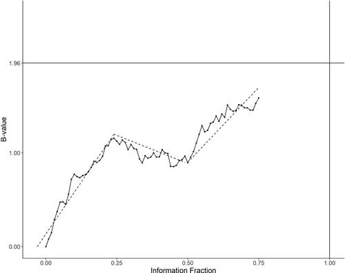
Figure 1 is a data history displayed by B-values B(t), as defined in Lan and Wittes (1988) associated with a RAL test statistic referred in Scharfstein, Tsiatis, and Robins (1997), versus the information fraction t for a study up to an interim analysis at t = 0.75. $B(t)=Z(t)\sqrt{t}$, where Z(t) is the Z-test based on the RAL statistic. Under the model of Brownian motion, we expect to see a linear trend of B(t). In this graph, however, one may suspect that three pieces of linear trend could fit better than just one linear trend. This visual examination is of course not a formal diagnostic test. However, the whole history of data up to the time of an interim analysis obviously helps to suggest performing some sensitivity analysis at t = 0.75.

Fig. 1 Visual display of the trajectory of data.

To be specific, we start with the following well-known result of conditional power given in, for example, Proschan, Lan, and Wittes (2006). Let the final critical value for B(1) be $C_{\alpha }$, which equals 1.96 for α = 0.025 when no multiplicity adjustment is involved. The conditional power at the information time t conditioning on B(t) is given by(1) $$\begin{array}{c}\text{CP}\left(\theta ,t\right)=P\left(B(1)\ge C_{\alpha }|B(t)\right)\\ =1-\Phi \left(\frac{C_{\alpha }-B\left(t\right)-\theta \left(1-t\right)}{\sqrt{1-t}}\right),\end{array}$$(1) where θ is the drift parameter which represents the true (unknown) treatment effect in terms of the B-value. There are many ways of choosing θ in (1). Choice depends on the monitoring objectives, such as the specific value in the alternative hypothesis H_A on which the original sample size and power were based; 0 under H₀; empirical point estimate $\widehat{\theta }=\frac{B(t)}{t}$; some confidence limits based on $\widehat{\theta }$; or some combination of the above, perhaps even with other external information or opinion of a clinical meaningful effect that needs to be detected, etc. Moreover, the predictive power is obtained by averaging $\text{CP}(\theta ,t)$ over a prior distribution of θ. The DDM offers all these options. The most popular choice in the literature is $\widehat{\theta }=\frac{B(t)}{t}$, which is a “snap-shot” of the data at t.

When the graph indicates that a piecewise linear trend rather than one slope fits better for the data path, we may want to perform some sensitivity analysis on the conditional power by considering other choices of θ. For example, in the graph, we see three segments with slope $S_1=\frac{B(t_1)}{t_1}$, $S_2=\frac{B(t_2)-B(t_1)}{(t_2-t_1)}$, $S_3=\frac{B(t_3)-B(t_2)}{(t_3-t_2)}$, respectively, for time period $(0,t_1),(t_1,t_2)$ and $(t_2,t_3)$. A weighted average $w_1{S}_1+w_2{S}_2+w_3{S}_3$ may be used. It is often reasonable to down weigh the earlier trend, judged by the data maturity and/or nature of treatment effect. Notice that $\widehat{\theta }=\frac{B(t)}{t}$ is also a weighted average with the weights proportional to the length of the segment ($w_1=\frac{t_1}{t_3},w_2=\frac{t_2-t_1}{t_3},w_3=\frac{t_3-t_2}{t_3}$) instead of the time order. When performing multiple interim analyses, the weights change and this approach becomes a moving (weighted) average for calculating the conditional power from time to time, with the whole up-to-date data path rather than a “snap-shot” at each time. In DDM, we recommend this approach when the data seem to exhibit nonlinear drift. See Section 4.1 for demonstration by an example.

3.2 “Radar” Monitoring Screen With Four Regions

The DDM uses the conditional power to construct a “radar” screen as its major tool for monitoring an on-going trial. In the literature, while GSD usually divides the action regions to “rejection of H₀ (for overwhelming efficacy),” “acceptance of H₀ (for futility),” and “continuing the trial” in the middle, AGSD further divides the middle into “continuing the trial with or without SSR.” The “continuing with SSR” part is called “promising zone.” In DDM, the rejection region is kept but is on top of a larger region called “favorable,” the promising region is called “hopeful,” and the acceptance region is divided into “unfavorable” and “futility” regions, where the futility region is more restrictive (conservative) than that constructed in the GSD or AGSD. In addition, DDM places a continuous monitoring boundary based on the OBF-type spending function to aid the rejection region as we discussed in Section 2 and in Figure 5 in an example (Section 4.2).

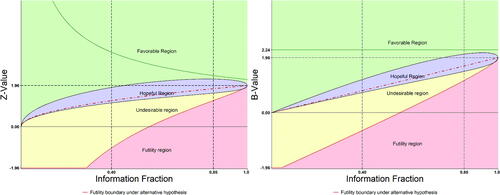
To be more specific, again, this is best illustrated by a graphic example. In Figure 2, the DDM screen with four colored regions based on the B-value (right-hand panel) and Z-value (left-hand panel) are shown in parallel for easy illustration. The Z-value panel is more familiar to general trialists and DMC members including biostatisticians and clinicians, and will be used for application in Section 4, but our discussion in the following will continue with the B-value.

Fig. 2 DDM “radar” monitoring screen with four regions.

3.2.1 The Favorable Region

For simplicity, let us focus on the fixed design for a moment, that is, $C_{\alpha }=Z_{\alpha }$. The discussion can be easily extended to the GSD. When monitoring an on-going trial, we first want to assess whether the conditional power under the current “snap-shot” is greater than $1-\beta$ (say 90%). In other word, whether $B(t)\ge b_1(t,1-\beta )=(Z_{\beta }\sqrt{1-t}+C_{\alpha })t$, derived from Equation (1)(1) $$\begin{array}{c}\text{CP}\left(\theta ,t\right)=P\left(B(1)\ge C_{\alpha }|B(t)\right)\\ =1-\Phi \left(\frac{C_{\alpha }-B\left(t\right)-\theta \left(1-t\right)}{\sqrt{1-t}}\right),\end{array}$$(1) with $\widehat{\theta }=\frac{B(t)}{t}$ plugged in for θ, that is,(2) $$\text{CP}\left(\widehat{\theta },t\right)=1-\Phi \left(\frac{C_{\alpha }-\frac{B\left(t\right)}{t}}{\sqrt{1-t}}\right)=\Phi \left(\frac{\widehat{\theta }-C_{\alpha }}{\sqrt{1-t}}\right).$$(2)

The region $\{B(t)\ge b_1(t,1-\beta )\}$ is considered “favorable” as classified by Mehta and Pocock (2011). $b_1(t,1-\beta )$ is the borderline between the favorable (green color) and the hopeful regions (purple color, to be defined in next section). In this example (Figure 2, $\alpha =0.025$), a selected discrete boundary for rejection region could also be included (depending on the protocol plan) with the OBF-type continuous monitoring boundary (B(t) = 2.24), which is placed on the top for an extreme rejection region.

3.2.2 The Hopeful and Unfavorable Regions

Mathematically, the domain of the Brownian motion $B(t)$ may be beyond 1. Let N₀ be the original sample size per arm to meet an unconditional power requirement, $1-{\beta }^{\prime }$. The adaptive procedure allows changing the sample size at any time, say, at $t=n/N_0$ with observed $B(t)$. Suppose the new per-arm sample size is $N_1>N_0$, which corresponds to the information time $T_1=N_1/N_0$. Let $B(T_1)$ be the potential observation at T₁. To preserve the Type I error rate, the critical boundary $C_{\alpha }=C_0$ must be adjusted to C₁, so that $P(B(T_1)\ge C_1|B(t))=P(B(1)\ge C_{\alpha }|B(t))$ under the null hypothesis. The independent increment property of Brownian motions gives $\Phi (\frac{B(t)-C_{\alpha }}{\sqrt{1-t}})=\Phi (\frac{B(T_1)-C_1\sqrt{T_1}}{\sqrt{T_1-t}})$. Solving for C₁ produces the following formula for the new critical value:(3) $$C_1=\frac{1}{\sqrt{T_1}}\left\{\frac{\sqrt{T_1-t}}{\sqrt{1-t}}\left(C_{\alpha }-B\left(t\right)\right)+B\left(t\right)\right\}.$$(3)

The same idea used for deriving (1) and (2) produces extended conditional power given $B(t)$:$$\begin{array}{c}P\left(B\left(T_1\right)\ge C_1\sqrt{T_1}|B\left(t\right),\widehat{\theta }\right)\\ \hspace{1em}=\Phi \left(\frac{B\left(t\right)+\widehat{\theta }\left(T_1-t\right)-C_1\sqrt{T_1}}{\sqrt{T_1-t}}\right)\\ \hspace{1em}=\Phi \left(\frac{\widehat{\theta }{T}_1-C_1\sqrt{T_1}}{\sqrt{T_1-t}}\right).\end{array}$$

Setting it to be $1-\beta$ and plugging in C₁ from Equation (3)(3) $$C_1=\frac{1}{\sqrt{T_1}}\left\{\frac{\sqrt{T_1-t}}{\sqrt{1-t}}\left(C_{\alpha }-B\left(t\right)\right)+B\left(t\right)\right\}.$$(3) , we get(4) $$T_1-t=\frac{{(Z_{\beta }\sqrt{1-t}+C_{\alpha }-B\left(t\right))}^2}{{\widehat{\theta }}^2\left(1-t\right)}.$$(4)

$T_1=N_1/N_0$ is the new sample size ratio to meet the conditional power $1-\beta$ (generally, we may set $1-\beta =1-{\beta }^{\prime }$).

While designing a trial, we may want to control the sample size ratio not to exceed a maximum affordable budget. Let $R_{\text{max}}$ be the maximum sample size ratio to be considered. From Equation (4)(4) $$T_1-t=\frac{{(Z_{\beta }\sqrt{1-t}+C_{\alpha }-B\left(t\right))}^2}{{\widehat{\theta }}^2\left(1-t\right)}.$$(4) , the sample size ratio R for a given desired conditional power is expressed by$$\begin{array}{c}R=T_1=\frac{N_1}{N_0}=t+\frac{{(Z_{\beta }\sqrt{1-t}+C_{\alpha }-\widehat{\theta }t)}^2}{{\widehat{\theta }}^2\left(1-t\right)}\\ =t+\frac{{(Z_{\beta }\sqrt{1-t}+C_{\alpha }-B\left(t\right))}^2}{{\left(B(t)/t\right)}^2\left(1-t\right)}.\end{array}$$

Solving for $B(t)$ in terms of a given $R_{\text{max}}$ leads to following inequality,(5) $$\begin{array}{c}\frac{\left(Z_{\beta }\sqrt{1-t}+C_{\alpha }\right)t}{t+\sqrt{\left(R_{\text{max}}-t\right)\left(1-t\right)}}\le B\left(t\right)=\frac{\left(Z_{\beta }\sqrt{1-t}+C_{\alpha }\right)t}{t+\sqrt{\left(R-t\right)\left(1-t\right)}}\\ \le \left(Z_{\beta }\sqrt{1-t}+C_{\alpha }\right)\\ \hspace{1em}\times t=b_1\left(t,1-\beta \right).\end{array}$$(5)

Denote $b_2(t,R_{\text{max}})=\frac{\left(Z_{\beta }\sqrt{1-t}+C_{\alpha }\right)t}{t+\sqrt{(R_{\text{max}}-t)(1-t)}}$. The inequality (5) leads to the “hopeful” region for a given $R_{\text{max}}$ in terms of B-value: $b_2(t,R_{\text{max}})\le B(t)\le b_1(t,1-\beta ).$ In the “hopeful” region, the maximum sample size ratio is set to be no more than $R_{\text{max}}$. Note that the conditional power under the current “snap-shot” is $\text{CP}=\Phi (\frac{B(t)/t-C_{\alpha }}{\sqrt{1-t}})$. By replacing $B(t)/t$ with $\frac{\left(Z_{\beta }\sqrt{1-t}+C_{\alpha }\right)}{t+\sqrt{(R_{\text{max}}-t)(1-t)}}$, we map the conditional power in the “hopeful” region so that(6) $$\begin{array}{c}\gamma \left(t,R_{\text{max}}\right)=\Phi \left(\frac{z_{\beta }+C_{\alpha }\left(\sqrt{1-t}-\sqrt{R_{\text{max}}-t}\right)}{t+\sqrt{\left(R_{\text{max}}-t\right)\left(1-t\right)}}\right)\\ \le \text{CP}\le 1-\beta .\end{array}$$(6)

This gives another expression of the “hopeful” region in terms of conditional power. Notice that this $R_{\text{max}}$-defined lower-bound is a decreasing function of t, from $\gamma (0,R_{\text{max}})=\Phi (\frac{z_{\beta }+C_{\alpha }\left(1-\sqrt{R_{\text{max}}}\right)}{\sqrt{R_{\text{max}}}})$ to $\gamma (1,R_{\text{max}})=\Phi (z_{\beta }-C_{\alpha }\sqrt{R_{\text{max}}-1}$). Note that $\gamma (1,R_{\text{max}})$ is the worst case scenario in CP when B(t) falls in the “hopeful” region. When monitoring an on-going trial, we may want to choose a time when CP is not too low (such as <20%) for SSR. Thus, $\gamma (t,R_{\text{max}})$ can be used to select an interim analysis time or a time interval for considering sample size recalculation.

Figure 3 illustrates “favorable” and “hopeful” regions (left panel), and the lower bounds of conditional power while B(t) falls in the “hopeful” region (right panel), with the target conditional power of $1-\beta$ = 0.90 and $R_{\text{max}}=1.5,2.0,3.0$, and 4.0. On the left panel, the “favorable” region is above the line in black and the “hopeful” regions are between lines in black and in other colors corresponding to different $R_{\text{max}}$. As shown, the larger the $R_{\text{max}}$ is, the lower the borderline of “hopeful” region will be or the larger the “hopeful” region will be. The right panel displays the lower bounds of the conditional power which also form the corresponding “hopeful” regions in terms of CP. For example, when $R_{\text{max}}=2.0$, the lower bound of CP ranges from 0.630 (t = 0) to 0.248 (t = 1).

Fig. 3 Favorable and hopeful regions and lower bound of conditional power.

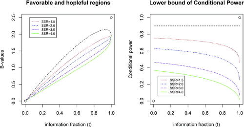
The yellow color region $B(t)<b_2(R_{\text{max}},t)$ in Figure 2 is called “undesirable” region for a moment (only for the sake of being below the “hopeful” region). As the CP on the borderline ranges from 0.630 (t = 0) to 0.248 (t = 1), it is easy to see that even in the “undesirable” region, we may not want to terminate the trial too early. We need to further define a “futile” region to consider possible early termination. The “undesirable” region will be remarked in Section 3.2.4 when we make a summary.

3.2.3 The Futile Region and Monitoring Futility

Futility is also often monitored during a trial, performed either alone or sometimes imbedded with efficacy interim analyses. In either setting, since the decision of whether a trial is futile leading to a decision to stop the trial or not is nonbinding, a futility analysis plan should not be used to modify the Type I error rate control. Rather, futility interim analyses increase the Type II error rate, thus induce power loss of the study. What needs to be considered with futility analyses is the power issue. Frequent futility analyses may induce excessive power loss.

How much power loss would be incurred when a trial is continuously monitored for futility? If futility is monitored by a conditional power (stochastic curtailment) approach, the answer is provided in Lan, Simon, and Halperin (1982) as follows. Instead of conditioning on the current estimate $\widehat{\theta }$, we use ${\theta }^{\ast }$= $Z_{\alpha }+Z_{{\beta }^{\prime }}$ under H_a. When the conditional power (based on ${\theta }^{\ast }$) is lower than a threshold (γ_f), then the trial is deemed futile and may be stopped for futility. Hence, we construct a continuous futility region in terms of B-value: $B(t)\le b_f(t)={\Phi }^{-1}({\gamma }_f)\sqrt{1-t}-(Z_{\alpha }+Z_{{\beta }^{\prime }})(1-t)+Z_{\alpha }.$ See the pink color region in Figure 2. Compared to the original power $1-\beta \prime$, the power loss would be at most $\beta \prime \left(\frac{1}{1-{\gamma }_f}-1\right).$ For example, if the design power is 0.9 and ${\gamma }_f\le 0.5$, we can expect the loss to be no more than 0.1. An ending (unconditional) power of 0.8 may be considered acceptable. For γ_f = 0.20, the power loss is as low as 0.025. The lower the γ_f is, the lower the power loss. In general, the power loss with the uniform threshold γ_f is negligible.

In practice, occasional futility analyses are performed at prespecified interim times t_i by checking whether $\text{CP}(t_i)<{\gamma }_i,i=1,2,\dots ,k$. Unlike the continuous boundary where the futility rule is uniformly applied for all t, choosing γ_i can be flexible depending on the tolerability of CP that we are willing to take at t_i. For example, we may choose smaller γ_i for earlier timepoints compared to later timepoints to avoid early futility stopping. Considering when to conduct futility analyses, we hope the procedure can spot futile situation as soon as possible to save cost as well human suffering from an ineffective therapy. On the other hand, early futility analysis more likely induces power loss for an effective therapy. Thus, we can frame the timing issue of futility analyses as an optimization problem by seeking minimization of the sample size (cost) as the objective while controlling the power loss. This approach which Xi, Gallo, and Ohlssen (2017) developed is implemented in DDM.

3.2.4 Remark

Note that the “undesirable” region is in the sense that it is neither hopeful nor futile. In other word, in this region, owing to the fact that $R>R_{\text{max}}$, sample size increase is infeasible, but the study could not be deemed futile either ($\text{CP}>{\gamma }_f$ under H_a). The effect is still in the positive direction (Z-or B-value > 0). In this case, we would take no decision/action but continue monitoring.

In summary, Let t_k and d_k be the kth interim analysis time and stopping boundary, respectively, $k=1,2,\dots ,K=\text{final}$. We develop a guidance for monitoring on-going trials in DDM, with the understanding that K is only for planning purpose, not a fixed number.

1. Stop the trial early for benefit if $Z(t_k)\ge d_k$ or $B(t_k)\ge$ $d_k\sqrt{t_k}$.

2. If $B(t_k)$ falls in the “futility” region persistently, we could consider stopping the trial for futility. However, as discussed in Section 3.2.3, the decision of futility is nonbinding.

3. In between (1) and (2) above, consider sample size recalculation or continue monitoring without any change:

4. No change if $\text{CP}(t_k)\ge 1-\beta$ or equivalently $B(t_k)\ge (Z_{\beta }\sqrt{1-t_k}+C_{\alpha })t$, but not exceeds $d_k\sqrt{t_k}$, that is, in the “favorable” region.

5. If $\gamma (t_k,R_{\text{max}})\le \text{CP}(t_k)<1-\beta$ (i.e., $B(t_k)$ falls in the “hopeful” region), the trial should continue. If we observe consecutive m (say, 10) points in this region, then re-estimate the sample size. Choice of $R_{\text{max}}$ depends on sponsor’s affordability. For example, set $R_{\text{max}}=3$ if it is acceptable. When sample size is increased, the future boundary values are recalculated as well.

6. If $B(t_k)$ falls in the “undesirable” region, we would take no decision/action but continue monitoring. If B(t) stays in this region persistently, the trial may be recommended for termination for administrative reason such as exceeding the affordable budget.

4 Applications of DDM

In this section, we provide three examples of applying DDM to real clinical trials. The first example is a case where DDM is prospectively planned and used by the DMC of the trial. The second and third examples are retrospectively constructed to illustrate how DDM could have been used for early decision making for a successful and failed trial, respectively.

4.1 Example 1

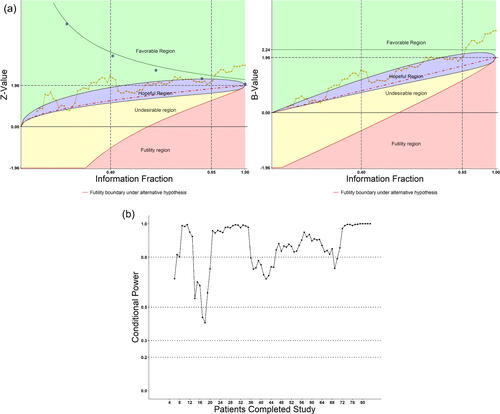
The first double-blind, placebo-controlled clinical trial on the potential antivirus effect of Remdesivir in adult patients with severe COVID-19 was conducted in Wuhan, China (Wang et al. 2020) during January to March 2020. The trial was globally watched during the pandemic crisis and the trial’s DMC was commissioned to make quick and scientifically sound decisions. The DMC faced real challenge to be highly efficient in data transmission and monitoring on key efficacy and safety data, and to function in a very timely manner. The DMC decided to use the eDMC^TM software (CIMS Global) with our DDM “trial-radar” to monitor on-going key safety and efficacy data almost weekly as patients enrolled quickly (Shih, Yao, and Xie 2020). The key efficacy endpoints planned for DMC to monitor was the 6-point ordinal score of the clinical conditions of patients on Days 7, 14, 21, and 28. (However, at early review meetings, DMC also requested instant looks at data for Days 3, 5, and 10, which were considered exploratory.)

According to the plan of DMC’s charter, the treatment groups were compared with respect to their distributions of the ordinal scale using the stratified Wilcoxon–Mann–Whitley (WMW) rank-sum test. As the trial progressed, the trend of the tests was monitored as patients accumulate and treatment days expand. The distribution data were displayed by bar charts and the WMW Rank-sum tests were followed on the DDM “radar” screen. The “radar” screen was constructed with regions of conditional power to show whether the rank-sum test was in “favorable,” “hopeful,” “undesirable,” or “futile” regions, as described in Section 3.2. The trace of the Rank-sum test signals the trend of the trial result from time-to-time as patients being enrolled. During the early stage of the trial, more data cumulated in earlier days and fewer data in later days of follow-up, as expected. Thus, the data examinations were exploratory. Only if a consistent strong signal indicated by the rank-sum test (i.e., falling in the favorable region), would the formal analysis on the protocol-designed primary endpoint, time to clinical improvement (TTCI), be triggered. As time progressed, more patients had longer follow-up data, as expected. Most of times, exploratory analysis was performed, as planned, by examining the “radar” graphs. However, in case it was needed to protect against an inflated false positive rate, especially at the later stage of the trial when sufficient number of patients were enrolled/followed up and we would examine multiple rank-sum tests on Days 7, 14, 21, and 28, the DMC planned to use Hochberg’s step-wise procedure for protecting an overall alpha at 0.025 (1-sided, or 0.05 2-sided) level for this ordinal (secondary) endpoint. Since there was no idea when and how many times the TTCI analysis would be triggered, the group sequential flexible alpha-spending function approach was designed to maintain the overall alpha of 0.025 (1-sided, or 0.05 2-sided) level for the TTCI primary endpoint as well. Moreover, in anticipation of the fast-pace enrollment and relatively short trial duration, and in consideration of the urgent matter for the study, the DMC chose the Pocock-type alpha-spending function for this primary endpoint. Note that the Pocock-type alpha-spending function being concave rather than convex, indicating that more alpha would be spent at earlier than later time, fits the urgent situation of the epidemic; see Shih, Yao, and Xie (2020) for more details. Here, in Figure 4, we demonstrate the path of the Day 28 WMW Rank-sum test Z-values and B-values on the DDM “radar” screen near the fifth DMC meeting around the end of March 2020 when 212 patients (out of 453 planned) finished the Day-28 study treatment and evaluation. The hopeful region (purple color) was set have conditional power satisfying Equation (6)(6) $$\begin{array}{c}\gamma \left(t,R_{\text{max}}\right)=\Phi \left(\frac{z_{\beta }+C_{\alpha }\left(\sqrt{1-t}-\sqrt{R_{\text{max}}-t}\right)}{t+\sqrt{\left(R_{\text{max}}-t\right)\left(1-t\right)}}\right)\\ \le \text{CP}\le 1-\beta .\end{array}$$(6) with $R_{\text{max}}=3$, and $1-\beta =0.90$. The dotted boundary line (red color) inside represents CP = 50%.

Fig. 4 (a) Monitoring treatment effect on Day 28 as patients accumulated on DDM screen. (b) Conditional power on Day 28 as patients accumulated on DDM screen.

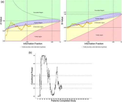
As shown, at early DMC meetings when less than 100 patients (t = 0.22) had their Day-28 evaluations, data fluctuated across favorable and hopeful regions, but the conditional power was greater than 50% most of the times after about 40 patients (t = 0.088). The DMC was optimistic and recommended continuation of the trial. Later, however, the conditional power fell lower than 50% most of the times, and lingered in the unhopeful region when more patients completed their Day-28 evaluations. At the 4th DMC meeting when the Day-28 data from about 180 patients were evaluated, CP was approximately 33%, thus an increase of the sample size was considered. However, the sponsor informed the DMC that the pandemic was already brought under control in China and the study could not continue even with the original sample size, let alone an increase. The study bailed out due to incomplete enrollment on April 2, 2020. Nevertheless, the usefulness of the DDM was well demonstrated in this trial.

A weighted average trend was also performed using 4-piecewise linear drift in the B-value plot using the following four segments when 40, 140, 170, and 212 patients completed, that is, at $t_1=0.088,t_2=0.309,t_3=0.375$, and $t_4=0.468$, respectively. In the B-value plot, the slopes were $S_1=\frac{B(0.088)}{0.088}$ = $\frac{0.3365}{0.088}$ = 3.82, $S_2=\frac{B(0.309)-B(0.088)}{0.309-0.088}=\frac{0.1269-0.3365}{0.309-0.088}=-0.95$, $S_3=\frac{B(0.375)-B(0.309)}{0.375-0.309}=\frac{0.9069-0.1269}{0.375-0.309}=11.82$, and $S_4=\frac{B(0.468)-B(0.375)}{0.468-0.375}=\frac{0.6266-0.9069}{0.468-0.375}=-3.01$, respectively, for these four segments. We choose to down weigh the trend at earlier times, by using $w_1=0.05,w_2=0.30,w_3=0.30,w_4=0.35$ for a sensitivity analysis in addition to the Brownian motion model’s weights (40/220 = 0.18, 100/220 = 0.45, 30/220 = 0.14, 50/220 = 0.23). The resulting weighted average slope was $w_1{S}_1+w_2{S}_2+w_3{S}_3+w_4{S}_4=2.40$.

With 2.40 as the estimate of θ in Equation (1)(1) $$\begin{array}{c}\text{CP}\left(\theta ,t\right)=P\left(B(1)\ge C_{\alpha }|B(t)\right)\\ =1-\Phi \left(\frac{C_{\alpha }-B\left(t\right)-\theta \left(1-t\right)}{\sqrt{1-t}}\right),\end{array}$$(1) , the conditional power $\text{CP}(\theta ,t)$ = 0.469, compared to the snapshot estimate $\widehat{\theta }=0.6266/0.468=1.34$ and $\text{CP}(\widehat{\theta },t)=0.198$. This sensitivity analysis would put the CP in the hopeful region based on the path of the data with subjective weighs. A suggestion for increasing of sample size would be made (and not be accepted by the sponsor due to the same reason of lack of patients since the pandemic was already under control in this case).

4.2 Example 2

This was a multi-center, double-blind, placebo-controlled study with two weeks of daily oral administration of an experimental drug or placebo in subjects with nocturia. The primary endpoint of the study was the 14-day average number of nocturnal voids. The original design was a fixed size design with 80% power at one-side alpha = 0.025. Total of 83 subjects were randomized into the study. At the final analysis, the group with the experimental drug was shown significantly superior to the placebo group (Z-test compared to 1.96).

We have reconstructed the study retrospectively to demonstrate what happened if patients were sequentially monitored with the DDM system according to their time of completing the 14 days of treatment. Figure 5 displays the DDM radar screen plots and the conditional power. As seen, whether with the “continuous” or discrete OB-F boundary (equally spaced, five open blue circles), the test did not cross the corresponding boundaries until t > 0.85. The potential success of the study can be shown from the conditional power plot: the CP was above 80% most of the times starting t > 0.55, after 46 subjects completed the study. This example also demonstrated (1) fluctuations occur in early part of a trial; (2) SSR should not be considered too early when data are still uncertain; (3) CP > 80% during near half of the study, continuing monitoring the trial is helpful; SSR is most likely not needed.

Fig. 5 (a) Retrospectively apply DDM to a real positive clinical trial. (b) Conditional power for the real positive clinical trial.

4.3 Example 3

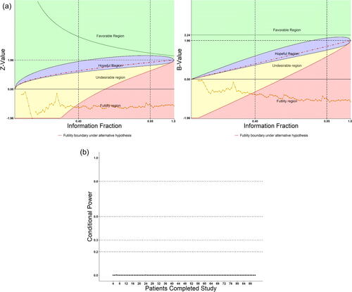
This randomized, double-blind, placebo-controlled study assessed the safety and efficacy of an orally administered experimental drug in patients with nonalcoholic fatty liver disease (NAFLD). The primary endpoint was the change in serum ALT (alanine transaminase) from baseline to 6 months. 91 subjects were randomized to 3 active (dose) groups and placebo. The original design was a fixed size design with 80% power at a one-side alpha = 0.025. At the final analysis, the active groups were shown to be significantly inferior to the placebo group.

Again, we reconstructed the study retrospectively to demonstrate what happened if patients were sequentially monitored with the DDM system according to their time of completing the 6 months of treatment. Figure 6 displays the DDM screen plots of combined active groups versus placebo and the conditional power. As seen, the Z-values were below zero and the conditional powers were nearly zero from the beginning of the study until end. The DDM plots showed the trial entered from the unhopeful region to the futile zone after t = 0.40. The study could have been early terminated for futility if DDM had been used. One might argue that DDM is hardly needed in this extremely negative case. However, since futility is nonbinding, it might also be possible that one time or even more interim analyses with snapshot data would not convince the sponsor to abandon the trial, unless the path of the data showed clearly the hopeless trend, which could be provided by the DDM.

Fig. 6 (a) Retrospectively apply DDM to a real negative clinical trial. (b) Conditional power for the real negative clinical trial.

5 Discussion

Monitoring an on-going clinical trial is an important task and a common practice, and yet it is a difficult task since informed decisions should be made based on observed data but data change from time to time as patients enrolling into the trial. Fortunately, the data collection, digitization, warehousing, retrieval, and analyses technologies have so much advanced in the so-called “artificial intelligence” (AI) era that an integrated tool is now made available to trialists, named DDM, as we present in the article. The DDM tool is founded on well-established adaptive group sequential procedures combined with modern (and the next generation) data management technologies. Two essential features distinguish DDM from the existing methods of data monitoring: anytime accessibility of data and the whole data summary path up to date. We further discuss these two features in the following.

First, “anytime accessibility” does not necessarily imply “continuous monitoring.” “Continuous monitoring” is in the sense of making decision “at every patient.” This is not practical since DMC cannot meet to review data as each patient’s data is available. Currently, the DMC meetings are scheduled periodically but may also change when needed. “Anytime accessibility” is advantageous in the sense that, whenever a need arises, such as from relevant external information or emergency situations, the cumulative data is always available and up to date for analyses. We gave an example of the first Phase 3 treatment trial of remdesivir during the COVID-19 pandemic crisis in this article. It is conceivable that in the future, we will be facing more new diseases or disorders with unfamiliar etiology and trials will be conducted with uncertain mechanism of action toward the target. There will be more situations that trial designs have to be more adaptive and data monitoring will have to be more dynamic in terms of timing and frequency. We do not promote “continuous monitoring” but make data accessibility anytime available with DDM. Just in case an extremely conservative protection of the Type I error risk is demanded, the literature has already proven that the protection of such risk can be achieved, and the continuous monitoring boundary is implemented in the DDM.

Second, the anytime accessibility also means the whole data history is available up to date and the DDM displays the path so that some kind of trend analysis may be evaluated rather than relying on a snap-shot of data at a DMC review meeting. We appreciate that data fluctuate from time to time. That is why some researcher advocated not to perform interim analyses. However, the fact is that almost all clinical trials do conduct interim analyses. Examination of the data trend is clearly more informative than just a snapshot. If data trajectory might be noisy, then the possibility of a snapshot being noisy is even greater. We demonstrate this point with Examples 2 and 3 in this article. We acknowledge that clinical trials all have a time-lag for data to be mature enough for examination. To deal with this phenomenon, a weighted moving average approach is also proposed in this article. This weighted moving average of trends serves as a useful tool for checking the Brownian motion model assumption underlying the usual adaptive group sequential methods.

For operational matters, whether a trial’s DMC is the ideal body to use the DDM tool is subject to debate. Our view is that, DMC should be fully informed and have the capability to access all the data needed to make intelligent recommendations to the trial’s sponsor. DMC is often supported by an independent statistician from the clinical research organization (CRO) contracted by, but independent from, the trial’s sponsor. The DDM could reside at the independent statistician who should have proper training on performing the DDM. The necessary design parameters including those defining the DDM’s radar screen should be fully agreed and thoroughly documented in the DMC Charter.

The world of clinical trials need innovation, and regulatory authorities always encourage innovative trial designs and conduct, as we have seen in the new FDA’s guidance for the pharmaceutical industry. Their understanding and inputs are always needed before buy-in any new methodology to be used for registration trials.

Acknowledgments

We thank the referees and associate editor for their constructive comments. We also would like to thank Dr. Janet Wittes for her critical review of an earlier version of the article.

References

- Bauer, P., and Kohne, K. (1994), “Evaluation of Experiments With Adaptive Interim Analyses,” Biometrics, 50, 1029–1041. DOI: 10.2307/2533441.
- Bowden, J., and Mander, A. (2014), “A Review and Re-Interpretation of a Group-Sequential Approach to Sample Size Re-Estimation in Two-Stage Trials,” Pharmaceutical Statistics, 13, 163–172. DOI: 10.1002/pst.1613.
- Center for Drug Evaluation and Research Food and Drug Administration (2019), “Adaptive Designs for Clinical Trials of Drugs and Biologics Guidance for Industry.”
- Chen, Y. H., DeMets, D. L., and Lan, K. K. G. (2004), “Increasing the Sample Size When the Unblinded Interim Result Is Promising,” Statistics in Medicine, 23, 1023–1038. DOI: 10.1002/sim.1688.
- Cui, L., Hung, H. M., and Wang, S. J. (1999), “Modification of Sample Size in Group Sequential Clinical Trials,” Biometrics, 55, 853–857. DOI: 10.1111/j.0006-341x.1999.00853.x.
- Gao, P., Liu, L. Y., and Mehta, C. (2013), “Exact Inference for Adaptive Group Sequential Designs,” Statistics in Medicine, 32, 3991–4005. DOI: 10.1002/sim.5847.
- Gao, P., Ware, J. H., and Mehta, C. (2008), “Sample Size Re-Estimation for Adaptive Sequential Designs,” Journal of Biopharmaceutical Statistics, 18, 1184–1196. DOI: 10.1080/10543400802369053.
- Gould, A. L., and Shih, W. J. (1992), “Sample Size Re-Estimation Without Unblinding for Normally Distributed Outcomes With Unknown Variance,” Communications in Statistics—Theory and Methods, 21, 2833–2853. DOI: 10.1080/03610929208830947.
- Herson, J., and Wittes, J. (1993), “The Use of Interim Analysis for Sample Size Adjustment,” Drug Information Journal, 27, 753–760. DOI: 10.1177/009286159302700317.
- Lan, K. K. G., and DeMets, D. L. (1983), “Discrete Sequential Boundaries for Clinical Trials,” Biometrika, 70, 659–663. DOI: 10.2307/2336502.
- Lan, K. K. G., and DeMets, D. L. (1989), “Changing Frequency of Interim Analysis in Sequential Monitoring,” Biometrics, 45, 1017–1020.
- Lan, K. K. G., Rosenberger, W. F., and Lachin, J. M. (1993), “Use of Spending Functions for Occasional or Continuous Monitoring of Data in Clinical Trials,” Statistics in Medicine, 12, 2219–2231. DOI: 10.1002/sim.4780122307.
- Lan, K. K. G., Simon, R., and Halperin, M. (1982), “Stochastically Curtailed Tests in Long-Term Clinical Trials,” Communications in Statistics, Part C: Sequential Analysis, 1, 207–219.
- Lan, K. K. G., and Wittes, J. (1988), “The B-Value: A Tool for Monitoring Data,” Biometrics, 44, 579–585. DOI: 10.2307/2531870.
- Li, G., Shih, W. J., Xie, T., and Lu, J. (2002), “A Sample Size Adjustment Procedure for Clinical Trials Based on Conditional Power,” Biostatistics, 3, 277–287. DOI: 10.1093/biostatistics/3.2.277.
- Mehta, C. R., and Pocock, S. J. (2011), “Adaptive Increase in Sample Size When Interim Results Are Promising: A Practical Guide With Examples,” Statistics in Medicine, 30, 3267–3284. DOI: 10.1002/sim.4102.
- Müller, H. H., and Schäfer, H. (2001), “Adaptive Group Sequential Designs for Clinical Trials: Combining the Advantages of Adaptive and of Classical Group Sequential Approaches,” Biometrics, 57, 886–891. DOI: 10.1111/j.0006-341x.2001.00886.x.
- O’Brien, P. C., and Fleming, T. R. (1979), “A Multiple Testing Procedure for Clinical Trials,” Biometrics, 35, 549–556. DOI: 10.2307/2530245.
- Pocock, S. J. (1977), “Group Sequential Methods in the Design and Analysis of Clinical Trials,” Biometrika, 64, 191–199. DOI: 10.1093/biomet/64.2.191.
- Posch, M., Koenig, F., Branson, M., Brannath, W., Dunger-Baldauf, C., and Bauer, P. (2005), “Testing and Estimation in Flexible Group Sequential Designs With Adaptive Treatment Selection,” Statistics in Medicine, 24, 3697–3714. DOI: 10.1002/sim.2389.
- Proschan, M. A. (1999), “A Multiple Comparison Procedure for Three- and Four-Armed Controlled Clinical Trials,” Statistics in Medicine, 18: 787–798. DOI: 10.1002/(SICI)1097-0258(19990415)18:7<787::AID-SIM77>3.0.CO;2-M.
- Proschan, M. A., and Hunsberger, S. A. (1995), “Designed Extension of Studies Based on Conditional Power,” Biometrics, 51, 1315–1324. DOI: 10.2307/2533262.
- Proschan, M. A., and Lan, K. K. G. (2012), “Spending Functions and Continuous-Monitoring Boundaries,” Statistics in Medicine, 31, 3024–3030. DOI: 10.1002/sim.5481.
- Proschan, M. A., Lan, K. K. G., and Wittes, J. (2006), Statistical Monitoring of Clinical Trials—A Unified Approach, New York: Springer.
- Scharfstein, D. O., Tsiatis, A. A., and Robins, J. M. (1997), “Semiparametric Efficiency and Its Implication on the Design and Analysis of Group-Sequential Studies,” Journal of the American Statistical Association, 92, 1342–1350. DOI: 10.1080/01621459.1997.10473655.
- Shih, W. J. (1992), “Sample Size Reestimation in Clinical Trials,” in Biopharmaceutical Sequential Statistical Applications, ed. K. Peace, New York: Marcel Dekker, Inc., pp. 285–301.
- Shih, W. J. (2001), “Commentary: Sample Size Re-Estimation—Journey for a Decade,” Statistics in Medicine, 20, 515–518.
- Shih, W. J., Li, G., and Wang, Y. (2016), “Methods for Flexible Sample-Size Design in Clinical Trials: Likelihood, Weighted, Dual Test, and Promising Zone Approaches,” Contemporary Clinical Trials, 47, 40–48. DOI: 10.1016/j.cct.2015.12.007.
- Shih, W. J., Yao, C., and Xie, T. (2020), “Data Monitoring for the Chinese Clinical Trials of Remdesivir in Treating Patients With COVID-19 During the Pandemic Crisis,” Therapeutic Innovation & Regulatory Science, 54:1236–1255, DOI: 10.1007/s43441-020-00159-7.
- Tsiatis, A. (1982), “Repeated Significance Testing for a General Class of Statistics Used in Censored Survival Analysis,” Journal of the American Statistical Association, 77, 855–861. DOI: 10.1080/01621459.1982.10477898.
- Wang, Y., Zhang, D., Du, G., Du, R., Zhao, J., Jin, Y., Fu, S., Gao, L., Cheng, Z., Lu, Q., and Hu, Y. (2020), “Remdesivir in Adults With Severe COVID-19: A Randomised, Double-Blind, Placebo-Controlled, Multicentre Trial,” Lancet, 395, 1569–1578, DOI: 10.1016/S0140-6736(20)31022-9.
- Wittes, J., and Brittain, E. (1990), “The Role of Internal Pilot Studies in Increasing the Efficiency of Clinical Trials,” Statistics in Medicine, 9, 65–72. DOI: 10.1002/sim.4780090113.
- Xi, D., Gallo, P., and Ohlssen, D. (2017), “On the Optimal Timing of Futility Interim Analyses,” Statistics in Biopharmaceutical Research, 9, 293–301. DOI: 10.1080/19466315.2017.1340906.