Simulation-Based Pharmacokinetics Sampling Design for Evaluating Correlates of Prevention Efficacy of Passive HIV Monoclonal Antibody Prophylaxis

Abstract

We address sampling design of population pharmacokinetics (popPK) experiments in the context of two phase 2b efficacy trials that evaluate the efficacy of VRC01 (vs. placebo) in reducing the rate of HIV infection among 4625 participants. Blood samples are collected at up to 22 study visits from all participants for immediate HIV diagnosis as the primary trial outcome, and stored for future outcome-dependent marker measurements. A key secondary objective of the trials is to evaluate correlates of prevention efficacy among a subcohort of VRC01 recipients in terms of whether the current value of VRC01 serum concentration is associated with the instantaneous rate of HIV infection. To accomplish this, concentrations on a daily grid are estimated via nonlinear mixed effects popPK modeling of observed 4-weekly concentrations.

Given the impracticality of measuring concentrations in all stored blood samples, we devised a simulation-based sampling design framework to evaluate the impact of subcohort sample sizes (m) and sampling schemes of time-points on the accuracy and precision of the popPK model parameters. We accounted for specific study schedules and heterogeneity in participants’ characteristics and study adherence patterns. We found that with m = 120, reasonably unbiased and consistent estimates of most fixed and random effect terms could be obtained without complete sampling of all 22 time-points, even under low study adherence (about half of the 4-weekly visits missing per participant). The described simulation framework is not only novel in its application to popPK sampling design for studying correlates of prevention efficacy in a subcohort of the parent trial, but also flexible in accommodating real-life study setup options, and can be generalized to other single- or multiple-dose PK sampling design settings.

Keywords:

• Population PK analysis
• Sample size determination
• Sampling of PK time-points
• Study adherence
• Two-compartment PK model

1 Introduction

Nonlinear mixed effects population pharmacokinetics (popPK) modeling of drug concentrations is widely used in drug development to account for population-level pharmacokinetic patterns and the dispersion of those parameters between individuals across the population (U.S. Food and Drug Administration 1999). In the two antibody mediated prevention (AMP) efficacy trials of VRC01 (Corey et al. 2021; Gilbert et al. 2017), a human IgG1 broadly neutralizing monoclonal antibody (mAb) against HIV (Wu et al. 2010; Pegu et al. 2014; Ko et al. 2014; Ledgerwood et al. 2015; Mayer et al. 2017), popPK modeling is intended to be employed to estimate individual-specific VRC01 concentrations over time as the first step in the correlates of protection (CoP) analysis of the association between the current value of VRC01 concentration and the instantaneous rate of HIV infection. For example, the estimated serum concentration of VRC01 on a daily scale will be evaluated as a time-dependent covariate in a Cox regression model of time to HIV infection to assess the effect of VRC01 concentration on the risk of HIV infection (Gilbert et al. 2019). This knowledge of CoP is desirable to aid HIV vaccine development by setting benchmark biomarker value for the required potency of a vaccine-induced immune response to putatively achieve a high level of protection against HIV infection. Consequently, this will help define study endpoints in Phase 1 and 2 trials that vet candidate HIV vaccines for their potential efficacy (Gilbert et al. 2017).

In the AMP trials, 4625 HIV-uninfected participants at high risk for acquiring HIV infection are randomized in a 1:1:1 ratio to receive 10 infusions every 8 weeks of 10 mg/kg VRC01, 30 mg/kg VRC01 or placebo, and followed for 80 weeks for the study endpoint of HIV infection. A case-control sampling design is planned to be used in the assessment of CoP, where markers such as serum concentrations of VRC01 are measured from a subcohort of VRC01 recipients—including all HIV infected cases and a random sample of uninfected control participants who remain HIV negative until at least the Week 80 study visit. While complete PK information (e.g., concentration at any given time) is desirable in the study of time-dependent correlates, it is infeasible to sample continuously or on an intensive time scale. Therefore, the full trajectory of VRC01 concentrations over time needs to be estimated via popPK modeling of the concentration data collected at selected time-points for the CoP study. As clinical trial simulation has been generally used in the context to learn about drug effectiveness and safety, and to optimize the design of future trials, the described simulation framework is novel in its application to popPK sampling design for studying correlates of prevention efficacy, but also flexible in accommodating real-life study setup options, and can be generalized to other single- or multiple-dose PK sampling design settings.

In this article, we propose sampling designs of such popPK modeling experiments that will provide input data for the evaluation of CoP in the context of a real clinical trial. Drug exposures and/or sampling times herein are subject to individual-to-individual variation as a result of possible missed infusion or mid-infusion study visits or study dropout, as well as the randomness of the actual time of each study visit within the study-specific visit windows around each target visit date (Figure 1 and supplementary material). In addition, the set of possible sampling time-points are prespecified to accomplish the primary objectives of the trial, and hence optimal design methodologies are usually not directly applicable. To this end, we propose a simulation-based framework to evaluate the impact of samples sizes and sampling schemes of time-points on the accuracy and precision of the popPK model parameters and individual-level concentrations, sidestepping the challenge in accounting for participant and study adherence heterogeneity using traditional optimal experiment design theories (Aarons and Ogungbenro 2011). We illustrate our methods using the AMP correlate study as a concrete example.

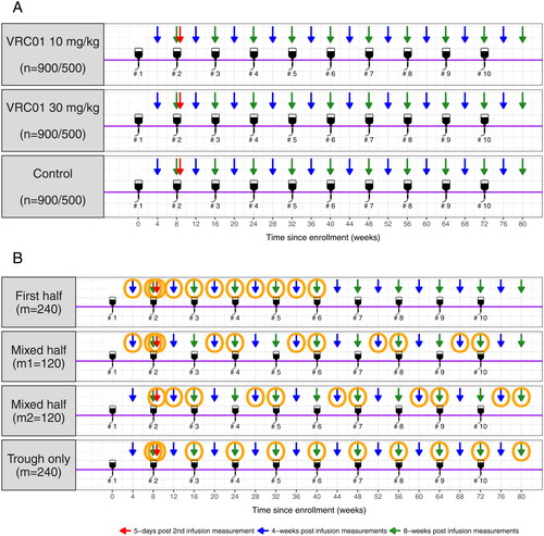
Fig. 1 AMP study schema and marker sampling designs. Panel A: a total of 2700 participants from the Americas and Switzerland trial and 1500 participants from the sub-Saharan Africa trial receive ten IV infusions (#1– #10) of VRC01 at 10 and 30 mg/kg or placebo every 8 weeks at a 1:1:1 randomization ratio. Arrows indicate pre- and post-infusion time-points included in the complete schedule marker sampling design. Panel B: Orange circles indicate sampled time-points in each coarsened schedule marker sampling design. Additional specimen collection times at baseline (week 0) and after week 80 are not included in this figure because data at these time-points mainly contribute to assay control and safety monitoring, not to the PK modeling.

Clinical trial simulation is a common tool to learn about drug effectiveness and safety, and to optimize designs of future trials (Holford, Ma, and Ploeger 2010; Boessen et al. 2011). Not only are our proposed sampling designs novel in their way of meeting both practical concerns and design optimality criteria, our proposed simulation framework is also novel in its application to popPK sampling design for studying correlates of prevention efficacy in a subcohort of the parent study while accounting for real-life study scenarios. The outline of this article is as follows. In Section 2, we introduce the Master popPK model that is used for the simulation of AMP participants’ serum concentration data; the simulation set-up, including different marker sampling designs for the AMP case-control cohort; and the method for estimating popPK model parameters based on the simulated datasets. In Section 3, we compare the performance of different complete and coarsened schedule marker sampling designs in terms of the accuracy and precision of the PK parameter estimates. We draw some conclusions and recommendations in Section 4.

2 Methods

2.1 Master PK Model

A two-compartment model is deemed fitting to describe the PK of VRC01, since this mAb has limited distribution volume, slow clearance, and hence a long half-life (∼15 days). Non-linear mixed effects models are used to describe individual-to-individual processes of drug absorption, distribution, and elimination and how these vary across individuals of different characteristics (e.g., weight, sex, or age). We use the popPK model that best describes the serum concentration data collected in a Phase 1 study of VRC01 (Huang et al. 2017) as the prototype Master model for the simulation of concentration data from AMP participants. Of note, this popPK model is consistent with the one we later constructed based on a subset of HIV-uninfected AMP participants (Huang et al. 2021). In the following, we briefly review the Master popPK model with two levels: the individual-level PK (or structure) model, which describes the intra-individual patterns of serum concentration over time through the processes of drug absorption, distribution, and elimination; and the population-level (or variability) model, which describes the inter-individual variability (IIV) of the processes.

2.1.1 Individual-level PK Model

Let $S(t_{ij})$ denote the VRC01 serum concentration at the jth measurement for subject i. In the Master individual-level PK model, it is defined as$$\begin{array}{c}S(t_{ij})=f(t_{ij},D_i,{\beta }_i)*(1+e{1}_{ij})+e{2}_{ij},\\ \mathrm{\hspace{1em}}\mathrm{\hspace{1em}}\text{for}\mathrm{}i=1,\dots ,m,\mathrm{}j=1,\dots ,m_i,\end{array}$$where f denotes a two-compartment model with dose D_i, ${\beta }_i=({\text{CL}}_i,V_{c_i},V_{p_i},Q_i)$ denotes parameters of f specific to individual i, and the proportional error and additive constant error terms $e{1}_{ij}$ and $e{2}_{ij}$ satisfy, respectively, $\mathrm{E}(e{1}_{ij}|D_i,{\beta }_i)=0,\text{var}(e{1}_{ij}|D_i,{\beta }_i)={\sigma }_1^2$ and $\mathrm{E}(e{2}_{ij}|D_i,{\beta }_i)=0,\text{var}(e{2}_{ij}|D_i,{\beta }_i)={\sigma }_2^2$. There are different ways of parameterizing a compartment model. For their direct physiological significance, CL: clearance rate (L/day), V_c: volume of distribution in the central compartment (L), V_p: volume of distribution in the peripheral compartment (L), and Q: inter-compartmental clearance (L/day) are often a set of parameters used to describe PK processes underlying the observed concentration profiles for a given individual under a two-compartment model.

Specifically, after a single IV infusion, the serum drug concentration at time t (relative to the end of infusion) can be expressed as the sum of two exponential processes—distribution and elimination (i.e., a two-compartment model)$$S(t)=\frac{D}{T_{\text{inf}}}\left[\frac{A}{\alpha }(1-e^{-\alpha T_{\text{inf}}})e^{-\alpha t}+\frac{B}{\beta }(1-e^{-\beta T_{\text{inf}}})e^{-\beta t}\right],$$where $D=$ IV dose amount (mg); $T_{\text{inf}}=$ duration of infusion; α and β are rate constants (slopes) for the distribution phase and elimination phase, respectively ($\alpha >\beta$ by definition); and A and B are intercepts on the y axis for each exponential segment of the curve. Let $k_{12}=Q/V_c$ and $k_{21}=Q/V_p$ represent the first-order rate transfer constants (1/day) for the movement of drug between the central and peripheral compartments. Mathematically, α and β relate to the rate constants k₁₂ and k₂₁ as $\alpha +\beta =k_{12}+k_{21}+k$ and $\alpha \beta =k_{21}k$, where $k=\frac{\text{CL}}{V_c}=\frac{\alpha \beta (A+B)}{A\beta +B\alpha }$ is the rate of drug elimination. In addition, $A=\frac{\alpha -k_{21}}{V_c(\alpha -\beta )}$ and $B=\frac{k_{21}-\beta }{V_c(\alpha -\beta )}$. After multiple doses, serum drug concentration at time t after k doses $D_j\mathrm{}(j=1,.\dots ,k)$ given at time $t_{D_j}(t\ge t_{D_k})$ can then be expressed as written below, based on the superimposed assumption that the PK of the drug after a single dose are not altered after taking multiple doses:$$\begin{array}{c}S(t)=\sum _{j=1}^k\frac{D_j}{T_{{\text{inf}}_j}}[\frac{A}{\alpha }(1-e^{-\alpha T_{{\text{inf}}_j}})e^{-\alpha (t-t_{D_j}-T_{{\text{inf}}_j})}\\ \mathrm{\hspace{1em}}\mathrm{\hspace{1em}}+\frac{B}{\beta }(1-e^{-\beta T_{{\text{inf}}_j}})e^{-\beta (t-t_{D_j}-T_{{\text{inf}}_j})}],\end{array}$$

if $t-t_{D_k}>T_{{\text{inf}}_k}$; or$$\begin{array}{c}S(t)=\sum _{j=1}^{k-1}\frac{D_j}{T_{{\text{inf}}_j}}[\frac{A}{\alpha }(1-e^{-\alpha T_{{\text{inf}}_j}})e^{-\alpha (t-t_{D_j}-T_{{\text{inf}}_j})}\\ \mathrm{\hspace{1em}}\mathrm{\hspace{1em}}+\frac{B}{\beta }(1-e^{-\beta T_{{\text{inf}}_j}})e^{-\beta (t-t_{D_j}-T_{{\text{inf}}_j})}]\\ +\frac{D_j}{T_{{\text{inf}}_k}}\left[\frac{A}{\alpha }(1-e^{-\alpha T_{{\text{inf}}_k}})+\frac{B}{\beta }(1-e^{-\beta T_{in{f}_k}})\right],\\ \mathrm{\hspace{1em}}\mathrm{\hspace{1em}}\text{if}t-t_{D_k}\le T_{in{f}_k}.\end{array}$$

2.1.2 Population PK Model

Let ${\beta }_i=d(a_i,\beta ,b_i),\mathrm{}\text{for}\mathrm{}i=1,\dots ,m$ where d denotes a p-dimensional function, a_i denotes a vector of characteristics for subject i that contributes to explaining IIV, β denotes fixed effects, and b_i denotes random effects. This equation characterizes how elements of β_i vary across individuals due to systematic association with a_i (modeled via β) and unexplained variation in the population represented by b_i. The usual assumptions $\mathrm{E}(b_i|a_i)=\mathrm{E}(b_i)=0$ and $\text{var}(b_i|a_i)=\text{var}(bi)=\Omega$ are implied. In the Master population-level PK model, all four individual-level PK parameters are modeled as log-normally distributed with exponential IIV as follows:$$\begin{array}{c}{\text{CL}}_i={\beta }_{\text{CL}}*\hspace{0.17em}\text{exp}\hspace{0.17em}({\beta }_{\text{BW}.\text{CL}}*({\text{BW}}_i-74.5))*\hspace{0.17em}\text{exp}\hspace{0.17em}(b_{{\text{CL}}_i}),\\ V_{c_i}={\beta }_{V_c}*\hspace{0.17em}\text{exp}\hspace{0.17em}({\beta }_{\text{BW}.V_c}*({\text{BW}}_i-74.5))*\hspace{0.17em}\text{exp}\hspace{0.17em}(b_{V_{c_i}}),\\ Q_i={\beta }_Q*\hspace{0.17em}\text{exp}\hspace{0.17em}(b_{Q_i}),\\ V_{p_i}={\beta }_{V_p}*\hspace{0.17em}\text{exp}\hspace{0.17em}(b_{V_{p_i}}).\end{array}$$

2.2 Marker Sampling Designs

In the parent AMP study, specimens are collected for HIV diagnosis as the primary trial outcome every 4-weekly and at 5 days after the second infusion. Therefore, the marker sampling designs are confined to these available time-points in a subcohort of VRC01 recipients from AMP. We propose two types of marker sampling designs for the evaluation of correlates of prevention efficacy: complete schedule and coarsened schedule (Figure 1). The former design includes concentration data at all time-points of visit attendance from each participant, whereas the latter includes concentration data only at a subset of time-points. Because a total of 61 VRC01 HIV-infected cases are expected at 60% prevention efficacy for both dose groups (i.e., 10 mg/kg VRC01 and 30 mg/kg VRC01) pooled over both AMP trials, for the complete schedule design, we consider sample sizes of m = 30, 60, 120, and 240 HIV uninfected controls. The latter three sample sizes correspond to the numbers of expected controls in the case-control cohort with a 1:1, 1:2, and 1:4 case:control ratio, respectively, whereas m = 30 serves as a reference and represents the 1:1 case:control ratio for a single AMP trial. For the coarsened schedule design, we consider only one sample size of m = 240, but three coarsened schedules that sample roughly half of the complete schedule time-points per participant.

• First half: the first 11 time-points (excluding time 0) out of the total 22 complete schedule time-points are sampled. These time-points include, for every individual, the 4-week and 8-week post-infusion time-points (trough) after the first 5 infusions, in addition to the 5-day time-point after the second infusion.

• Mixed half: time-points after every other infusion are sampled. In addition to the 5-day time-point after the second infusion for every individual, 4-week and 8-week time-points (trough) after the five odd number (1st, 3rd, 5th, 7th, and 9th) infusions are included for one half of the subjects ($m=120)$, and 4-week and 8-week post-infusion time-points after the five even number (2nd, 4th, 6th, 8th, and 10th) infusions are included for the other half of the subjects (m = 120).

• Trough only: trough time-points are sampled. These include, for every individual, the 8-week time-points (trough) after each of the 10 infusions, in addition to the 5-day time-point after the second infusion.

Note that for all 3 coarsened schedules, the 5-day time-point after the second infusion is always included because this time-point is the only one scheduled within a few days of an infusion for the estimation of V_c. These three coarsened schedules are compared to the complete schedule with m = 120, since the same number of 4-week and 8-week post infusion observations are made.

2.3 Simulation Set-up

2.3.1 Study Adherence

Each participant’s infusion and post-infusion visit schedule is simulated according to the AMP protocol specification (Figure 1 and supplementary materials). Briefly, participants receive 10 IV infusions of VRC01 (or placebo). Each infusion visit has a visit window of –7 to +48 days around the scheduled 8-weekly infusion visit target date. Participants’ marker measurements occur at each infusion visit, 4 weeks (visit window: –7 to +7 days) after each infusion, and 5 days (–2 to +2 days) after the second infusion. In the following simulations, for infusion visits, we assume that 80% of the attended visits occur uniformly during the target window of –7 to +7 days and 20% during the allowable window of +7 to +48 days. For post-infusion visits that occur between infusion visits, we assume all attended visits occur uniformly during the specified window.

Overall, we consider four study adherence patterns defined by the combinations of four missing data probabilities: probability of an independently missed single infusion (p₁), probability of an independently missed post-infusion visit (p₂), cumulative probability of permanent infusion discontinuation (r₁), and annual dropout rate (r₂). The four study adherence patterns in terms of (p₁, p₂, r₁, r₂) are: perfect adherence = (0%, 0%, 0%, and 0%), high adherence = (5%, 10%, 10%, and 10%), medium adherence = (10%, 15%, 15%, and 15%), and low adherence = (15%, 20%, 20%, and 20%). At 1 year after trial initiation, the adherence is very high in the ongoing AMP study with rates of (2%, 3%, 5%, and 5%). Nevertheless, a wider range of adherence levels are considered in this article for interpolation purposes and for investigating the robustness of popPK modeling against missing data, relevant if adherence declines in AMP or for future mAb studies.

2.3.2 PK Model Parameter Values

Once participants’ infusion and post-infusion visits are simulated according to the study adherence patterns described above, the Master popPK model described in Section 2.1 is used to simulate VRC01 serum concentration at attended study visits for participants of a given body weight in each VRC01 dose group (10 and 30 mg/kg). The PK parameter values used for the simulation are listed in Table 1, where low covariances between random effects are fixed at zero to increase model stability.

Table 1 Master popPK model parameter values for the simulation of VRC01 time-concentration data.

Term	Parameter	True value	Note
Fixed effects	${\beta }_{\text{CL}}$	0.41	Clearance from the central compartment (CL: L/day)
	${\beta }_{V_c}$	1.92	Central compartment volume (Vc: L)
	βQ	0.87	Inter-compartment clearance (Q: L/day)
	${\beta }_{V_p}$	5.32	Peripheral compartment volume (Vp: L)
	${\beta }_{\text{BW}.\text{CL}}$	0.0072	Body weight influence on CL (/kg)
	${\beta }_{\text{BW}}.V_c$	0.011	Body weight influence on Vc (/kg)
	$\text{var}(b_{\text{CL}})$	0.075	IIV of CL
Variance of	$\text{var}(b_{V_c})$	0	IIV of Vc. Fixed at zero.
random effects	$\text{var}(b_Q)$	0.091	IIV of Q
	$\text{var}(b_{V_p})$	0.14	IIV of Vp
	$\text{cov}(b_{\text{CL}},b_{V_c})$	0	Fixed at zero
	$\text{cov}(b_{\text{CL}},b_Q)$	0.05
Co-variance of	$\text{cov}(b_{\text{CL}},b_{V_p})$	0.062
random effects	$\text{cov}(b_{V_c},b_Q)$	0	Fixed at zero
	$\text{cov}(b_{Vc},b_{V_p})$	0	Fixed at zero
	$\text{cov}(b_Q,b_{V_p})$	0.11
Variance of	${\sigma }_1^2$	0.044	Proportional error
residual errors	${\sigma }_2^2$	0.43	Additive constant error

2.3.3 Computation Software

R version 3.5.1 R Core Team (2016) was used for the simulation of participants’ characteristics and study visit data. The NONMEM software system (Version 7.4, ICON Development Solutions) was used for the simulation and modeling of concentration data. Parallel computing on eight central processing units was employed to speed up computation time via NONMEM.

2.3.4 Simulation Steps

For the complete schedule marker sampling design, we consider a total of 16 scenarios representing combinations of 4 study adherence patterns (perfect, high, medium, and low) and 4 sample sizes (m = 30, 60, 120, and 240). For the coarsened schedule marker design, we consider a total of 12 scenarios representing the combinations of 4 study adherence patterns and 3 coarsened schedules (first half, mixed half, and trough only). The complete schedule datasets with m = 240 are first simulated and the coarsened schedule datasets are extracted from them given the specific design. For each scenario, 1000 datasets are simulated containing participants’ demographic information (body weight and sex), study information (infusion and post-infusion visit time), and serum concentration at attended visits. Depending on the research interest, concentration values on consecutive days or flexible grids can also be simulated to evaluate the modeling/prediction of simulated concentration using sparse data. More details of the specific simulation steps can be found in the supplemental materials.

2.4 Estimation Method and Model Diagnostics

Parameter estimation of the popPK model is based on minimizing the objective function value using maximum likelihood estimation. A marginal likelihood of the observed data is calculated based on both the influence of the fixed effect and the random effect. Different estimation methods for nonlinear mixed effects models have been extensively discussed by other authors (e.g., Plan et al. 2012; Johansson et al. 2014). In this article, due to the sparseness of the simulated data, the Markov chain Monte Carlo stochastic approximation expectation–maximization (SAEM) method (Delyon, Lavielle, and Moulines 1999; Kuhn and Lavielle 2004) is applied to the modeling of the simulated time-concentration data according to the Master PK model. The true values of each PK parameters as specified in Table 1 are used as initial values.

For each simulation scenario, % datasets “converged” is calculated as the proportion of completed runs given the Monte Carlo nature of the SAEM method. For each fixed and random effect, among the B completed runs, relative bias for each run k, ${\text{RBias}}_k$ $=\left(\frac{{\widehat{\beta }}_k-\beta }{\beta }\right)*100$ and relative root-mean-squared error of the estimated PK paramters, RRMSE $=\sqrt{\frac{1}{B}{\sum }_{k=1}^B{(\frac{{\widehat{\beta }}_k-\beta }{\beta })}^2}*100$, as well as the mean squared error of the estimated log-transformed concentration on a daily grid are reported. Of note, the reason for using daily-grid is because the time-point of interest for estimating the concentration could fall on any day after the product administration, and it varies across individuals even within the same study. In addition, reported are coverage probability, CP$=$proportion of datasets with 95% confidence intervals including the true value of the parameter β, as well as the shrinkage estimate for each random-effect term, that is, one minus the ratio of the standard deviation of the individual-level estimate and the estimated variability for the population estimate. As an illustration, a visual predictive check (VPC) is also provided for one randomly selected dataset under the n = 120 high adherence scenario. This scenario is chosen because it closely assimilate the actual AMP studies.

3 Results

3.1 Master popPK Model

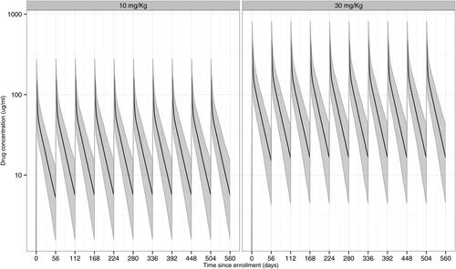
As an illustration, Figure 2 displays two expected population-level time-concentration curves for individuals who are perfectly adherent to the 8-weekly infusion schedule, one for the 10 mg/kg dose and one for the 30 mg/kg dose, based on the master popPK model with $E(b_i)=0,E(e1)=0$, and $E(e2)=0$. The concentrations at each time-point are simulated based on a body weight of 74.5 kg and with the PK parameter values given in Table 1.

Fig. 2 Simulated time-concentration curves under the Master popPK model following ten 8-weekly IV infusions of VRC01 in the 10 mg/kg and 30 mg/kg dose groups with perfect study adherence. Solid lines are the medians; shaded areas are the 2.5% and 97.5% percentiles of the concentrations over 1000 simulated datasets. A body weight of 74.5 kg is used in the simulations.

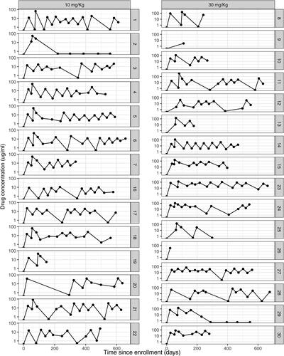
In addition, a random set of the simulated individual-level concentration curves under low study adherence are displayed in Figure 3. For example, individual #2 in the low dose group (left panel) stayed in the study for follow up but discontinued infusions after the first infusion, whereas individuals #9 and #26 in the high dose group (right panel) dropped out of the study right after the first post-infusion visit.

Fig. 3 Simulated time-concentration curves under the Master popPK model following ten 8-weekly IV infusions of VRC01 in the 10 and 30 mg/kg dose groups with low study adherence. With low study adherence, probability of an independently missed single infusion (p₁), probability of an independently missed post-infusion visit (p₂), cumulative probability of permanent infusion discontinuation (r₁), and annual drop out rate (r₂) are assumed to be 15%, 20%, 20%, and 20%, respectively.

3.2 Model Fitting

3.2.1 Complete Schedule Marker Sampling Designs

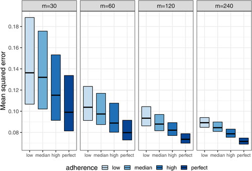
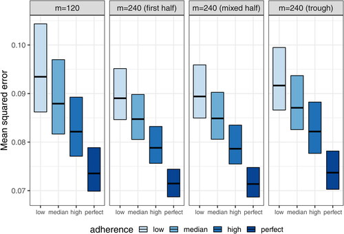
Using the SAEM estimation method, almost all models using datasets under the complete schedule designs converged to obtain final PK parameter estimates for m = 120 and m = 240, whereas a relative low convergence was observed for datasets with m = 30 and m = 60 (Figure 4). This result suggests that a minimal sample size of m = 60 –120 is needed for stable PK model fitting under the described schedule. This pattern is further confirmed when the accuracy and precision of the fixed-effect estimates (Figures 5 and 6; supplementary material, Table 1) and the mean squared error of the estimated concentrations (Figure 7) are examined. Reasonable levels of bias and precision with significant improvements over the small sample sizes are observed for m = 120. On the other hand, m = 240 provides relatively marginal improvements compared to m = 120, except for ${\beta }_{\text{BW}.\text{CL}}$, which characterizes the effect of each individual’s body weight on CL and requires data from a sufficient number of independent subjects for an accurate and precise estimation. For illustration purposes, Figures S1 and S2 (supplementary material) show that reasonably accurate predictions of individual-level daily grid concentrations are achieved and the observed dose-normalized concentration-time data fall largely within the 95% prediction interval in a randomly selected dataset under the m = 120 high adherence scenario.

Fig. 4 Percent of models converged under the complete schedule designs with different levels of study adherence and sample sizes (m = 30, 60, 120, and 240). The four study adherence patterns in terms of (p₁, p₂, r₁, r₂) are: Perfect = (0%, 0%, 0%, and 0%), High = (5%, 10%, 10%, 10%), Medium = (10%, 15%, 15%, and 15%), and Low = (15%, 20%, 20%, and 20%), where p₁ indicates the probability of an independently missed single infusion, p₂ the probability of an independently missed post-infusion visit, r₁ the cumulative probability of permanent infusion discontinuation, and r₂ the annual drop out rate.

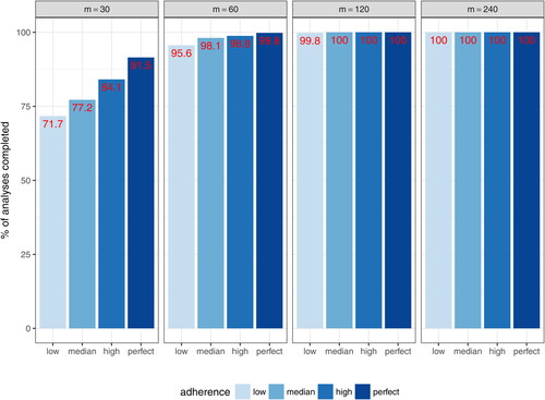
Fig. 5 Relative bias of each fixed-effect PK parameter estimate under complete schedule designs with different sample sizes (m = 30, 60, 120, and 240). ${\beta }_{\text{CL}}$, ${\beta }_{V_c}$, β_Q, and ${\beta }_{V_p}$ indicate the fixed effect for CL, V_c, Q, and V_p, respectively. ${\beta }_{\text{BW}.\text{CL}}$ and ${\beta }_{\text{BW}.V_c}$ indicate the fixed effect of body weight influence on CL and V_c, respectively.

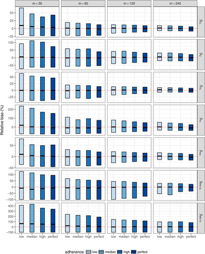
Fig. 6 Relative root-mean-squared errors of each fixed-effect PK parameter estimate under complete schedule designs with different sample sizes (m = 30, 60, 120, and 240). ${\beta }_{\text{CL}}$, ${\beta }_{V_c}$, β_Q, and ${\beta }_{V_p}$ indicate the fixed effect for CL, V_c, Q, and V_p, respectively. ${\beta }_{\text{BW}.\text{CL}}$ and ${\beta }_{\text{BW}.V_c}$ indicate the fixed effect of body weight influence on CL and V_c, respectively.

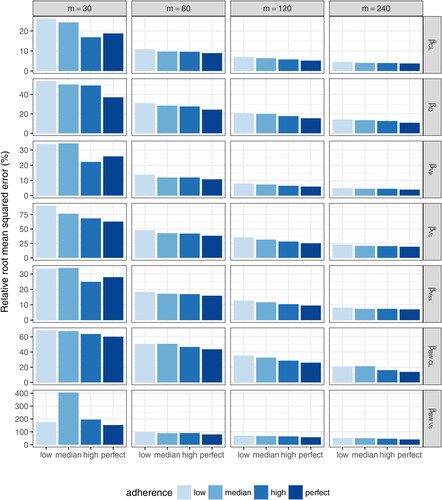
Fig. 7 Mean squared errors of estimated daily grid concentrations under complete schedule designs with different sample sizes (m = 30, 60, 120, and 240).

Due to the unstable estimation for n = 30, we restrict the evaluation of the estimation of random effects to larger sample sizes (Figures S3 and S4, supplementary material). In general, regardless of the sample size, the random effect of the PK parameter Q (inter-compartmental clearance rate) is poorly to the sparsity of data closer to infusion, with only one 5-day post infusion time-point, and the low IIV in Q. On the other hand, the estimation of CL and V_p seems reasonable, with shrinkage generally below 20%–30%. The proportional error term, ${\sigma }_1^2$, is also reasonably estimated with RRMSE $<10\%$ under all scenarios. The estimation of the additive error term, ${\sigma }_2^2$, is relatively poorer, possibly due to the sparsity of data around the assay limit of detection.

3.2.2 Coarsened Schedule Marker Sampling Designs

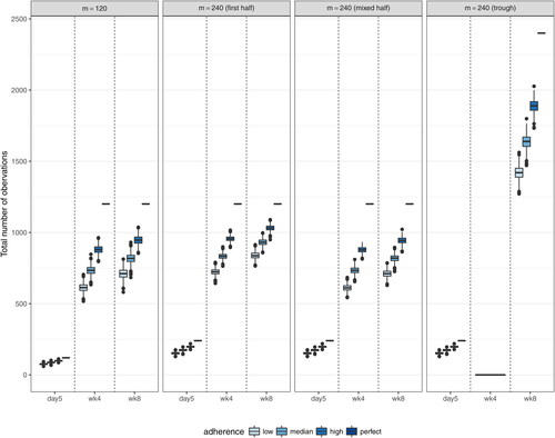
Figure 8 displays the distribution of the total number of observations (5 days after the second infusion, 4 weeks, and 8 weeks after each infusion) based on the 1000 simulated datasets under each of the 12 coarsened schedule scenarios with m = 240, along with the complete schedule design with m = 120. Because about half of the complete schedule time-points are sampled in the coarsened schedules, the total expected number of 4-week and 8-week post infusion observations is the same across the 4 designs. This feature allows a fair comparison across the designs. Meanwhile, the number of 5-day post second infusion observations is doubled in the coarsened schedule designs, because the 5-day post second infusion time-point is the only time-point proximal to an infusion. Hence, this time-point is always sampled from every individual under both the complete and coarsened schedule designs. This consistency allows the assessment of the impact of 5-day post infusion observations on the estimation of various PK parameters.

Fig. 8 Distributions of the total numbers of 5-day post second infusion, 4-week post-infusion, and 8-week post-infusion observations under the complete schedule design with m = 120 and 3 coarsened schedule designs with m = 240. The “First half” design samples the first 11 time-points (excluding time 0) out of the total 22 complete schedule time-points. The “Mixed half” design samples time-points after every other infusion. The “Trough only” design samples only trough time-points. All 3 coarsened schedule designs always include the 5-day post second infusion time-point.

Results showing the accuracy and precision of the fixed-effect estimates and individual estimated concentrations under each coarsened schedule design with m = 240 are displayed in Figures 9–11 and Table 2 (supplemental material). The complete schedule design with m = 120 is included as a reference for comparison purposes. In general, for the estimation of fixed effects, the complete schedule design with half of the sample size provides more accurate but less precise estimates, except that more accurate estimates are obtained for ${\beta }_{V_c}$ and ${\beta }_{\text{BW}.\text{CL}}$ under the “First half” and “Mixed half” coarsened schedule designs. This is likely due to the fact that having more 5-day post infusion observations in the coarsened schedule designs helps improve the estimation of ${\beta }_{V_c}$, which requires data proximal to infusion for an accurate estimation, and having more independent individuals helps improve the estimation of the covariate effect. On the other hand, the accuracy of estimates under the coarsened schedule designs is more impacted by study adherence due to the sparser time-points compared to the complete schedule design. Among the three coarsened schedule designs, the “First half” and “Mixed half” designs have very similar performance and are generally superior to the “Trough only” design, especially for the estimation of ${\beta }_{V_c}$. Similar patterns are observed in the estimation of random effects (Figures S6–S8, supplemental material). Poor estimation of the random effect of inter-compartment clearance (Q) and additive residual error are observed for all designs for the reasons stated above.

Fig. 9 Relative bias of each fixed-effect PK parameter estimate under coarsened schedule designs with m = 240 compared to the complete schedule design with m = 120. ${\beta }_{\text{CL}}$, ${\beta }_{V_c}$, β_Q, and ${\beta }_{V_p}$ indicate the fixed effect for CL, V_c, Q, and V_p, respectively. ${\beta }_{\text{BW}.\text{CL}}$ and ${\beta }_{\text{BW}.V_c}$ indicate the fixed effect of body weight influence on CL and V_c, respectively. The “First half” design samples the first 11 time-points (excluding time 0) out of the total 22 complete schedule time-points. The “Mixed half” design samples time-points after every other infusion. The “Trough only” design samples only trough time-points. All three coarsened schedule designs always include the 5-day post second infusion time-point.

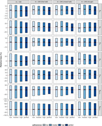
Fig. 10 Relative root-mean-squared errors of each fixed-effect PK parameter estimate under coarsened schedule designs with m = 240 compared to the complete schedule design with m = 120. ${\beta }_{\text{CL}}$, ${\beta }_{V_c}$, β_Q, and ${\beta }_{V_p}$ indicate the fixed effect for CL, V_c, Q, and V_p, respectively. ${\beta }_{\text{BW}.\text{CL}}$ and ${\beta }_{\text{BW}.V_c}$ indicate the fixed effect of body weight influence on CL and V_c, respectively. The ‘First half’ design samples the first 11 time-points (excluding time 0) out of the total 22 complete schedule time-points. The “Mixed half” design samples time-points after every other infusion. The “Trough only” design samples only trough time-points. All 3 coarsened schedule designs always include the 5-day post second infusion time-point.

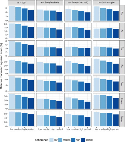
Fig. 11 Mean squared errors of estimated daily grid concentrations under coarsened schedule designs with m = 240 compared to the complete schedule design with m = 120.

4 Conclusions

Nonlinear mixed effects PopPK analysis is known to be suitable for datasets consisting of a few data points per individual from many individuals, in order to estimate popPK parameters accounting for variabilities among individuals. In the context of studying correlates of prevention efficacy in a subcohort of participants whose sampling availability time-points adhere to a prespecified study schedule in the parent clinical trial, we proposed different sampling designs and investigated how the accuracy and precision of the estimated population parameters (fixed effects) and variabilities among individuals (random effects) are influenced by the number of individuals and by the number and type of observations (i.e., time-point) per individual. This was accomplished via a novel application of simulation-based sampling designs.

In the context of the AMP study, where participants receive ten 8-weekly IV infusions of VRC01, we considered complete schedule marker sampling designs where approximately 4-weekly observations from up to 22 time-points over the course of 80 weeks are included in the popPK modeling, with 4 different levels of study adherence (perfect, high, medium, and low) and 4 different sample sizes (m= 30, 60, 120, and 240). We found that a sample size of 120 or higher could render reasonably unbiased and consistent estimates of most fixed and random effect terms. The central volume parameter V_c is the most challenging fixed effect parameter to estimate due to the lack of concentration data proximal to infusion as specified in the AMP protocol.

We also considered coarsened schedule marker sampling designs with m = 240, where the first half (“First half”), alternate (“Mixed half”), or “Trough only” time-points are included in the popPK modeling. These designs often provide less accurate but more precise estimates of various popPK parameters than the complete schedule design with m = 120. In terms of overall estimation performance as measured by RRMSE, the “First half” and “Mixed half” designs render similar performance, but are generally superior to the “Trough only” design and the complete schedule design. The amount of missing data, as well as the amount of data that can inform (i) assessment of steady-state popPK parameters and (ii) the effect of a higher number of repeated doses on popPK parameters, vary across the marker sampling designs. While the “First half” design is less subject to missing data, it provides only limited data for analyses (i) and (ii) as it only requires data prior to the first 6 infusions. On the other hand, the “Mixed half” design is more subject to missing data due to infusion discontinuation and study drop out as the study progresses, but provides more data for analyses (i) and (ii). Based on these simulation results, we favor using the “Mixed half” design for the AMP case-control study, given that it provides the best overall accuracy and precision for various PK parameter estimates in studies of high adherence like the current AMP study. In addition, the “Mixed half” design allows the assessment of concentrations after any of the ten infusions (as opposed to only the first 5 infusions in the “First half” design); these data may be helpful in the analysis and interpretation of other study endpoints including long-term safety and anti-drug activity that may occur later in the study. If adherence declines in AMP, the advantages of the coarsened schedule designs will diminish and the full schedule design may be considered.

In summary, this article provides a simulation-based framework to evaluate sampling designs of multiple-dose PK studies using a stochastic process for participants’ characteristics (e.g., sex and body weight) and infusion/measurement time-points. Such a framework provides a building block for studying statistical methods in the assessment of prevention efficacy and correlates of prevention efficacy as illustrated in Gilbert et al. (2019). This framework not only accounts for participant characteristics that influence PK processes, but also accounts for possible missed or terminated product administrations, protocol-specific study visits and visit windows, and potential drop out. Thus, this framework provides a realistic simulator of PK data for future studies of repeatedly administered drugs.

Disclosure Statement

No potential conflict of interest was reported by the author(s).

Supplemental Materials

Additional details on simulation steps and simulation results are provided, in addition to the AMP study procedures on study visit scheduling and coding.

Additional information

Funding

This work was supported by the National Institute of Allergy and Infectious Diseases (NIAID) U.S. Public Health Service Grant UM1 AI068635 [HVTN SDMC FHCRC]. The content of this article is solely the responsibility of the authors and does not necessarily represent the official views of the National Institutes of Health. The funders had no role in study design, data collection and analysis, decision to publish, or preparation of the article.

References

- Aarons, L., and Ogungbenro, K. (2011), “Optimal Design of Pharmacokinetic Studies,” Basic & Clinical Pharmacology & Toxicology, 106, 250–255.
- Boessen, R., Knol, M. J, Groenwold, R. H., and Roes, K. C. (2011), “Validation and Predictive Performance Assessment of Clinical Trial Simulation Models,” Clinical Pharmacology and Therapeutics, 89, 487–488. DOI: 10.1038/clpt.2010.277.
- Corey, L., Gilbert, P.B., Juraska, M., Montefiori D.C., Morris, L., Karuna, S.T., Edupuganti, S., Mgodi, N.M., deCamp, A.C., Rudnicki, E., Huang, Y., Gonzales, P., Cabello, R., Orrell, C., Lama, J.R., Laher, F., Lazarus, E.M., Sanchez, J., Frank, I., Hinojosa, J., Sobieszczyk, M.E., Marshall, K.E., Mukwekwerere, P.G., Makhema, J., Baden, L.R., Mullins, J.I., Williamson, C., Hural, J., McElrath, M.J., Bentley, C., Takuva, S., Gomez Lorenzo, M.M., Burns, D.N., Espy, N., Randhawa, A.K., Kochar, N., Piwowar-Manning, E., Donnell, D.J., Sista, N., Andrew, P., Kublin, J.G., Gray, G., Ledgerwood, J.E., Mascola, J.R., Cohanden, M.S.; HVTN 704/HPTN 085 and HVTN 703/HPTN 081 Study Teams. (2021), “Two Randomized Trials of Neutralizing Antibodies to Prevent HIV-1 Acquisition,” New England Journal of Medicine, 18, 1003–1014. DOI: 10.1056/NEJMoa2031738.
- Delyon, B., Lavielle, M., and Moulines, E. (1999), “Convergence of a Stochastic Approximation Version of the EM Algorithm,” Annals Statistics, 27, 94–128.
- EMA. (2010), “Guideline on the Investigation of Bioequivalence,” CPMP/EWP/QWP/1401/98 Rev. 1/Corr **. London, 20 January.
- Gilbert, P. B., Juraska, M., deCamp, A.C., Karuna, S., Edupuganti, S., Mgodi, N., Donnell, D. J., Bentley, C., Sista, N., Andrew, P., Isaacs, A., Huang, Y., Zhang, L., Capparelli, E., Kochar, N., Wang, J., Eshleman, S. H., Mayer, K. H., Magaret, C. A., Hural, J., Kublin, James, G., Gray,G., Montefiori, D. C., Gomez, M. M., Burns, D. N., McElrath, J., Ledgerwood, J., Graham, B. S., Mascola, J. R., Cohen, M., and Corey, L. (2017), “Basis and Statistical Design of the Passive HIV Antibody Mediated Prevention (AMP) Test-of-concept Efficacy Trials,” Statistical Communications in Infectious Diseases, 9. pii: 20160001. DOI: 10.1515/scid-2016-0001.Epub 2017 Jun 6.
- Gilbert, P. B., Zhang, Y., Rudnicki, E., and Huang, Y. (2019), “Assessing Pharmacokinetic Marker Correlates of Outcome, With Application to Antibody Prevention Efficacy Trials,” Statistics in Medicine, 38, 4503–4518. DOI: 10.1002/sim.8310.
- Gray, G. E., Moodie, Z., Metch, B., Gilbert, P. B., Bekker, L. G., Churchyard, G., Nchabeleng, M., Mlisana, K., Laher, F., Roux, S., Mngadi, K., Innes, C., Mathebula, M., Allen, M., McElrath, M. J., Robertson, M., Kublin, J., Corey, L.; and HVTN 503/Phambili study team. (2014), “Recombinant Adenovirus Type 5 HIV gag/pol/nef Vaccine in South Africa: Unblinded, Long-term Follow-up of the Phase 2b HVTN 503/Phambili Study,” Lancet Infectious Diseases, 14, 388–396. DOI: 10.1016/S1473-3099(14)70020-9.
- Holford, N., Ma, S. C., and Ploeger, B. A. (2010), “Clinical Trial Simulation: A Review,” Clinical Pharmacology and Therapeutics, 88, 166–182. DOI: 10.1038/clpt.2010.114.
- Huang, Y., Naidoo, L., Zhang, L., Carpp, L.N., Rudnicki, E., Randhawa, A., Gonzales, P., McDermott, A., Ledgerwood, J., Lorenzo, M.M.G., Burns, D., DeCamp, A., Juraska, M., Mascola, J., Edupuganti, S., Mgodi, N., Cohen, M., Corey, L., Andrew, P., Karuna, S., Gilbert P.B., Mngadi, K., Lazarus, E. (2021), “Pharmacokinetics and Predicted Neutralisation Coverage of VRC01 in HIV-uninfected Participants of the Antibody Mediated Prevention (AMP) Trials,” EBioMedicine, 64:103203. DOI: 10.1016/j.ebiom.2020.103203.
- Huang, Y., Zhang, Y., Ledgerwood, J. E., Grunenberg, N., Bailer, R., Isaacs, A., Seaton, K., Mayer, K. H., Capparelli, E., Corey, L., and Gilbert, P. B. (2017), “Population Pharmacokinetics Analysis of VRC01, an HIV Broadly Neutralizing Monoclonal Antibody, in Healthy Adults,” MAbs. DOI: 10.1080/19420862.2017.1311435.
- Johansson, M. A., Ueckert, S., Plan, E., Hooker, A. C., and Karlsson, M. O. (2014), “Evaluation of Bias, Precision, Robustness and Runtime for Estimation Methods in NONMEM 7,” Journal of Pharmacokinetics and Pharmacodynamics, 41, 223–238. DOI: 10.1007/s10928-014-9359-z.
- Ko, S. Y., Pegu, A., Rudicell, R. S., Yang, Z. Y., Joyce, M. G., Chen, X., Wang, K., Bao, S., Kraemer, T. D., Rath, T., Zeng, M., Schmidt, S. D., Todd, J. P., Penzak, S. R., Saunders, K. O., Nason, M. C., Haase, A. T., Rao, S. S., Blumberg, R. S., Mascola, J. R., and Nabel, G. J. (2014), “Enhanced Neonatal FC Receptor Function Improves Protection Against Primate SHIV Infection,” Nature, 514, 642–625. DOI: 10.1038/nature13612.
- Kuhn, E., Lavielle, M. (2004), “Coupling a Stochastic Approximation Version of EM With an MCMC Procedure,” ESAIM: P&S, 8, 115– 131.
- Ledgerwood, J. E., Coates, E. E., Yamshchikov, G., Saunders, J. G., Holman, L., Enama, M. E., DeZure, A., Lynch, R. M., Gordon, I., Plummer, S., Hendel, C. S., Pegu, A., Conan-Cibotti, M., Sitar, S., Bailer, R. T., Narpala, S., McDermott, A., Louder, M., O’Dell, S., Mohan, S., Pandey, J. P., Schwartz, R. M., Hu, Z., Koup, R. A., Capparelli, E., Mascola, J. R., Graham, B. S.; and VRC 602 Study Team. (2015), “Safety, Pharmacokinetics and Neutralization of the Broadly Neutralizing HIV Human Monoclonal Antibody VRC01 in Healthy Adults,” Clinical and Experimental Immunology, 182, 289–301. DOI: 10.1111/cei.12692.
- Mayer, K. H., Seaton, K., Huang, Y., Grunenberg, N., Isaacs, A., Allen, M., Ledgerwood, J. E., Frank, I., Sobieszczyk, M. E., Baden, L. R., Rodriguez, B., Van Tieu, H., Tomaras, G. D., Deal, A., Goodman, D., Bailer, R. T., Ferrari, G., Jensen, R., Hural, J., Graham. B. S., Mascola, J. R., Corey, L., Montefiori, D. C.; HVTN 104 Protocol Team and the NIAID HIV Vaccine Trials Network. (2017), “Safety, Pharmacokinetics, and Functional Activities of Multiple Intravenous or Subcutaneous Doses of an Anti-HIV Monoclonal Antibody, VRC01, Administered to HIV Uninfected Adults in a Randomized Trial,” PLOS Medicine, 14, e1002435. DOI: 10.1371/journal.pmed.1002435.
- Pegu, A., Yang, Z. Y., Boyington, J. C., Wu, L., Ko, S. Y., Schmidt, S. D., McKee, K., Kong, W. P., Shi, W., Chen, X., Todd, J. P., Letvin, N. L., Huang, J., Nason, M. C., Hoxie, J. A., Kwong, P. D., Connors, M., Rao, S. S., Mascola, J. R., and Nabel, G. J. (2014), “Neutralizing Antibodies to HIV Envelope Protect More Effectively in Vivo Than Those to the CD4 Receptor,” Science Translational Medicine, 6, 243ra88. DOI: 10.1126/scitranslmed.3008992.
- Plan, E. L, Maloney A, Mentré F, Karlsson, M. O., and Bertrand, J. (2012), “Performance Comparison of Various Maximum Likelihood Nonlinear Mixed-Effects Estimation Methods for Dose-Response Models,” The American Association of Pharmaceutical Scientists Journal, 14, 420–32. DOI: 10.1208/s12248-012-9349-2.
- R Core Team. (2016), R: A Language and Environment for Statistical Computing, Vienna, Austria: R Foundation for Statistical Computing. https://www.R-project.org/.
- U.S. Food and Drug Administration. (1999), “Guidance for Industry – Population Pharmacokinetics,” February 1999 CP1.
- Wu, X., Yang, Z. Y., Li, Y., Hogerkorp, C. M., Schief, W. R., Seaman, M. S., Zhou, T., Schmidt, S. D., Wu, L., Xu, L., Longo, N. S., McKee, K., O’Dell, S., Louder, M. K., Wycuf,f D. L., Feng, Y., Nason, M., Doria-Rose, N., Connors, M., Kwong, P. D., Roederer, M., Wyatt, R. T., Nabel, G. J., and Mascola, J. R. (2010), “Rational Design of Envelope Identifies Broadly Neutralizing Human Monoclonal Antibodies to HIV,” Science, 329, 856–861. DOI: 10.1126/science.1187659.