Optimal Spiking Experiment for Noninferiority of Qualitative Microbiological Methods on Accuracy With Multiple Microorganisms

Abstract

The European and United States Pharmacopoeia demand a noninferiority study on the detection of microorganisms when an alternate qualitative microbiological method is intended to replace the compendial microbiological method. However, without imposing any modeling assumptions or constraints, noninferiority studies require large numbers of test samples for a proposed noninferiority criterion of 0.7 or higher for each microorganism. When we can assume that the accuracy of the alternate method with respect to the compendial method is homogeneous across microorganisms, a joint statistical analysis of the data from all microorganisms can be used to help reduce the sample size dramatically. For this situation, we provide a test statistic for noninferiority, an optimal spiking experiment, and a sample size calculation approach under only mild modeling assumptions of the microorganism-specific detection proportions. We illustrate our approach on a real dataset and demonstrate good performance of our method using simulation studies.

Keywords:

• Limit of detection
• Maximum likelihood
• Microbiological validation
• Sensitivity
• Specificity

1 Introduction

According to international guidelines USP < 1223 > and EP 5.1.6, validation of a qualitative rapid microbiological method (RMM) requires an illustration of noninferiority compared to the compendial method (CM) on two validation parameters: specificity and limit of detection. The European (EP) and United States Pharmacopoeia (USP) define specificity as the ability to detect the required range of microorganisms that may be presented in the test sample. They emphasize that extraneous matter in the test system (e.g., growth medium) should not interfere with the test. Thus, specificity is strongly related to false positives. The limit of detection (LOD) is defined in the EP and USP as the lowest number of microorganisms in a test sample that can be detected under the stated experimental conditions with at least 95% confidence. In other areas of science, the LOD is associated with the sensitivity of the test method (e.g., for chemical analyses). The EP also indicates that accuracy can replace the LOD under certain circumstances and they define accuracy as the closeness of test results between the alternative and compendial method.

These three validation parameters are all related to the probability of detecting microorganisms, but they do not provide direct information on the probability of detecting exactly one microorganism. This detection proportion (IJzerman-Boon and Van denHeuvel 2015) will naturally depend on the type of microorganism, the microbiological method, and possibly other types of factors. If this detection proportion is the main parameter that is affecting positive and negative test result, we could just study this one parameter in the validation study. In this setting, we could define accuracy as the ratio of the two detection proportions between the RMM and the CM for each microorganism and ignore the LOD and specificity. The RMM is then considered noninferior with respect to the CM if this accuracy parameter exceeds some predefined amount (say 70%), the so-called noninferiority margin, for each microorganism.

Estimation of this accuracy parameter is not trivial without making modeling assumptions on the probability of detecting microorganisms, since we can not spike test samples with exactly one microorganism. Using a Binomial form for the detection probability, IJzerman-Boon and Van denHeuvel (2015) used maximum likelihood estimation and constructed an approximate 95% confidence interval with good coverage, opening the way for noninferiority studies on this accuracy parameter. However, when only one type of microorganism is being tested, the authors demonstrated that they need approximately 200 test samples per microbiological method to reject the null hypothesis of 100% accuracy in favor of 70% accuracy ($\alpha =0.05$ and $\beta =0.20$). Clearly, designing an experiment with 200 test samples per microbiological method is probably doable when a very small set of microorganisms is being tested in a validation study, but it is not feasible for a large set of microorganisms.

Alternatively, it may be assumed that the accuracy across microorganisms is homogeneous or consistent, while allowing for unique detection proportions for the different microorganisms. When the RMM uses similar principles of detecting microorganisms, this assumption seems warranted. For instance, certain RMM’s use a combination of the detection principle of the compendial method with modern technology (e.g., cameras and specialized software) to detect growth of microorganisms that can not yet be seen with the naked eye), making the method faster in detecting organisms than the compendial method that does not use this modern technology. Under this assumption we may pool all the data from all microorganisms to determine noninferiority of the RMM with respect to the CM across a large set of microorganisms and potentially reduce the total sample size dramatically. This article will study the optimal design for such a noninferiority study and provide a minimum sample size calculation formula that would guarantee noninferiority with a particular power and a specific Type I error rate. Simulation studies will demonstrate the performance of our approach.

Section 2 contains the statistical details on the probability detection model, the formulation of accuracy and noninferiority, our optimal design, and the sample size calculation. In Section 3, we present a simulation study where we studied the performance of our theory for different sets or distributions of detection proportions. Section 4 demonstrates a real case study where we implemented our theory in practice. Then, the final section contains a summary and a discussion.

2 Statistical Methodology

Let $Y_{\mathit{ijk}}\in \{0,1\}$ be a binary random variable representing the absence and presence of microorganisms in test sample $k\in \{1,2,\dots ,n\}$ obtained with microbiological method $j\in \{1,2\}$ (j = 1: CM; j = 2: RMM) for type of microorganism $i\in \{1,2,\dots ,m\}$. We further assume that X_ijk is the true latent or hidden number of microorganisms for type of microorganism i in test sample k that is allocated to method j. We assume that the conditional probability of a positive test result in test sample k, given the true number of microorganism $X_{\mathit{ijk}}=x$, is equal to(1) $$\mathbb{P}(Y_{\mathit{ijk}}=1|X_{\mathit{ijk}}=x)=1-{(1-{\pi }_{ij})}^x,$$(1) where π_ij is the so-called detection proportion for type of microorganism i and method j, since it represents the probability of detecting one microorganism (Van den Heuvel and IJzerman-Boon 2013; IJzerman-Boon and Van denHeuvel 2015; Manju et al. 2019), that is, ${\pi }_{ij}=\mathbb{P}(Y_{\mathit{ijk}}=1|X_{\mathit{ijk}}=1)$. A detection proportion of ${\pi }_{ij}=1$ implies that microbiological method j is able to detect microorganism i perfectly (i.e., the limit of detection is equal to one), but when π_ij is not perfect (${\pi }_{ij}<1$), the microbiological method will detect on average less microorganisms than actually present in a test sample. Model (1) is called the binomial detection mechanism, as proposed by others (Abbott 1925; Cochran1950; Ridout, Fenlon and Hughes 1993; IJzerman-Boon and Van denHeuvel 2015).

We now assume that the detection proportion of the RMM (j = 2) satisfies the following relation with respect to the CM $(j=1$):(2) $${\pi }_{i2}=\theta {\pi }_{i1},\hspace{1em}\forall i\in \{1,2,\dots ,m\},$$(2) with $\theta \le \min \{{\pi }_{11}^{-1},{\pi }_{21}^{-1},\dots ,{\pi }_{m1}^{-1}\}$ to maintain ${\pi }_{i2}\le 1$ for all i. This restriction would be automatically guaranteed when $\theta \le 1$. The parameter θ can be viewed as the accuracy or recovery of the RMM with respect to the CM on detecting one microorganism in a test sample. It is considered homogeneous or constant over all m different types of microorganisms, while maintaining potentially different detection proportions ${\pi }_{11},{\pi }_{21},\dots ,{\pi }_{m1}$ for the CM on the set of microorganisms. Under assumption (2) it is more convenient to use the notation ${\pi }_i={\pi }_{i1}$.

The RMM is considered to be noninferior when the accuracy parameter θ is above some predefined noninferiority margin δ, that is, leading to noninferiority hypothesis(3) $$H_0:\theta \le \delta \text{versus}{H}_1:\theta >\delta .$$(3)

For microbiological methods it is not uncommon to use a noninferiority margin equal to $\delta =0.7$ (see Sutton, Knapp and Dabbah) or $\delta =0.8$ (which can be derived from an absolute margin of 0.2 on differences in proportions in USP < 1223 >).

To test this noninferiority hypothesis, m different types of microorganisms are being tested. We will assume that for each type of microorganism a single spike solution is being created from which 2n test samples of equal volume are being collected. These 2n test samples are randomly divided into two groups each with n test samples. One group of n test samples are tested with the RMM and the other group with the CM. We will assume that the total volume of all 2n test samples is relatively small compared to the volume of the spiked solution, so that we can assume that test samples are approximately independent (Cochran 1950; Wyshak and Detre 1972; Van den Heuvel 2011). We further assume that the microorganisms are randomly distributed in the spiked solution, implying that the true number of microorganisms X_ijk in test sample k follows approximately a Poisson distribution with mean spike λ (Cochran 1950; Van den Heuvel 2011; IJzerman-Boon and Van denHeuvel 2015; Manju et al. 2019). Combining these assumptions with binomial detection probability (1), the probability that a test sample is tested positively, also called the positive rate, is then equal to(4) $$\begin{array}{c}\mathbb{P}(Y_{i1k}=1)=1-\hspace{0.17em}\text{exp}\hspace{0.17em}(-\lambda {\pi }_i)\hspace{1em}\text{and}\\ \mathbb{P}(Y_{i2k}=1)=1-\hspace{0.17em}\text{exp}\hspace{0.17em}(-\lambda \theta {\pi }_i).\end{array}$$(4)

Our research question is to optimally test hypothesis (3) using data $\left\{Y_{\mathit{ijk}}\right\}$ having probability distribution (4) and with ${\pi }_1,{\pi }_2,\dots ,{\pi }_m$ being treated as nuisance parameters. More specifically, we would like to know how to choose λ and n such that the null hypothesis for a given noninferiority margin δ can be rejected using a Type I error rate of α and a power of $1-\beta$.

2.1 Maximum Likelihood Estimation

Our test statistic for noninferiority hypothesis (3) will be based on a lower confidence limit (Hahn and Meeker 1991; Wellek 2010) for the maximum likelihood estimator of θ (or alternatively for a transformation of this estimator). Thus, we need to study the maximum likelihood estimators for θ and π_i first. We do not have to estimate the spike parameter λ since the spike level is normally set by the experimenter (although it is difficult to set this spike level precisely). In the rare case that no information on λ would be available we would estimate the parameter ${\tilde{\pi }}_i=\lambda {\pi }_i$ for microorganism i. The interpretation of ${\tilde{\pi }}_i$ is then lost, but we could still estimate the common accuracy θ.

The log-likelihood function for the set of observations $\left\{Y_{\mathit{ijk}}\right\}$ under the earlier stated model assumptions is equal to(5) $$\mathcal{L}=\sum _{i=1}^m\sum _{j=1}^2\left(Y_{ij.}\hspace{0.17em}\text{log}\hspace{0.17em}(1-\hspace{0.17em}\text{exp}\hspace{0.17em}(-\lambda {\theta }_j{\pi }_i))-\lambda {\theta }_j{\pi }_i(n-Y_{ij.})\right),$$(5) where accuracy parameter θ_j is given by ${\theta }_j=\theta$ when j = 2 and ${\theta }_j=1$ when j = 1, and where $Y_{ij.}={\sum }_{k=1}^n{Y}_{\mathit{ijk}}$ is the number of positively tested samples for type of microorganism i and method j. The set of likelihood equations for estimation of θ and π_i is then given by(6) $$\begin{array}{cc}{\stackrel{.}{\mathcal{L}}}_{\theta }& =\frac{\partial \mathcal{L}}{\partial \theta }=\sum _{i=1}^m\left(\frac{\lambda {\pi }_i{Y}_{i2.}}{1-\hspace{0.17em}\text{exp}\hspace{0.17em}(-\lambda \theta {\pi }_i)}-n\lambda {\pi }_i\right)=0,\\ {\stackrel{.}{\mathcal{L}}}_{{\pi }_i}& =\frac{\partial \mathcal{L}}{\partial {\pi }_i}=\frac{\lambda Y_{i1.}}{1-\hspace{0.17em}\text{exp}\hspace{0.17em}(-\lambda {\pi }_i)}+\frac{\lambda \theta Y_{i2.}}{1-\hspace{0.17em}\text{exp}\hspace{0.17em}(-\lambda \theta {\pi }_i)}-n\lambda \left(\theta +1\right)=0.\end{array}$$(6)

In case m = 1, the solution to the set of equations in (6) is given by(7) $$\widehat{\theta }=\frac{\hspace{0.17em}\text{log}\hspace{0.17em}(1-{\overline{Y}}_{12})}{\hspace{0.17em}\text{log}\hspace{0.17em}(1-{\overline{Y}}_{11})}\hspace{1em}\text{and}\hspace{1em}{\widehat{\pi }}_1=-\frac{\hspace{0.17em}\text{log}\hspace{0.17em}(1-{\overline{Y}}_{11})}{\lambda },$$(7) assuming that λ is (approximately) known and under restriction of $0<{\overline{Y}}_{ij}<1$ for $j\in \{1,2\}$, with ${\overline{Y}}_{ij}=Y_{ij.}/n$ the average number of positively tested samples or the observed positive rate for microorganism i and method j. In case ${\overline{Y}}_{ij}$ is equal to a boundary value $\left\{0,1\right\}$, the estimators $\widehat{\theta }$ and/or ${\widehat{\pi }}_1$ may either not exist or otherwise be unrealistic. For instance, when ${\overline{Y}}_{11}=1$ both estimators $\widehat{\theta }$ and ${\widehat{\pi }}_1$ do not exist, while for ${\overline{Y}}_{11}=0$ only the estimator $\widehat{\theta }$ does not exist. When ${\overline{Y}}_{12}=0$ or ${\overline{Y}}_{12}=1$, it may lead to the unrealistic estimates $\widehat{\theta }=0$ or $\widehat{\theta }=\infty$, respectively. Thus, when we have only one type of microorganism, we can only allow experiments with data satisfying $0<{\overline{Y}}_{1j}<1,j\in \left\{1,2\right\}$, that is, for our approach both positive and negative samples should occur for each method. It implies that the average spike λ should be selected appropriately to avoid these boundary issues as much as possible.

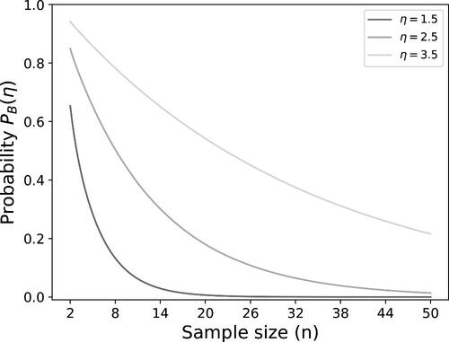
The probability that the observed positive rates for one of the methods is equal to one of the boundaries is given by(8) $$P_B(\eta )=\hspace{0.17em}\text{exp}\hspace{0.17em}\left(-n\eta \right)+{\left(1-\hspace{0.17em}\text{exp}\hspace{0.17em}(-\eta )\right)}^n$$(8) with $\eta =\lambda {\pi }_i$ for measuring microorganism i with the CM and $\eta =\lambda \theta {\pi }_i$ for the RMM. In Figure 1 this probability is visualized as a function of the sample size for three levels of η. It shows that large sample sizes may be needed to have a low probability that the positive rates are away from the boundary, in particular when η is larger.

Fig. 1 Visualization of the probability of observing only positive or only negative test results.

In case m > 1, we may be less stringent on boundary issues when at least one type of microorganism satisfies $0<{\overline{Y}}_{ij}<1$, with $j\in \{1,2\}$. Indeed, when the observed positive rates for one type of microorganism are away from the boundary, this microorganism already provides a proper estimate of θ (and its standard error) and therefore, we may allow the observed positive rates of other types of microorganisms to be equal to the boundary. However, we demonstrate in Appendix A that we still must ignore microorganisms when both observed positive rates are equal to the same boundary (${\overline{Y}}_{i1}={\overline{Y}}_{i2}=1$ or ${\overline{Y}}_{i1}={\overline{Y}}_{i2}=0$) if we wish to obtain proper estimates of θ and π_i (assuming that at least one type of microorganism has data away from the boundaries), but we do not have to exclude data when only one method has an observed positive rate at the boundary.

The $(m+1)\times (m+1)$ Fisher information matrix I is determined by the following moments of the score functions (see Appendix B)(9) $$\begin{array}{ccc}\text{var}(\stackrel{.}{{\mathcal{L}}_{\theta }})& =& \sum _{i=1}^m\frac{n{\lambda }^2{\pi }_i^2\hspace{0.17em}\text{exp}\hspace{0.17em}(-\lambda \theta {\pi }_i)}{1-\hspace{0.17em}\text{exp}\hspace{0.17em}(-\lambda \theta {\pi }_i)}\\ \text{var}({\stackrel{.}{\mathcal{L}}}_{{\pi }_i})& =& n{\lambda }^2\left(\frac{\hspace{0.17em}\text{exp}\hspace{0.17em}(-\lambda {\pi }_i)}{1-\hspace{0.17em}\text{exp}\hspace{0.17em}(-\lambda {\pi }_i)}+\frac{{\theta }^2\hspace{0.17em}\text{exp}\hspace{0.17em}(-\lambda \theta {\pi }_i)}{1-\hspace{0.17em}\text{exp}\hspace{0.17em}(-\lambda \theta {\pi }_i)}\right)\\ \text{cov}(\stackrel{.}{{\mathcal{L}}_{\theta }},{\stackrel{.}{\mathcal{L}}}_{{\pi }_{i1}})& =& \frac{n{\lambda }^2\theta {\pi }_i\hspace{0.17em}\text{exp}\hspace{0.17em}(-\lambda \theta {\pi }_i)}{1-\hspace{0.17em}\text{exp}\hspace{0.17em}(-\lambda \theta {\pi }_i)}\\ \text{cov}({\stackrel{.}{\mathcal{L}}}_{{\pi }_s},{\stackrel{.}{\mathcal{L}}}_{{\pi }_r})& =& 0,r\ne s\end{array}$$(9)

Using the inverse of the Fisher information matrix $I^{-1}$, the asymptotic variance of $\widehat{\theta }$ can be determined in a closed-form expression (see Appendix B) and it is given by(10) $${\tau }_A^2\equiv \text{var}(\widehat{\theta })={\left[\sum _{i=1}^m\frac{n{\lambda }^2{\pi }_i^2}{(\hspace{0.17em}\text{exp}\hspace{0.17em}(\lambda \theta {\pi }_i)-1)+{\theta }^2(\hspace{0.17em}\text{exp}\hspace{0.17em}(\lambda {\pi }_i)-1)}\right]}^{-1}\mathrm{}.$$(10)

An estimate ${\widehat{\tau }}_A^2$ of this asymptotic variance can be obtained by substituting the ML estimators $\widehat{\theta }$ and ${\widehat{\pi }}_i$ in (10). Using this estimated asymptotic variance, an asymptotic one-sided confidence limit can be constructed by(11) $${\text{LCL}}_{\theta }=\widehat{\theta }-z_{1-\alpha }{\widehat{\tau }}_A,$$(11) with α being the significance level and z_q the qth quantile of the standard normal distribution. Then the noninferiority hypothesis (3) is rejected when the lower confidence limit is above the noninferiority margin δ, that is, ${\text{LCL}}_{\theta }>\delta$.

Alternatively, we will use a lower confidence limit on the ML estimator of the logarithmically transformed accuracy $\text{log}\hspace{0.17em}(\theta ),$ with $\text{log}\hspace{0.17em}$ the natural logarithm, since we expect that the distribution of a logarithmic transformation of an estimator of a ratio (see (2)) may converge faster to a normal distribution than the distribution of the ratio estimator itself. The lower confidence limit on the logarithmic transformed estimator can be obtained with the delta method (Cramér 1946), leading to(12) $${\text{LCL}}_{\hspace{0.17em}\text{log}\hspace{0.17em}(\theta )}=\hspace{0.17em}\text{log}\hspace{0.17em}(\widehat{\theta })-z_{1-\alpha }{\widehat{\theta }}^{-1}{\widehat{\tau }}_A.$$(12)

In this case, the noninferiority hypothesis (3) is rejected when this transformed lower confidence limit is above the logarithmically transformed noninferiority margin, that is, ${\text{LCL}}_{\hspace{0.17em}\text{log}\hspace{0.17em}(\theta )}>\hspace{0.17em}\text{log}\hspace{0.17em}(\delta )$. Note that this transformed approach leads to a multiplicative noninferiority test in the original scale of the accuracy and could therefore have a better power than the test based on (11).

2.2 Optimal Spiking Design

For our optimal spiking design, we will focus on an experiment with a single spiked solution for each type of microorganism that is then used to collect 2n samples. Since the detection proportion π_i for microorganism i is typically unknown at the design stage, we would like to determine one optimal level for the mean spike per test sample λ that is used for all microorganisms. In other words, to maximize the power of our noninferiority test in either (11) or in (12), we should minimize the variance ${\tau }_A^2$ in (10) over the mean spike λ, while the detection proportions π₁, π₂, …, π_m are being unknown and potentially arbitrary.

The variance ${\tau }_A^2$ in (10) can be bounded from below and from above using minima and maxima values of the elements in the sum in (10). Indeed, the sum in (10) is smaller than or equal to m times the maximum element and larger than or equal to m times the minimum element. These boundaries only include a single detection proportion, making the form of the variance in (10) somewhat easier to study. The boundaries for the variance ${\tau }_A^2$ are given by$$\begin{array}{c}{\min }_i\left\{\frac{(\hspace{0.17em}\text{exp}\hspace{0.17em}(\lambda \theta {\pi }_i)-1)+{\theta }^2(\hspace{0.17em}\text{exp}\hspace{0.17em}(\lambda {\pi }_i)-1)}{mn{\lambda }^2{\pi }_i^2}\right\}\le {\tau }_A^2\\ \mathrm{\hspace{1em}}\mathrm{\hspace{1em}}\le {\max }_i\left\{\frac{(\hspace{0.17em}\text{exp}\hspace{0.17em}(\lambda \theta {\pi }_i)-1)+{\theta }^2(\hspace{0.17em}\text{exp}\hspace{0.17em}(\lambda {\pi }_i)-1)}{mn{\lambda }^2{\pi }_i^2}\right\}.\end{array}$$

Clearly, the maximum and minimum variance are reached at different values of the detection proportion and the two boundaries will become equal to each other when all detection proportions are equal (${\pi }_1={\pi }_2=\dots ={\pi }_m=\pi$). The variance of the ML estimator $\widehat{\theta }$ then reduces to(13) $$V_E=\frac{(\hspace{0.17em}\text{exp}\hspace{0.17em}(\lambda \theta \pi )-1)+{\theta }^2(\hspace{0.17em}\text{exp}\hspace{0.17em}(\lambda \pi )-1)}{mn{\lambda }^2{\pi }^2}.$$(13)

It can be shown that V_E in (13) is a convex function with respect to π, λ, and $\lambda \pi$ (Appendix C), which implies that it has a unique minimum for λ. However, the solution for λ would depend on the detection proportion π and the accuracy θ and it does not come in a closed-form expression. On the other hand, we know that the optimal solution for λ is of the form $\lambda ={\lambda }_0{\pi }^{-1}$, since the variance in (13) is a function of $\lambda \pi$. The solution of the optimal λ₀ for the minimum variance in (13) can be found by setting the derivative of (13) with respect to $\lambda \pi$ equal to zero, and thus satisfies the following equation(14) $$(\theta {\lambda }_0-2)\hspace{0.17em}\text{exp}\hspace{0.17em}(\theta {\lambda }_0)+{\theta }^2({\lambda }_0-2)\hspace{0.17em}\text{exp}\hspace{0.17em}({\lambda }_0)+2(1+{\theta }^2)=0.$$(14)

Table 1 shows the optimal values λ₀ for different values of accuracy θ using the Newton–Rhapson procedure (Süli and Mayers 2003).

Table 1 Optimal values of λ₀ for different levels of accuracy θ and optimal sample sizes mn for 80% power.

Accuracy (θ)	0.80	0.85	0.90	0.95	1.00
Optimal ${\lambda }_0=\lambda \pi$	1.768	1.721	1.677	1.634	1.594
mn for ${\text{LCL}}_{\theta }$	1232	616	388	276	213
mn for ${\text{LCL}}_{\hspace{0.17em}\text{log}\hspace{0.17em}(\theta )}$	1079	509	303	205	151

The optimal spike λ can be selected approximately when there would be knowledge on the average detection proportion $\overline{\pi }={\sum }_{i=1}^m{\pi }_i/m$ for the CM, because the first-order approximation of ${\sum }_{i=1}^m([n{\lambda }^2{\pi }_i^2]/[\text{exp}\hspace{0.17em}(\lambda \theta {\pi }_i)-1+{\theta }^2(\hspace{0.17em}\text{exp}\hspace{0.17em}(\lambda {\pi }_i)-1)])$ in (10) is equal to $[mn{\lambda }^2{\overline{\pi }}^2]/[\text{exp}\hspace{0.17em}(\lambda \theta \overline{\pi })-1+{\theta }^2(\hspace{0.17em}\text{exp}\hspace{0.17em}(\lambda \overline{\pi })-1)]$. Thus, the first-order approximation of the variance in (10) is given by (13) with the detection proportion π replaced by $\overline{\pi }$. If however information on the (average) detection proportion is lacking, then it should be noted that what is actually needed, is some knowledge on the product $\lambda {\pi }_i$. This can be obtained for a particular organism by performing a pilot experiment in which a laboratory uses a compendial enumeration method to estimate $\widehat{{\lambda }_i}$ of the spike λ for microorganism i, assuming that the detection proportion ${\pi }_i=1$ for the compendial enumeration method. If the latter assumption is not fulfilled, then λ_i actually estimates the product $\lambda {\pi }_i$, which can be used to design the study.

A minimum sample size mn that provides power $1-\beta$ for testing hypothesis (3) using the proposed confidence limit in (11), can be calculated with the well-known sample size formula for a simple hypothesis test based on normality (Donner, Birkett and Buck 1981; Hsieh 1988; Julious 2004)(15) $$\begin{array}{c}mn=\frac{{[z_{1-\alpha }+z_{1-\beta }]}^2[\text{exp}\hspace{0.17em}(\theta {\lambda }_0)-1+{\theta }^2(\hspace{0.17em}\text{exp}\hspace{0.17em}({\lambda }_0)-1)]}{{\lambda }_0^2{\left(\theta -\delta \right)}^2}.\hfill \end{array}$$(15)

When we would use the logarithmically transformed test statistic in (12), the corresponding sample size formula would be equal to (15) with ${(\theta -\delta )}^2$ replaced by ${\theta }^2{(\hspace{0.17em}\text{log}\hspace{0.17em}(\theta )-\hspace{0.17em}\text{log}\hspace{0.17em}(\delta ))}^2$. Since $\text{log}\hspace{0.17em}(1+x)>x{[1+x]}^{-1}$ for all positive x, we obtain that $\text{log}\hspace{0.17em}(\theta )-\hspace{0.17em}\text{log}\hspace{0.17em}(\delta )>1-\delta /\theta$ for all $\theta >\delta$. Hence, the sample size will be smaller for the logarithmically transformed test statistic compared to the nontransformed test statistic when the accuracy is beyond the noninferiority margin. Or in other words, the logarithmically transformed test will have more power than the nontransformed test when applied to the same dataset.

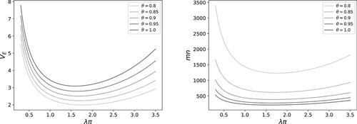
Several sample sizes mn are presented in Table 1 for different values of accuracy θ for a selected noninferiority margin of $\delta =0.7$. It demonstrates that the total sample size can stay below 400 test samples when the true accuracy is at least 0.9 and an optimal spike can be selected. However, the sample sizes are calculated under ideal settings (an optimal spike and equal detection proportions) and it requires an evaluation when the settings would be different in practice. Figure 2 shows that the variance (13) and the sample size (15) may substantially change with the value $\lambda \pi$, especially for values below 1 or above 3, which may be an issue when exact information on the average detection proportion is lacking. In the following section we will conduct simulations to better understand the influence of unequal detection proportions on our testing procedure.

Fig. 2 The variance V_E (with mn = 1) and the sample size mn ($\alpha =0.05$, $\beta =0.20,\delta =0.7$) as a function of $\lambda \pi$ for different values of θ.

3 Simulation

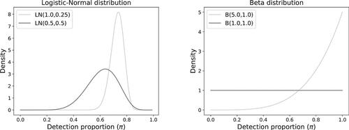
To simulate data for our (optimal) spiking experiment, we need to select different detection proportions for the CM. We will follow two different approaches. First of all, we will assume that the detection proportions are drawn randomly from a probability distribution. This means that for each simulation run we draw a new set of detection proportions. We used the logistic-normal $LN(\mu ,\sigma )$ and the beta B(a, b) distribution. For the logistic-normal distribution, the detection proportion for the CM is set to ${\pi }_i=\hspace{0.17em}\text{exp}\hspace{0.17em}(Z_i)/(1+\hspace{0.17em}\text{exp}\hspace{0.17em}(Z_i))$, with Z_i drawn from a normal distribution, $Z_i\sim N(\mu ,{\sigma }^2)$, and for the beta distribution the detection proportion is set to ${\pi }_i=U_i$, with $U_i\sim B(a,b)$. For both distributions, we used two different settings: $(\mu ,\sigma )=(1,0.25)$ and $(0.5,0.5)$, and $(a,b)=(5,1)$ and (1, 1), respectively. The density functions for these choices of distributions are given in Figure 3. The mean detection proportions $\overline{\pi }$ for these four distributions are equal to 0.73, 0.62, 0.83, and 0.5, respectively. Second, we will consider different sets of fixed detection proportions. For these settings, the proportions will remain the same for each simulation run. One set of detection proportions consists of the quantiles ${\pi }_i=F^{-1}(i/(m+1))$, with F one of the logistic-normal or beta distributions and m the number of microorganisms. The second set of detection proportions consists of a small detection proportion between 0.1 and 0.2 and the other detection proportions above 0.5 such that the average of the detection proportions is equal to the mean detection of one of the four distributions F. For this settings we only consider m = 5 different types of microorganisms. For the distribution $LN(1,0.25)$, the detection proportions are chosen equal to 0.15, 0.75, 0.83, 0.91, and 0.99, with an average of $\overline{\pi }=0.73$. For the distribution $LN(0.5,0.5)$, the detection proportions are chosen equal to 0.15, 0.7, 0.725, 0.75, and 0.775, with an average of $\overline{\pi }=0.62$. For the beta distribution B(5, 1), the detection proportions are selected equal to 0.2, 0.975, 0.983, 0.991, and 0.999 with an average of $\overline{\pi }=0.83$ and, finally, for the distribution B(1, 1) the detection proportions are selected equal to 0.15, 0.5, 0.56, 0.62, and 0.68, with an average of $\overline{\pi }=0.5$.

Fig. 3 Density functions for the simulation of detection proportions (left: logistic-normal; right: beta).

3.1 Simulation of Spiking Experiment

We select different numbers for the types of microorganism ($m\in \{5,10,15\}$) and use three levels for the homogeneous accuracy ($\theta \in \{0.8,0.9,1.0\}$). We also choose $\theta =0.7$ equal to the noninferiority margin $\delta =0.7$ to investigate the Type I error. After selecting m and θ, we draw the detection proportions π₁₁, π₂₁, …, ${\pi }_{m1}$ for the CM using one of the four distributions for the random case. For the fixed setting of detection proportions, we just use the set of values we indicated above. Moreover we determine ${\pi }_{i2}=\theta {\pi }_{i1}$ for the RMM. Then, the sample size n is taken such that mn is equal to the optimal sample size in Table 1 using test statistic ${\text{LCL}}_{\theta }$. In case n would not be an integer we rounded n to the nearest integer value larger than n. Then, for each microorganism i and method j, we simulated the numbers of microorganisms $X_{ij1},X_{ij2}$, …,X_ijn in the n test samples using a Poisson(λ) distribution, with λ being the average number of microorganisms in the test samples ($\lambda \in \{1.5,2.0,2.5,3.0,3.5\}$). These numbers of microorganisms are assumed to be independent. Then, the observed binary outcomes $Y_{ij1},Y_{ij2}$, …, Y_ijn , are independently generated with a Bernoulli distribution using the conditional distribution $\mathbb{P}(Y_{\mathit{ijk}}=1|X_{\mathit{ijk}})=1-{(1-{\theta }_j{\pi }_{i1})}^{X_{\mathit{ijk}}}$, with ${\theta }_j=1$ if j = 1 and ${\theta }_j=\theta$ if j = 2. This procedure is repeated 1000 times, to obtain multiple simulated spiking experiments under the same settings and investigate the power of our test statistics. The simulation of this spiking experiment was conducted with SAS software, version 9.4.

3.2 Analysis of Simulated Spiking Experiment

For each simulated dataset, we calculated the observed positive rate ${\overline{Y}}_{ij}$ for microorganism i and method j. To be able to estimate the parameters θ and π_i and to conduct the noninferiority tests for each simulated spiking experiment, we first had to clean the data and eliminate types of microorganisms with observed positive rates at the boundary. Any type of microorganism with either only negative (${\overline{Y}}_{i1}={\overline{Y}}_{i2}=0$) or otherwise only positive samples (${\overline{Y}}_{i1}={\overline{Y}}_{i2}=1$) were removed from the data when we had at least one type of microorganism with data $0<{\overline{Y}}_{ij}<1$ (Appendix A). Information on the number of microorganisms that were available for the analysis will be reported.

It is expected that the detection proportions that are randomly drawn for each simulation run will typically result in less extreme results than for the fixed settings. The reason is that in the fixed settings several proportions are really close to one (especially for the distributions B(5, 1) and $LN(1.0,0.25)$), which may result in positive rates for microorganisms equal to the boundary one for the corresponding microorganisms. Thus, the consequence is that more datasets may be eliminated in the fixed settings compared to the random settings.

After eliminating microorganisms, the model parameters are estimated and the noninferiority tests are performed. In practice, laboratories are often able to provide an estimate ${\widehat{\lambda }}_i$ of the spike λ for microorganism i using a compendial enumeration method. This estimate can be used in the analysis by substituting λ by this estimate. In the simulation study we used ${\widehat{\lambda }}_i=[{\overline{X}}_{i1}+{\overline{X}}_{i2}]/2$ as proxy, with ${\overline{X}}_{ij}={\sum }_{k=1}^n{X}_{\mathit{ijk}}/n$ the simulated average in the test sample. The analysis of the data was conducted with SAS software, version 9.4, using procedure NLMIXED. Both the Type I error and the power of the noninferiority test will be reported.

3.3 Simulation Results

In this section, we only report the results of the detection proportions that were drawn randomly from the four distributions for each simulation run. The results of the fixed detection proportions are reported in Appendix D. The conclusions for these different ways of selecting detection proportions are not fundamentally different. The Type I error rates between these two approaches are very comparable, but the power values are somewhat lower in the fixed settings for higher values of the spike level λ. This can be fully explained by the higher numbers of datasets that must be eliminated (as we described in Appendix A). Our sample sizes are calculated under the assumption that none of the data is being eliminated. Thus, if then substantial amounts of data must be removed because they cannot contribute to the estimation of the parameters, the sample sizes have been underestimated, leading to lower powers that may drop below 80%.

Table 2 shows the average, the minimum, the maximum, and the 5% quantile of the numbers of microorganisms that were not removed from the simulated spiking experiment (m = 15, $\lambda =3.5$) for the four distributional choices and for two levels of accuracy. For the other chosen settings, all with lower m, λ, and θ, less data had to be removed since these settings had a lower chance of obtaining boundary values (see (8)).

Table 2 Summary statistics of the included number of microorganisms for random detection proportions.

Distribution	$\theta =0.9$				$\theta =1.0$
	Mean	Min	Max	$q_{0.05}$	Mean	Min	Max	$q_{0.05}$
$LN(1,0.25)$	14.85	11	15	14	13.61	10	15	12
$LN(0.5,0.5)$	14.94	13	15	14	14.34	11	15	13
B(5,  1)	14.16	10	15	13	11.77	6	15	9
B(1,  1)	14.69	11	15	14	13.80	7	15	12

It shows that it is unlikely to remove more than 6 types of microorganisms in a spiking experiment with 15 microorganisms (i.e., a quantile of 9 for distribution B(5, 1)), but in most settings it is expected to remove substantially less data. Clearly, the relative small sample size of n = 15, calculated for an accuracy of θ = 1, is more likely to provide data at the boundaries frequently when the average spike would be larger (see (8) and Figure 1), but this is less of an issue when the sample size is larger and the accuracy is smaller, for example, when n = 26 and $\theta =0.9$.

The performance of the two noninferiority tests is provided in Figures 4–7. Figure 4 provides the simulated Type I error rate, while the other three figures provide the power of the tests for different levels of accuracy (at significance $\alpha =0.05$). In each figure we show the results of the four choices of distribution functions for the detection proportions and the three settings for the number of microorganisms ($m\in \{5,10,15\}$) with the corresponding sample sizes n.

Fig. 4 Type I error rate of the two noninferiority test ($\theta =0.7$) as a function of λ for different distributions and number of microorganisms when detection proportions are selected randomly.

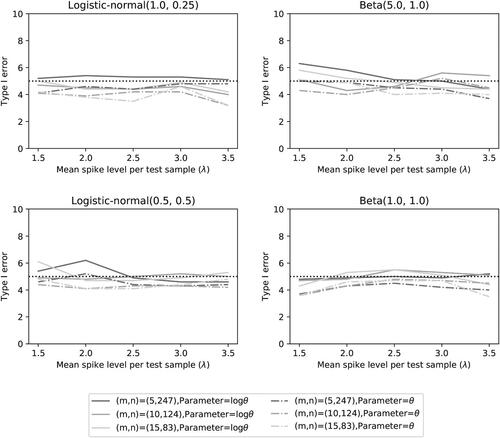
Fig. 5 Power of the two noninferiority tests ($\theta =0.8$) as a function of λ for different distributions and number of microorganisms when detection proportions are selected randomly.

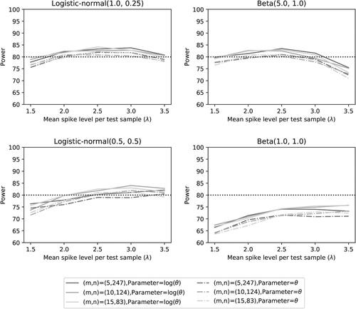
Fig. 6 Power of the two noninferiority tests ($\theta =0.9$) as a function of λ for different distributions and number of microorganisms when detection proportions are selected randomly.

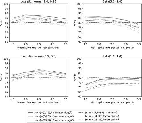
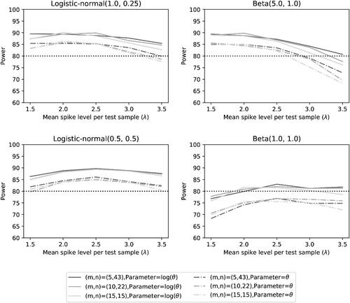
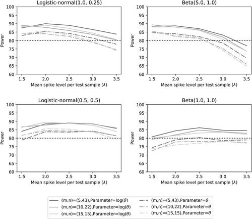
Fig. 7 Power of the two noninferiority tests (θ = 1) as a function of λ for different distributions and number of microorganisms when detection proportions are selected randomly.

Figure 4 shows that the significance level of 5% is nicely achieved. This may not be a surprise, since we used a sample size mn that was calculated under assumption that the accuracy is equal to $\theta =0.7$. The fluctuations of the Type I error rates seem to be random and unrelated to the choices of distributions.

The results on power demonstrate that the noninferiority test ${\text{LCL}}_{\hspace{0.17em}\text{log}\hspace{0.17em}(\theta )}$ is more powerful than ${\text{LCL}}_{\theta }$ (as expected). For the first three distributions, a power of 80% is achieved for ${\text{LCL}}_{\hspace{0.17em}\text{log}\hspace{0.17em}(\theta )}$ in most settings when the average spike λ can be maintained within 2 to 3 colony forming units per test sample (CFU/sample). This does not always occur for test ${\text{LCL}}_{\theta }$, even though we used the sample size calculation for this test. Spiking levels at $\lambda =1.5$ and/or $\lambda =3.5$ CFU/sample may diminish the power, depending on the mean detection proportion of the distribution in combination with the accuracy. Indeed, the distributions with lower mean detection proportions ($LN(0.5,0.5$) and B(1, 1)) seem to benefit from a somewhat higher spike, in particular when the accuracy is lower. This is not surprising since the first-order approximation of variance ${\tau }_A^2$ in (10) is equal to V_E in (13) with π replaced by $\overline{\pi }$ (see Section 2.2). The two distributions with a higher mean detection proportion seem to do better for lower spike levels, but a level of 1.5 CFU/sample still seems to be too low. This is not surprising either, since a spike lower than 1.593 would be less optimal even when the mean detection proportion would be equal to one (see Table 1).

A power of 80% does not seem to be attained for any spike level when the accuracy is $\theta =0.8$ and the detection proportions follow a uniform distribution (B(1, 1)). We think this may be caused by detection proportions close to zero. The variance V_E for the accuracy estimator for detection proportions close to zero would have extreme standard errors (see Figure 2). Thus, just one small detection proportion may affect the power of the test negatively. For lower values of θ this effect is enhanced compared to accuracies closer to one.

The form of the density for the detection proportions also seems to affect the power of the noninferiority test on accuracy, which is probably caused by the likelihood of a small detection proportion. The distributions $LN(0.5,0.5)$ and B(1, 1) do not just have a lower mean, they also show more variability, with a higher probability of generating small detection proportions. Based on our past experiences with the CM, we expect that the $LN(1.0,0.25)$ and $B(5.0,1.0)$ are more realistic distributions on detection proportions in practice than the other two. Having detection proportions below 0.3 for microorganisms with the CM seems less likely, unless the microorganism is highly stressed and unwilling to grow.

4 Case Study

Our approach has been implemented in practice, where a specific RMM was compared to the CM. The company who performed the validation study decided to test m = 16 different types of microorganism and used noninferiority margin $\delta =0.7$. Although there is no reason to assume that the RMM is inferior to the CM, the accuracy will be considered less than 1 to avoid being too optimistic. It was assumed that the accuracy was in the range $\theta \in [0.85,0.95]$. This leads to a sample size in the range of $n\in [18,39]$, using test statistic ${\text{LCL}}_{\theta }$ and Table 1. It was therefore decided to take n = 30 test samples per microorganism and method, allowing for a true accuracy of just below 0.9. The optimal λ₀ should be chosen between 1.634 and 1.721 CFU/sample. Assuming that the mean detection proportion may be close to 0.5, since a few difficult to test microorganisms are being tested, a spike λ in the range of 3 CFU/sample was recommended.

The collected number of positive test samples for the noninferiority study are given in Table 3. The company also provided an estimated or predicted spike level based on the compendial enumeration method.

Table 3 Numbers of positive test samples out of 30 test samples from a real noninferiority study.

Microorganism	$Y_{i1.}$	$Y_{i2.}$	${\widehat{\lambda }}_i$	Microorganism	$Y_{i1.}$	$Y_{i2.}$	${\widehat{\lambda }}_i$
E.coli	28	28	2.16	C.sporogenes	13	16	0.50
C.albicans	25	24	1.67	A.lwoffi	1	1	0.33
S.aureus	30	29	2.67	S.pyogenes	25	24	2.67
B.cereus	29	28	3.67	S.maltophilia	28	26	4.50
P.aeruginosa	20	16	1.00	K.rhizophila	30	26	2.00
B.cepacia	8	8	0.16	C.acnes	26	22	3.33
S.warneri	3	4	1.16	P.chrysogenum	1	1	1.50
B.subtilis	26	28	2.83	A.brasiliensis	27	27	1.50

The model and methodology as explained in Section 2 was used to estimate the accuracy and the detection proportions for all microorganisms with the CM. We used the estimated spike levels provided by the company in the analysis, but we obtained the same conclusion on the accuracy when we ignored this information. If the estimated spike would be somewhat too low (or underestimated), we would obtain estimates for the detection proportions that may be larger than one. This is not an issue when interest is in the estimation and testing of the accuracy, it merely shows that the predicted spike level was not accurately determined. The SAS code is provided in Appendix E.

The estimates of the individual detection proportions and their 95% confidence intervals are given in Table 4. The estimate of the logarithmically transformed accuracy with its 90% confidence interval is given by –0.156 $[-0.319,0.007]$. Since the noninferiority margin in the log scale is equal to $-0.357\approx \hspace{0.17em}\text{log}\hspace{0.17em}(0.7)$, we reject the null hypothesis on inferiority and conclude that the RMM is most likely noninferior to the CM. The estimate of the accuracy with its 90% confidence interval is $\widehat{\theta }=0.856$ $[0.727,1.007]$.

Table 4 Estimated detection proportions with their 95% confidence intervals.

Microorganism	πi	LCL	UCL	Microorganism	πi	LCL	UCL
E.coli	1.36	0.86	1.85	C.sporogenes	1.42	0.88	1.96
C.albicans	1.10	0.74	1.46	A.lwoffi	0.11	0.00	0.26
S.aureus	1.70	0.84	2.55	S.pyogenes	0.69	0.46	0.91
B.cereus	0.89	0.55	1.23	S.maltophilia	0.56	0.36	0.75
P.aeruginosa	0.99	0.64	1.34	K.rhizophila	1.50	0.93	2.07
B.cepacia	2.09	1.04	3.13	C.acnes	0.53	0.35	0.70
S.warneri	0.12	0.03	0.20	P.chrysogenum	0.02	0.00	0.06
B.subtilis	0.87	0.58	1.17	A.brasiliensis	1.66	1.09	2.23

5 Discussion and Conclusion

We have provided an optimal framework for a noninferiority study on detection of microorganisms between two qualitative microbiological methods where we have assumed that the accuracy or recovery parameter is homogeneous across all types of microorganisms. We provided the optimal average spike level for the test samples taken from a single solution experiment and presented a sample size formula. Our simulation study showed that the proposed noninferiority tests have a power that is close to or better than the requested power. We recommend to use the logarithmically transformed accuracy test in the analysis, but a sample size calculation that is conducted for the accuracy test in the original scale. The reason for this discrepancy is that our calculations are somewhat optimistic since they are calculated under ideal circumstances.

The main benefit of our approach is the potential of a substantial reduction in sample sizes. IJzerman-Boon and Van denHeuvel (2015) showed that a sample size of 200 test samples per microbiological method for one microorganism is necessary to obtain 80% power for a traditional hypothesis test on accuracy when the true accuracy is 70%. For a homogeneous accuracy setting, this number could theoretically be reduced to 213 test samples for all microorganisms together, when the number of microorganisms is limited to 7. The reason for this limit is that with less than 30 test samples per microorganism, there is a risk that the collected data on a microorganism is not suitable for noninferiority testing, because the positive rates likely become equal to zero or one, excluding this microorganism from participating in the noninferiority study. Our case study demonstrated that a sample size of 30 test samples per method for each microorganism is attainable and worked nicely and we recommend not to go lower due to this risk of observing boundary values. This is still a reduction in sample sizes of about 85% with current status quo.

Our analysis also demonstrated that an optimal average spike is somewhere in between 2 and 3 CFU/sample when the detection proportions are larger than 0.5 and not all equal to one. This is in line with the official guidelines (USP < 1223 > 2015), who propose to choose a spike level such that the positive rate for the compendial is between 50 to 75%, even though higher spike levels have been recommended in the past. However, our noninferiority test is different from these guidelines, which proposes to use the most probable number (MPN) that is calculated from multiple dilutions or a noninferiority test on the positive rates. The MPN is less powerful than our test statistic and the second test statistic is highly sensitive to the spike and may falsely result in noninferiority when spike levels are selected somewhat higher (IJzerman-Boon, Manju, and Van denHeuvel 2020).

The disadvantage of our approach is that it is not known whether we may assume a homogeneous accuracy in practice. When the rapid and the compendial method have the same detection principles or mechanisms, but the rapid method is just faster than the compendial method in establishing a decision, it may not be unrealistic that there exists a consistent ratio between the two methods on detecting a single organism across different types of microorganisms. However, when detection mechanisms between the rapid and compendial method are truly different it is unknown if a common accuracy is realistic. Note that different detection proportions for detecting different organisms can be assumed for a common or homogeneous accuracy as well as for heterogeneous accuracies. In case the assumption of a common accuracy is false or there exists doubt on the assumption, different microorganisms may possibly be grouped based on their expectation of equal accuracy, but with different accuracies across groups. If certain groups can be formed, then our noninferiority framework can be applied to these groups separately and still result in lower sample sizes. In the near future, we are planning to study statistical tests that could evaluate the assumption of a homogeneous accuracy or otherwise determine the influence of heterogeneous accuracies on the noninferiority of the rapid method compared to the compendial method for a particular organism. This may complement the work we provided here. It should be noted that in the presented case study the likelihood ratio test for testing the null hypothesis of one common accuracy was not rejected (p = 0.794), suggesting that homogeneity of accuracy was reasonable, but the power (and Type I error) of the likelihood ratio test still need evaluation.

Additional information

Funding

This work is part of the research program Rapid Micro Statistics with project number 15990, which is (partly) financed by the Dutch Research Council (NWO).

Notes

1 This equation actually has a solution whenever the observed positive rates ${\overline{Y}}_{21}$ and ${\overline{Y}}_{22}$ are not equal to the same boundary value as we will see for the second equation in (A.1) in Scenarios 2 to 5. Thus, one of the positive rates is allowed to be equal to the boundary, as long as the other is not. However, characteristics of the solution depend on whether or not the positive rates are at a boundary zero or not.

Appendix A

Here, we discuss maximum likelihood estimation of the model parameters θ and π₁, π₂, …, π_m for model (4) based on data $\left\{Y_{\mathit{ijk}}\right\}$, where part of the data may be at the boundary value (${\overline{Y}}_{ij}\in \{0,1\}$), but at least one type of microorganism has data that is not at the boundary ($0<{\overline{Y}}_{ij}<1$, $j\in \{1,2\}$). We illustrate this for just two microorganisms, where one microorganism may have observed boundary values (i = 1) and the other microorganism has not (i = 2). We may assume λ = 1, because we could just replace $\lambda {\pi }_i$ by a new parameter η_i that should be estimated instead. The likelihood equations from (6) are then reduced to the following three equations:(A.1) $$\begin{array}{ccc}{\pi }_1{\overline{Y}}_{12}{[1-\hspace{0.17em}\text{exp}\hspace{0.17em}\{-\theta {\pi }_1\left\}\right]}^{-1}+{\pi }_2{\overline{Y}}_{22}{[1-\hspace{0.17em}\text{exp}\hspace{0.17em}\{-\theta {\pi }_2\left\}\right]}^{-1}& =& {\pi }_1+{\pi }_2,\\ {\overline{Y}}_{11}{[1-\hspace{0.17em}\text{exp}\hspace{0.17em}\{-{\pi }_1\left\}\right]}^{-1}+\theta {\overline{Y}}_{12}{[1-\hspace{0.17em}\text{exp}\hspace{0.17em}\{-\theta {\pi }_1\left\}\right]}^{-1}& =& 1+\theta ,\\ {\overline{Y}}_{21}{[1-\hspace{0.17em}\text{exp}\hspace{0.17em}\{-{\pi }_2\left\}\right]}^{-1}+\theta {\overline{Y}}_{22}{[1-\hspace{0.17em}\text{exp}\hspace{0.17em}\{-\theta {\pi }_2\left\}\right]}^{-1}& =& 1+\theta .\end{array}$$(A.1)

The proof is built up in the following way. First, we demonstrate that the MLE’s do not exist when ${\overline{Y}}_{11}$ and ${\overline{Y}}_{12}$ are at the same boundary. For all remaining settings the MLE’s do exist. To demonstrate that claim, we first discuss the solution ${\widehat{\pi }}_2(\theta )$ for π₂ using the third equation in (A.1). We show its existence for each θ and study ${\widehat{\pi }}_2(\theta )$ as function of θ, to determine certain characterizations we need later in the proof. Then we study ${\widehat{\pi }}_1(\theta )$ in the second equation of (A.1) for different data scenarios of ${\overline{Y}}_{11}$ and ${\overline{Y}}_{12}$. In these scenarios we also study the solution $\widehat{\theta }$ for the first equation in (A.1) when the solutions ${\widehat{\pi }}_1(\theta )$ and ${\widehat{\pi }}_2(\theta )$ are substituted.

The same boundary values for the first microorganism

In case ${\overline{Y}}_{11}=0$ and ${\overline{Y}}_{12}=0$, the second equation in (A.1) reduces to $0=\theta +1$, which results in the unrealistic estimator of $\widehat{\theta }=-1$. When ${\overline{Y}}_{11}=1$ and ${\overline{Y}}_{12}=1$, the second equation in (A.1) becomes equal to ${[\text{exp}\hspace{0.17em}\{{\pi }_1\}-1]}^{-1}+\theta {[\text{exp}\hspace{0.17em}\{\theta {\pi }_1\}-1]}^{-1}=0$, which has no finite solution for the detection proportion π₁. Thus, it is obvious that a microorganism can not have two observed positive rates at the same boundary. Therefore, microorganisms with either ${\overline{Y}}_{11}=0$ and ${\overline{Y}}_{12}=0$ or ${\overline{Y}}_{11}=1$ and ${\overline{Y}}_{12}=1$ should be removed from the spiking experiment. For all other settings we will demonstrate that the set of equations in (A.1) has solutions for θ, π₁, and π₂.

Solution detection proportion for the second microorganism

The third equation in (A.1) has a unique solution for π₂ when the observed positive rates satisfy $0<{\overline{Y}}_{21}<1$ and $0<{\overline{Y}}_{22}<1$ and when $\theta >0$ is fixed1. The function ${\overline{Y}}_{21}{[1-\hspace{0.17em}\text{exp}\hspace{0.17em}\{-{\pi }_2\}]}^{-1}+\theta {\overline{Y}}_{22}{[1-\hspace{0.17em}\text{exp}\hspace{0.17em}\{-\theta {\pi }_2\}]}^{-1}$ is a continuous decreasing function in ${\pi }_2>0$, since both parts are decreasing functions. It converges to $\infty$ when π₂ converges to 0 and when π₂ converges to $\infty$, the function converges to ${\overline{Y}}_{21}+\theta {\overline{Y}}_{22}<1+\theta$. Thus, there is just one unique solution ${\widehat{\pi }}_2(\theta )>0$ that solves the third equation in (A.1). It should be noted that ${\widehat{\pi }}_2(1)=-\hspace{0.17em}\text{log}\hspace{0.17em}(1-{\overline{Y}}_2)$, with ${\overline{Y}}_2=[{\overline{Y}}_{21}+{\overline{Y}}_{22}]/2$. Hence, if both methods are equal, that is, θ = 1, then the detection proportion π₂ for the second microorganism is estimated based on the average positive rates ${\overline{Y}}_2$ of the two methods.

Due to the continuity of the function ${\overline{Y}}_{21}{[1-\hspace{0.17em}\text{exp}\hspace{0.17em}\{-{\pi }_2\}]}^{-1}+\theta {\overline{Y}}_{22}{[1-\hspace{0.17em}\text{exp}\hspace{0.17em}\{-\theta {\pi }_2\}]}^{-1}$ in π₂ and θ, the function ${\widehat{\pi }}_2(\theta )$ is continuous in θ. Furthermore, when θ converges to zero, $\theta {\overline{Y}}_{22}{[1-\hspace{0.17em}\text{exp}\hspace{0.17em}\{-\theta {\pi }_2\}]}^{-1}$ would converge to infinity when π₂ would be fixed. Thus, π₂ needs to increase to compensate for this increase and to become or maintain a solution for the third equation in (A.1). This leads to $\underset{\theta \downarrow 0}{\lim }{\widehat{\pi }}_2(\theta )=\infty$ and $\underset{\theta \downarrow 0}{\lim }{\overline{Y}}_{21}{[1-\hspace{0.17em}\text{exp}\hspace{0.17em}\{-{\pi }_2\}]}^{-1}={\overline{Y}}_{21}$. Furthermore, we obtain that $\underset{\theta \downarrow 0}{\lim }\theta {\widehat{\pi }}_2(\theta )=0$, from the observation that$$\underset{\theta \downarrow 0}{\lim }\theta {\overline{Y}}_{22}{[1-\hspace{0.17em}\text{exp}\hspace{0.17em}\{-\theta {\widehat{\pi }}_2(\theta )\left\}\right]}^{-1}=1-{\overline{Y}}_{21}>0,$$after rewriting the third inequality in (A.1).

We will now demonstrate that ${\theta }_0{\widehat{\pi }}_2({\theta }_0)<{\theta }_1{\widehat{\pi }}_2({\theta }_1)$ when $0<{\theta }_0<{\theta }_1$. We only need to address the situation where ${\widehat{\pi }}_2({\theta }_0)\ge {\widehat{\pi }}_2({\theta }_1)$, since otherwise ${\theta }_0{\widehat{\pi }}_2({\theta }_0)<{\theta }_1{\widehat{\pi }}_2({\theta }_1)$ is trivially obtained. When ${\widehat{\pi }}_2({\theta }_0)\ge {\widehat{\pi }}_2({\theta }_1)$ is true, we obtain the following inequality(A.2) $$1-{\overline{Y}}_{21}{[1-\hspace{0.17em}\text{exp}\hspace{0.17em}\{-{\widehat{\pi }}_2({\theta }_0)\left\}\right]}^{-1}\ge 1-{\overline{Y}}_{21}{[1-\hspace{0.17em}\text{exp}\hspace{0.17em}\{-{\widehat{\pi }}_2({\theta }_1)\left\}\right]}^{-1},$$(A.2) since ${[1-\hspace{0.17em}\text{exp}\hspace{0.17em}\{-{\pi }_2\}]}^{-1}$ is a decreasing function in π₂. Now assume that also the alternative inequality ${\theta }_0{\widehat{\pi }}_2({\theta }_0)\ge {\theta }_1{\widehat{\pi }}_2({\theta }_1)$ is true, then we would obtain the inequality(A.3) $${\overline{Y}}_{22}{[1-\hspace{0.17em}\text{exp}\hspace{0.17em}\{-{\theta }_0{\widehat{\pi }}_2({\theta }_0)\left\}\right]}^{-1}-1\le {\overline{Y}}_{22}{[1-\hspace{0.17em}\text{exp}\hspace{0.17em}\{-{\theta }_1{\widehat{\pi }}_2({\theta }_1)\left\}\right]}^{-1}-1,$$(A.3) again using that ${[1-\hspace{0.17em}\text{exp}\hspace{0.17em}\{-{\pi }_2\}]}^{-1}$ is a decreasing function in π₂. Rewriting the third equation in (A.1) as$$\theta =(1-{\overline{Y}}_{21}{[1-\hspace{0.17em}\text{exp}\hspace{0.17em}\{-{\widehat{\pi }}_2(\theta )\left\}\right]}^{-1})/({\overline{Y}}_{22}{[1-\hspace{0.17em}\text{exp}\hspace{0.17em}\{-\theta {\widehat{\pi }}_2(\theta )\left\}\right]}^{-1}-1),$$ and using inequalities (A.2) and (A.3), we obtain the following contradiction:$$\begin{array}{c}{\theta }_0=\frac{1-{\overline{Y}}_{21}{[1-\hspace{0.17em}\text{exp}\hspace{0.17em}\{-{\pi }_2({\theta }_0)\left\}\right]}^{-1}}{{\overline{Y}}_{22}{[1-\hspace{0.17em}\text{exp}\hspace{0.17em}\{-{\theta }_0{\pi }_2({\theta }_0)\left\}\right]}^{-1}-1}\\ \ge \frac{1-{\overline{Y}}_{21}{[1-\hspace{0.17em}\text{exp}\hspace{0.17em}\{-{\pi }_2({\theta }_1)\left\}\right]}^{-1}}{{\overline{Y}}_{22}{[1-\hspace{0.17em}\text{exp}\hspace{0.17em}\{-{\theta }_1{\pi }_2({\theta }_1)\left\}\right]}^{-1}-1}={\theta }_1.\end{array}$$

Thus, $\theta {\widehat{\pi }}_2(\theta )$ must be an increasing function in θ.

Finally, rewriting the third equation and letting θ converge to infinity, we obtain(A.4) $$\underset{\theta \to \infty }{\lim }\frac{{\overline{Y}}_{22}}{1-\hspace{0.17em}\text{exp}\hspace{0.17em}\{-\theta {\widehat{\pi }}_2(\theta )\}}-1=\underset{\theta \to \infty }{\lim }\frac{1}{\theta }\left(1-\frac{{\overline{Y}}_{21}}{1-\hspace{0.17em}\text{exp}\hspace{0.17em}\{-{\widehat{\pi }}_2(\theta )\}}\right).$$(A.4)

Since $\theta {\widehat{\pi }}_2(\theta )$ is an increasing function in θ, it either converges to infinity or to some finite value. In both cases the left-hand side in (A.4) is a finite value. Thus, the right-hand side in (A.4) must be a finite value too. If we define ${\xi }_2=\underset{\theta \to \infty }{\lim }(1-{\overline{Y}}_{21}{[1-\hspace{0.17em}\text{exp}\hspace{0.17em}\{-{\widehat{\pi }}_2(\theta )\}]}^{-1})/\theta$ as this finite limit, we obtain that $\underset{\theta \to \infty }{\lim }\theta {\widehat{\pi }}_2(\theta )=-\hspace{0.17em}\text{log}\hspace{0.17em}(1-{\overline{Y}}_{22}/[1+{\xi }_2])$, with ${\xi }_2\in [{\overline{Y}}_{22}-1,0)$. Note that ξ₂ can not be equal to zero. To demonstrate this, lets assume ${\xi }_2=0$. In this case, we would have that the expression on the left-hand side in (A.4) would be positive for any value of θ, since $\theta {\widehat{\pi }}_2(\theta )$ is an increasing function, ${[1-\hspace{0.17em}\text{exp}\hspace{0.17em}\{-\theta {\widehat{\pi }}_2(\theta )\}]}^{-1}$ is a decreasing function, and its limit is equal to zero. Thus, the expression in the left-hand side of (A.4) approaches ${\xi }_2=0$ from above. We would also have that $\underset{\theta \to \infty }{\lim }{\widehat{\pi }}_2(\theta )=\underset{\theta \to \infty }{\lim }-{\theta }^{-1}\hspace{0.17em}\text{log}\hspace{0.17em}(1-{\overline{Y}}_{22})=0$, since ${\overline{Y}}_{22}<1$. In combination with the fact that $\underset{\theta \downarrow 0}{\lim }{\widehat{\pi }}_2(\theta )=\infty$, this means that we can find a value θ such that the expression on the right-hand side in (A.4) becomes negative, since ${\overline{Y}}_{21}>0$. Since the equality in (A.4) should hold for any value of θ and not just for the limits, we have created a contradiction. Thus, the value ξ₂ must be negative.

Solution detection proportion for the first microorganism

We will now study the solution π₁ from the second equation in (A.1) as a function of θ, assuming that ${\overline{Y}}_{11}$ and ${\overline{Y}}_{12}$ are not both equal to the same boundary. We will make use of the same reasoning as for π₂ where possible. We will study the different settings for ${\overline{Y}}_{11}$ and ${\overline{Y}}_{12}$ and show that the first equation in (A.1) also has a solution in $\widehat{\theta }$ after we substituted the solutions ${\widehat{\pi }}_1(\theta )$ and ${\widehat{\pi }}_2(\theta )$ in the first equation of (A.1).

Scenario 1 {$0<{\overline{Y}}_{11}<1,0<{\overline{Y}}_{12}<1$}

This is the exact same situation as for π₂ and we thus obtain the same characteristics for ${\widehat{\pi }}_1(\theta )$ as for ${\widehat{\pi }}_2(\theta )$. Since ${[1-\hspace{0.17em}\text{exp}\hspace{0.17em}\{-\theta {\widehat{\pi }}_i(\theta )\}]}^{-1}$ converges to infinity when θ converges to zero (since $\underset{\theta \downarrow 0}{\lim }\theta {\widehat{\pi }}_i(\theta )=0$), we can find a value θ₀ such that ${\overline{Y}}_{i2}{[1-\hspace{0.17em}\text{exp}\hspace{0.17em}\{-{\theta }_0{\widehat{\pi }}_i({\theta }_0)\}]}^{-1}>1$ for $i\in \{1,2\}$. For this value, it follows for the left-hand side of the first equation in (A.1) that(A.5) $$\frac{{\widehat{\pi }}_1({\theta }_0){\overline{Y}}_{12}}{1-\hspace{0.17em}\text{exp}\hspace{0.17em}\{-{\theta }_0{\widehat{\pi }}_1({\theta }_0)\}}+\frac{{\widehat{\pi }}_2({\theta }_0){\overline{Y}}_{22}}{1-\hspace{0.17em}\text{exp}\hspace{0.17em}\{-{\theta }_0{\widehat{\pi }}_2({\theta }_0)\}}>{\widehat{\pi }}_1({\theta }_0)+{\widehat{\pi }}_2({\theta }_0).$$(A.5)

Additionally, similar to (A.4) for the second microorganism, ${\overline{Y}}_{i2}{[1-\hspace{0.17em}\text{exp}\hspace{0.17em}\{-\theta {\widehat{\pi }}_i(\theta )\}]}^{-1}$ converges to $1+{\xi }_i<1$ when θ converges to infinity. Thus, we can find a θ₁ such that we have the opposite inequality in (A.5). This implies that there exists a $\theta \in ({\theta }_0,{\theta }_1)$ that would give equality in (A.5), since ${\widehat{\pi }}_i(\theta )$ is a continuous function in θ.

Scenario 2 {${\overline{Y}}_{11}=0,{\overline{Y}}_{12}>0$}

The second equation in (A.1) becomes equal to $\theta {\overline{Y}}_{12}{[1-\hspace{0.17em}\text{exp}\hspace{0.17em}\{-\theta {\pi }_1\}]}^{-1}=1+\theta$ and leads immediately to the solution of ${\widehat{\pi }}_1(\theta )=-{\theta }^{-1}\hspace{0.17em}\text{log}\hspace{0.17em}(1-\theta {\overline{Y}}_{12}/(\theta +1))$. This solution satisfies the same characteristics as the solution from Scenario 1. Indeed, $\theta {\widehat{\pi }}_1(\theta )=-\hspace{0.17em}\text{log}\hspace{0.17em}(1-\theta {\overline{Y}}_{12}/(\theta +1))$ is an increasing function in θ with $\underset{\theta \downarrow 0}{\lim }\theta {\widehat{\pi }}_1(\theta )=0$ and $\underset{\theta \to \infty }{\lim }\theta {\widehat{\pi }}_1(\theta )=-\hspace{0.17em}\text{log}\hspace{0.17em}(1-{\overline{Y}}_{12})$, which could be infinite when ${\overline{Y}}_{12}=1$. Furthermore, the solution ${\widehat{\pi }}_1(\theta )$ converges to infinity when θ converges to zero. To demonstrate the existence of θ, we can use the same reasoning as in Scenario 1. There is again a θ₀ such that inequality in (A.5) holds true, making use of $\underset{\theta \downarrow 0}{\lim }\theta {\widehat{\pi }}_i(\theta )=0,{\overline{Y}}_{i2}>0$, and $1-\hspace{0.17em}\text{exp}\hspace{0.17em}\{-\theta {\widehat{\pi }}_i(\theta )\}$ converges to zero when θ converges to zero. There also exists a ${\theta }_1>{\theta }_0$ such that the inequality in (A.5) is reversed when θ₀ is replaced by θ₁. Indeed, ${\overline{Y}}_{22}{[1-\hspace{0.17em}\text{exp}\hspace{0.17em}\{-\theta {\widehat{\pi }}_2(\theta )\}]}^{-1}$ converges to $1+{\xi }_2<1$ and ${\overline{Y}}_{12}{[1-\hspace{0.17em}\text{exp}\hspace{0.17em}\{-\theta {\widehat{\pi }}_1(\theta )\}]}^{-1}$ converges to 1.

Scenario 3 {${\overline{Y}}_{11}>0,{\overline{Y}}_{12}=0$}

The second equation in (A.1) becomes equal to ${\overline{Y}}_{11}{[1-\hspace{0.17em}\text{exp}\hspace{0.17em}\{-\theta {\pi }_1\}]}^{-1}=1+\theta$ and leads immediately to the solution of ${\widehat{\pi }}_1(\theta )=-\hspace{0.17em}\text{log}\hspace{0.17em}(1-{\overline{Y}}_{11}/(\theta +1))$. This solution is somewhat different from the solution in Scenario 1, since $\underset{\theta \downarrow 0}{\lim }{\widehat{\pi }}_1(\theta )=-\hspace{0.17em}\text{log}\hspace{0.17em}(1-{\overline{Y}}_{11})<\infty$ due to ${\overline{Y}}_{11}>0$. Furthermore, we have that $\theta {\widehat{\pi }}_1(\theta )=-\theta \hspace{0.17em}\text{log}\hspace{0.17em}(1-{\overline{Y}}_{11}/(\theta +1))$ is an increasing function in θ with $\underset{\theta \downarrow 0}{\lim }\theta {\widehat{\pi }}_1(\theta )=0$ but with $\underset{\theta \to \infty }{\lim }\theta {\widehat{\pi }}_1(\theta )=\infty$. We now need to show that there exists a solution θ such that(A.6) $${\overline{Y}}_{22}{[1-\hspace{0.17em}\text{exp}\hspace{0.17em}\{-\theta {\widehat{\pi }}_2(\theta )\left\}\right]}^{-1}=1+{\widehat{\pi }}_1(\theta )/{\widehat{\pi }}_2(\theta ).$$(A.6)

Since ${\widehat{\pi }}_1(0)$ is finite, ${\widehat{\pi }}_2(\theta )$ converges to infinity when θ converges to zero, and $1-\hspace{0.17em}\text{exp}\hspace{0.17em}\{-\theta {\widehat{\pi }}_2(\theta )\}$ converges to zero when θ converges to zero, we can select a θ₀ such that the left side in (A.6) with θ replaced by θ₀ is larger than the right-hand side in (A.6) with θ replaced by θ₀. Furthermore, we may find a θ₁ such that the left side in (A.6) is lower than one, since $1-\hspace{0.17em}\text{exp}\hspace{0.17em}\{-\theta {\widehat{\pi }}_2(\theta )\}$ converges to one when θ increases and ${\overline{Y}}_{22}<1$, while the right side is always larger than one. Thus, there exist a $\theta \in ({\theta }_0,{\theta }_1)$ that would give equality in (A.6).

Scenario 4 {${\overline{Y}}_{11}=1,{\overline{Y}}_{12}<1$}

Note that we may assume here that ${\overline{Y}}_{12}>0$, since the combination ${\overline{Y}}_{12}=0$ and ${\overline{Y}}_{11}=1$ has been addressed in Scenario 3. Since the arguments for finding solution π₂ is unaffected by ${\overline{Y}}_{21}=1$ when ${\overline{Y}}_{22}<1$, the solution ${\widehat{\pi }}_1(\theta )$ also exists for situation ${\overline{Y}}_{11}=1$ and ${\overline{Y}}_{12}<1$. We need to investigate if the same characteristics holds for ${\widehat{\pi }}_1(\theta )$ as for ${\widehat{\pi }}_2(\theta )$. The continuity of ${\widehat{\pi }}_1(\theta )$, $\underset{\theta \downarrow 0}{\lim }{\widehat{\pi }}_1(\theta )=\infty$, and being a nondecreasing function is not affected by ${\overline{Y}}_{11}=1$ when ${\overline{Y}}_{12}<1$. Furthermore, for the asymptotics of $\theta {\widehat{\pi }}_2(\theta )$ we did not need that ${\overline{Y}}_{21}<1$, thus we also have $\underset{\theta \to \infty }{\lim }\theta {\widehat{\pi }}_1(\theta )=-\hspace{0.17em}\text{log}\hspace{0.17em}(1-{\overline{Y}}_{12}/[1+{\xi }_1])$, with ${\xi }_1=\underset{\theta \to \infty }{\lim }(1-{[1-\hspace{0.17em}\text{exp}\hspace{0.17em}\{-{\widehat{\pi }}_1(\theta )\}]}^{-1})/\theta$. The complication is to demonstrate that $\underset{\theta \downarrow 0}{\lim }\theta {\widehat{\pi }}_1(\theta )=0$ when ${\overline{Y}}_{11}=1$. Rewriting the second equation in (A.1) and making use of $\underset{\theta \downarrow 0}{\lim }{\widehat{\pi }}_1(\theta )=\infty$, we obtain$$\begin{array}{c}\underset{\theta \downarrow 0}{\lim }{\overline{Y}}_{12}{[1-\hspace{0.17em}\text{exp}\hspace{0.17em}\{-\theta {\widehat{\pi }}_1(\theta )\left\}\right]}^{-1}\\ \hspace{1em}=\underset{\theta \downarrow 0}{\lim }({\theta }^{-1}+1-{[1-\hspace{0.17em}\text{exp}\hspace{0.17em}\{-\theta {\widehat{\pi }}_1(\theta )\left\}\right]}^{-1})=\infty .\end{array}$$

This equality can only hold when $\underset{\theta \downarrow 0}{\lim }\theta {\widehat{\pi }}_1(\theta )=0$. Thus, the proof now follows Scenario 1.

Scenario 5 {${\overline{Y}}_{11}<1,{\overline{Y}}_{12}=1$}

Note that we may assume here that ${\overline{Y}}_{11}>0$, since the combination ${\overline{Y}}_{12}=1$ and ${\overline{Y}}_{11}=0$ has been addressed in Scenario 2. For the solution of π₁, we may follow the proof of finding solution π₂ completely. The existence of ${\widehat{\pi }}_1(\theta )$, the continuity of ${\widehat{\pi }}_1(\theta )$, $\underset{\theta \downarrow 0}{\lim }{\widehat{\pi }}_1(\theta )=\infty$, $\underset{\theta \downarrow 0}{\lim }\theta {\widehat{\pi }}_1(\theta )=0$ and $\theta {\widehat{\pi }}_1(\theta )$ being a nondecreasing function in θ are all unaffected by ${\overline{Y}}_{12}=1$. With ${\overline{Y}}_{12}=1$, it follows that $\underset{\theta \to \infty }{\lim }\theta {\widehat{\pi }}_1(\theta )=-\hspace{0.17em}\text{log}\hspace{0.17em}(1-{\overline{Y}}_{12}/[1+{\xi }_1])=-\hspace{0.17em}\text{log}\hspace{0.17em}(1-1/[1+{\xi }_1])$. Now using the proof of Scenario 1 for finding the solution θ, we also demonstrate the existence of $\widehat{\theta }$ in this scenario.

Appendix B

We will demonstrate that the variance of the maximum likelihood estimator $\widehat{\theta }$ is given by (10). Note that the log-likelihood function is given in (5) and that the score functions are given in (6). They can be obtained by just taking simple derivatives with respect to the parameters. Here, we will calculate the variances and covariances of the score functions and then calculate the inverse Fisher information to determine the variance of $\widehat{\theta }$.

First note that the expected value of the score functions are zero, since $E(Y_{ij.})=n[1-\hspace{0.17em}\text{exp}\hspace{0.17em}\{-\lambda {\theta }_j{\pi }_i$}], with ${\theta }_j=1$ if j = 1 and ${\theta }_j=\theta$ if j = 2. Thus, the variance of ${\stackrel{.}{\mathcal{L}}}_{\theta }$ is now determined by$$\begin{array}{ccc}\text{var}({\stackrel{.}{\mathcal{L}}}_{\theta })& =& \sum _{i=1}^m\text{var}\left(\frac{\lambda {\pi }_i{Y}_{i2.}}{1-\hspace{0.17em}\text{exp}\hspace{0.17em}(-\lambda \theta {\pi }_i)}-n\lambda {\pi }_i\right),\\ & =& \sum _{i=1}^m{\left(\frac{\lambda {\pi }_i}{1-\hspace{0.17em}\text{exp}\hspace{0.17em}(-\lambda \theta {\pi }_i)}\right)}^2\text{var}\left(Y_{i2.}\right),\\ & =& \sum _{i=1}^m\frac{n{\lambda }^2{\pi }_i^2\hspace{0.17em}\text{exp}\hspace{0.17em}(-\lambda \theta {\pi }_i)}{1-\hspace{0.17em}\text{exp}\hspace{0.17em}(-\lambda \theta {\pi }_i)},\end{array}$$since the variance of $Y_{i2.}$ is equal to $n[1-\hspace{0.17em}\text{exp}\hspace{0.17em}(-\lambda \theta {\pi }_i)]\hspace{0.17em}\text{exp}\hspace{0.17em}(-\lambda \theta {\pi }_i)$. The variance of ${\stackrel{.}{\mathcal{L}}}_{{\pi }_i}$ is given by$$\begin{array}{ccc}\mathrm{ }\text{var}({\stackrel{.}{\mathcal{L}}}_{{\pi }_i})& =& \mathbb{E}{\left(\frac{\lambda Y_{i1.}}{1-\hspace{0.17em}\text{exp}\hspace{0.17em}(-\lambda {\pi }_i)}+\frac{\lambda \theta Y_{i2.}}{1-\hspace{0.17em}\text{exp}\hspace{0.17em}(-\lambda \theta {\pi }_i)}-n\lambda \left(\theta +1\right)\right)}^2,\\ & =& {\left[\frac{\lambda }{1-\hspace{0.17em}\text{exp}\hspace{0.17em}(-\lambda {\pi }_i)}\right]}^2\text{var}\left(Y_{i1.}\right)+{\left[\frac{\lambda \theta }{1-\hspace{0.17em}\text{exp}\hspace{0.17em}(-\lambda \theta {\pi }_i)}\right]}^2\text{var}\left(Y_{i2.}\right),\\ \mathrm{ }& =& \frac{n{\lambda }^2\hspace{0.17em}\text{exp}\hspace{0.17em}(-\lambda {\pi }_i)}{1-\hspace{0.17em}\text{exp}\hspace{0.17em}(-\lambda {\pi }_i)}+\frac{n{\lambda }^2{\theta }^2\hspace{0.17em}\text{exp}\hspace{0.17em}(-\lambda \theta {\pi }_i)}{1-\hspace{0.17em}\text{exp}\hspace{0.17em}(-\lambda \theta {\pi }_i)},\end{array}$$ since the variance of $Y_{i1.}$ is equal to $n[1-\hspace{0.17em}\text{exp}\hspace{0.17em}(-\lambda {\pi }_i)]\hspace{0.17em}\text{exp}\hspace{0.17em}(-\lambda {\pi }_i)$. Since $Y_{i1.}$ and $Y_{i2.}$ are independent and data from different microorganisms are independent, the covariance between ${\stackrel{.}{\mathcal{L}}}_{\theta }$ and ${\stackrel{.}{\mathcal{L}}}_{{\pi }_i}$ is now obtained as$$\begin{array}{ccc}\text{cov}({\stackrel{.}{\mathcal{L}}}_{\theta },{\stackrel{.}{\mathcal{L}}}_{{\pi }_i})& =& \frac{{\lambda }^2\theta {\pi }_i}{{[1-\hspace{0.17em}\text{exp}\hspace{0.17em}(-\lambda \theta {\pi }_i)]}^2}\text{var}(Y_{i2.}),\\ & =& \frac{n{\lambda }^2\theta {\pi }_i\hspace{0.17em}\text{exp}\hspace{0.17em}(-\lambda \theta {\pi }_i)}{1-\hspace{0.17em}\text{exp}\hspace{0.17em}(-\lambda \theta {\pi }_i)},\end{array}$$ and the covariance between ${\stackrel{.}{\mathcal{L}}}_{{\pi }_i}$ and ${\stackrel{.}{\mathcal{L}}}_{{\pi }_{i^{\prime }}}$ with $i\ne i^{\prime }$, is obviously zero.

The Fisher information matrix can now be written as(B.1) $$\begin{array}{cc}I\hfill & =\left[\begin{array}{cc}{I}_{11}& I_{12}\\ I_{21}& I_{22}\end{array}\right],\hfill \end{array}$$(B.1) with$$\begin{array}{c}{I}_{11}=\text{var}({\stackrel{.}{\mathcal{L}}}_{\theta }),\hspace{1em}{I}_{12}=(\text{cov}({\stackrel{.}{\mathcal{L}}}_{\theta },{\stackrel{.}{\mathcal{L}}}_{{\pi }_1}),\dots ,\text{cov}({\stackrel{.}{\mathcal{L}}}_{\theta },{\stackrel{.}{\mathcal{L}}}_{{\pi }_m})),\\ \text{and}{I}_{22}=\left[\begin{array}{cccc}\text{var}({\stackrel{.}{\mathcal{L}}}_{{\pi }_i})& 0& \dots & 0\\ 0& \text{var}({\stackrel{.}{\mathcal{L}}}_{{\pi }_2})& \dots & 0\\ ⋮& ⋮& \ddots & ⋮\\ 0& 0& \dots & \text{var}({\stackrel{.}{\mathcal{L}}}_{{\pi }_m})\end{array}\right].\end{array}$$

Clearly, I₁₁ and I₂₂ are nonsingular and invertible. Since $I_{11}-I_{12}{I}_{22}^{-1}{I}_{21}$ is also invertible, the inverse of I can be written as (Lu and Shiou 2002)$$\begin{array}{cc}{I}^{-1}\hfill & =\left[\begin{array}{cc}{\left(I_{11}-I_{12}{I}_{22}^{-1}{I}_{21}\right)}^{-1}& -{\left(I_{11}-I_{12}{I}_{22}^{-1}{I}_{21}\right)}^{-1}{I}_{12}{I}_{22}^{-1}\\ -{\left(I_{22}-I_{21}{I}_{11}^{-1}{I}_{12}\right)}^{-1}{I}_{21}{I}_{11}^{-1}& {\left(I_{22}-I_{21}{I}_{11}^{-1}{I}_{12}\right)}^{-1}\end{array}\right].\hfill \end{array}$$

The variance of the MLE of θ is therefore given by $\text{var}(\widehat{\theta })={(I_{11}-I_{12}{I}_{22}^{-1}{I}_{21})}^{-1}$, the first (top-left) element of the inverse Fisher information matrix. We now obtain that$$\begin{array}{c}{I}_{12}{I}_{22}^{-1}{I}_{21}={\sum }_{i=1}^m{[\text{cov}({\stackrel{.}{\mathcal{L}}}_{\theta },{\stackrel{.}{\mathcal{L}}}_{{\pi }_i})]}^2/\text{var}({\stackrel{.}{\mathcal{L}}}_{{\pi }_i}),\\ ={\sum }_{i=1}^m{\left(\frac{n{\lambda }^2\theta {\pi }_i\hspace{0.17em}\text{exp}\hspace{0.17em}(-\lambda \theta {\pi }_i)}{1-\hspace{0.17em}\text{exp}\hspace{0.17em}(-\lambda \theta {\pi }_i)}\right)}^2\\ {\left(\frac{n{\lambda }^2\hspace{0.17em}\text{exp}\hspace{0.17em}(-\lambda {\pi }_i)}{1-\hspace{0.17em}\text{exp}\hspace{0.17em}(-\lambda {\pi }_i)}+\frac{n{\lambda }^2{\theta }^2\hspace{0.17em}\text{exp}\hspace{0.17em}(-\lambda \theta {\pi }_i)}{1-\hspace{0.17em}\text{exp}\hspace{0.17em}(-\lambda \theta {\pi }_i)}\right)}^{-1}.\end{array}$$

If we now introduce ${\gamma }_{ij}=1-\hspace{0.17em}\text{exp}\hspace{0.17em}(-\lambda {\theta }_j{\pi }_i)$, we obtain that $\text{exp}\hspace{0.17em}(-\lambda {\theta }_j{\pi }_i)/[1-\hspace{0.17em}\text{exp}\hspace{0.17em}(-\lambda {\theta }_j{\pi }_i)]=[1-{\gamma }_{ij}]/{\gamma }_{ij}$, $\text{exp}\hspace{0.17em}(\lambda {\theta }_j{\pi }_i)-1={\gamma }_{ij}/[1-{\gamma }_{ij}],$ and the term within the sum of $I_{12}{I}_{22}^{-1}{I}_{21}$ can be rewritten into$$n{\lambda }^2{\theta }^2{\pi }_i^2{\left(\frac{1-{\gamma }_{i2}}{{\gamma }_{i2}}\right)}^2{\left(\frac{1-{\gamma }_{i1}}{{\gamma }_{i1}}+{\theta }^2\frac{1-{\gamma }_{i2}}{{\gamma }_{i2}}\right)}^{-1}.$$

Then we obtain that$$\begin{array}{ccc}{I}_{11}-I_{12}{I}_{22}^{-1}{I}_{21}& =& n{\lambda }^2\sum _{i=1}^m{\pi }_i^2\frac{(1-{\gamma }_{i2})}{{\gamma }_{i2}}\left[1-\frac{{\theta }^2(1-{\gamma }_{i2}){\gamma }_{i1}}{{\gamma }_{i2}(1-{\gamma }_{i1})+{\theta }^2{\gamma }_{i1}(1-{\gamma }_{i2})}\right],\\ & =& n{\lambda }^2\sum _{i=1}^m{\pi }_i^2\left[\frac{(1-{\gamma }_{i2})(1-{\gamma }_{i1})}{{\gamma }_{i2}(1-{\gamma }_{i1})+{\theta }^2{\gamma }_{i1}(1-{\gamma }_{i2})}\right],\\ & =& n{\lambda }^2\sum _{i=1}^m{\pi }_i^2{[(\hspace{0.17em}\text{exp}\hspace{0.17em}(\lambda \theta {\pi }_i)-1)+{\theta }^2(\hspace{0.17em}\text{exp}\hspace{0.17em}(\lambda {\pi }_i)-1)]}^{-1},\end{array}$$

This leads to the variance in (10).

Appendix C

We will study the convexity of variance V_E in (13) as a function of $\lambda \pi$. This is the same as studying this variance as a function of $\pi >0$ when λ = 1. Since mn is a constant, we could also assume that it is equal to one. Thus, we will study the function(C.1) $$V_E(\pi )=\frac{\hspace{0.17em}\text{exp}\hspace{0.17em}(\theta \pi )-1+{\theta }^2(\hspace{0.17em}\text{exp}\hspace{0.17em}(\pi )-1)}{{\pi }^2},\hspace{1em}\pi >0.$$(C.1)

To demonstrate that this function is convex, we will study the first and second derivative. The first derivative is equal to(C.2) $$\frac{\hspace{0.17em}\text{exp}\hspace{0.17em}(\theta \pi )\left(\theta \pi -2+2\hspace{0.17em}\text{exp}\hspace{0.17em}(-\theta \pi )\right)+{\theta }^2\hspace{0.17em}\text{exp}\hspace{0.17em}(\pi )\left(\pi -2+2\hspace{0.17em}\text{exp}\hspace{0.17em}(-\pi )\right)}{{\pi }^3}$$(C.2) and its second derivative is equal to(C.3) $$\frac{g(x_1)+{\theta }^{2}g(x_2)}{{\pi }^4},$$(C.3) where $g(x)=\hspace{0.17em}\text{exp}\hspace{0.17em}(x)(x^2-4x+6-6\hspace{0.17em}\text{exp}\hspace{0.17em}(-x)),x_1=\theta \pi$ and $x_2=\pi$. The function g(x) is an increasing function, since its derivative is $g\prime (x)=\hspace{0.17em}\text{exp}\hspace{0.17em}(x)(x^2-2x+2)$ and this function is always positive for any x. Since $g(0)=0$, we also obtain that g(x) > 0 when x > 0. This implies that the second derivative in (C.3) is positive for $\pi >0$. Hence, the variance V_E is a convex function in $\lambda \pi$, λ, and π.

Appendix D

Here we present the results of the simulation study for the case where detection proportions were selected as fixed parameters for simulation runs under the same simulation settings.

When the detection proportions are fixed at the quantiles of one of the four distribution functions, Table 5 shows the summary statistics for the available number of microorganisms in an experiment with m = 15, $\lambda =3.5$ and two accuracies $\theta =0.9$ and θ = 1. The results show that for distribution B(5, 1), 5% of the simulation runs have less than 9 organisms, while we started with m = 15 microorganisms and for a few simulations the complete experiment was invalidated based on the criteria in Appendix A. As we mentioned before, the relatively large detection proportions for this distribution function provide a high probability that the number of positive samples for both methods are at the same upper boundary, making the data useless for our estimation procedure.

Table 5 Summary statistics of the included number of microorganisms for fixed detection proportions based on quantile of the four distributions.

Distribution	$\theta =0.9$				$\theta =1.0$
	Mean	Min	Max	$q_{0.05}$	Mean	Min	Max	$q_{0.05}$
$LN(1,0.25)$	14.87	13	15	14	13.69	10	15	12
$LN(0.5,0.5)$	14.96	13	15	15	14.44	12	15	13
B(5,  1)	14.18	10	15	13	11.81	5	15	9
B(1,  1)	14.82	13	15	14	14.13	11	15	13

Figure 8 shows that the Type I error rate is close to the nominal value of $\alpha =0.05$. The issues of eliminating data (also for settings with large numbers of organisms removed) do not seem to affect the Type I error a lot. Figures 9–11 show similar powers to the setting with the detection proportions randomly drawn from the distribution (cf. Figures 5–7). The random settings remove almost the same amount of data from an experiment as the fixed settings, which explains the similarity in power. The power values are at some settings below 80%, since the sample size calculation did not take into account the loss of data.

Fig. 8 Type I error rate of the two noninferiority tests ($\theta =0.7$) as a function of λ for the different number of microorganisms when detection proportions are fixed at the quantiles of a distribution.

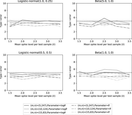
Fig. 9 Power of the two noninferiority tests ($\theta =0.8$) as a function of λ for the different number of microorganisms when detection proportions are fixed at the quantiles of a distribution.

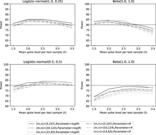
Fig. 10 Power of the two noninferiority tests ($\theta =0.9$) as a function of λ for the different number of microorganisms when detection proportions are fixed at the quantiles of a distribution.

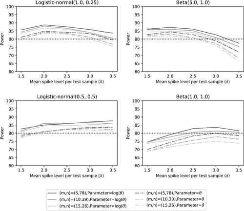
Fig. 11 Power of the two noninferiority tests (θ = 1) as a function of λ for the different number of microorganisms when detection proportions are fixed at the quantiles of a distribution.

For the case of one small detection proportion and four larger detection proportions, we see similar results as for the detection proportions selected at the quantiles. The summary statistics can be found in Table 6, the Type I error can be found in Figure 12, while the power can be found in Figures 13–15.

Fig. 12 Type I error rate of the two noninferiority tests ($\theta =0.7$) as a function of λ for the number of microorganisms m = 5 when detection proportions are fixed with one small value and an average equal to the distribution mean.

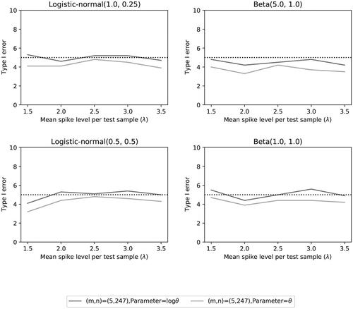
Fig. 13 Power of the two noninferiority tests ($\theta =0.8$) as a function of λ for the number of microorganisms m = 5 when detection proportions are fixed with one small value and an average equal to the distribution mean.

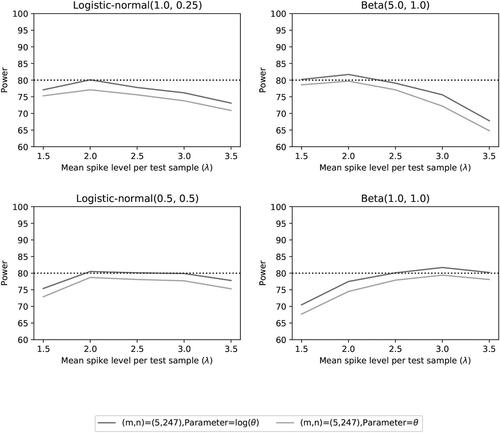
Fig. 14 Power of the two noninferiority tests ($\theta =0.9$) as a function of λ for the number of microorganisms m = 5 when detection proportions are fixed with one small value and an average equal to the distribution mean.

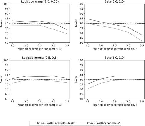
Fig. 15 Power of the two noninferiority tests (θ = 1) as a function of λ for the number of microorganisms m = 5 when detection proportions are fixed with one small value and an average equal to the distribution mean.

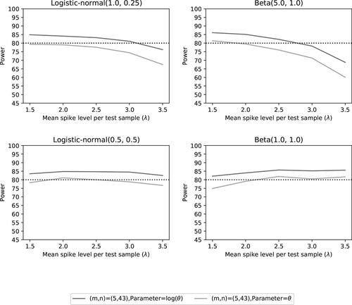
Table 6 Summary statistics of the included number of microorganisms for fixed detection proportions with one small value and an average equal to the distribution mean.

Distribution	$\theta =0.9$				$\theta =1.0$
	Mean	Min	Max	$q_{0.05}$	Mean	Min	Max	$q_{0.05}$
$LN(1,0.25)$	5	5	5	5	4.89	3	5	4
$LN(0.5,0.5)$	5	5	5	5	4.99	4	5	5
B(5,  1)	4.98	4	5	5	4.73	2	5	4
B(1,  1)	5	5	5	5	4.99	4	5	5

Appendix E

PROC NLMIXED DATA = VALIDATION QPOINTS = 20 DF= 10000; PARMS %DO I = 1%TO 16; DET&I = 0.8%END; LOGTHETA=-0.1; %DO I = 1%TO 16; IF MICROORGANISM =&I THEN DO; PC = 1-EXP(-DET&I.*LAMBDA_HAT); PR = 1-EXP(-EXP(LOGTHETA)*DET&I.* LAMBDA_HAT); END; %END; P = (METHOD=’C’)*PC + (METHOD=’R’)*PR; MODEL Y ∼ BINARY(P); ESTIMATE ’LOG ACCURACY’ LOGTHETA ALPHA = 0.1; RUN;

CODE 1. The SAS code for estimating the detection proportions and the common accuracy.

References

- Abbott, W. S. (1925), “A Method of Computing the Effectiveness of an Insecticide,” Journal of Economic Entomology, 18, 265–267. DOI: 10.1093/jee/18.2.265a.
- Cochran, W. G. (1950), “Estimation of Bacterial Densities by Means of the “Most Probable Number”,” Biometrics, 6, 105–116. DOI: 10.2307/3001491.
- Cramér, H. (1946), Mathematical Methods of Statistics, Princeton, NJ: Princeton University Press.
- Donner, A., Birkett, N., and Buck, C. (1981), “Randomization by Cluster: Sample Size Requirements and Analysis,” American Journal of Epidemiology, 114, 906–914. DOI: 10.1093/oxfordjournals.aje.a113261.
- EP 5.1.6. (2017), European Pharmacopoeia 9.2. Alternative Methods for Control of Microbiological Quality, EDQM: Strasbourg, pp. 4339–4348.
- Hahn, G. J., and Meeker, W. Q. (1991), Statistical Intervals: A Guide for Practitioners, New York: Wiley.
- Hsieh, F. Y. (1988), ‘Sample Size Formulae for Intervention Studies With The Cluster as Unit of Randomization,” Statistics in Medicine, 7, 1195–1201. DOI: 10.1002/sim.4780071113.
- IJzerman-Boon, P. C., Manju, M. A., and Van den Heuvel, E. R. (2020), “Non-Inferiority Testing for Qualitative Microbiological Methods: Assessing and Improving the Approach in USP <1223> ,” Manuscript in Preparation.
- IJzerman-Boon, P. C., and Van den Heuvel, E. R. (2015), “Validation of Qualitative Microbiological Test Methods,” Pharmaceutical Statistics, 14, 120–128. DOI: 10.1002/pst.1663.
- Julious, S. A. (2004), ‘Sample Sizes for Clinical Trials With Normal Data,” Statistics in Medicine, 23, 1921–1986. DOI: 10.1002/sim.1783.
- Lu, T. T., and Shiou, S. H. (2002), “Inverses of 2 × 2 Block Matrices,” Computers & Mathematics with Applications, 43, 119–129.
- Manju, M. A., Van den Heuvel, E. R., and IJzerman-Boon, P. C. (2019), “A Comparison of Spiking Experiments to Estimate the Detection Proportion of Qualitative Microbiological Methods,” Journal of Biopharmaceutical Statistics, 29, 30–55. DOI: 10.1080/10543406.2018.1452027.
- Ridout, M. S., Fenlon, J. S., and Hughes, P. R. (1993), “A Generalized One-Hit Model for Bioassays of Insect Viruses,” Biometrics, 49, 1136–1141. DOI: 10.2307/2532255.
- Süli, E. and Mayers, D. F. (2003), An Introduction to Numerical Analysis, Cambridge: Cambridge University Press.
- Sutton, S. V. W., Knapp, J. E., and Dabbah, R. (2001), “Activities of the USP Microbiology Subcommittee of Revision During the 1995–2000 Revision Cycle,” PDA Journal of Pharmaceutical Science and Technology, 55, 33–48.
- USP <1223> (2015), United States Pharmacopoeia 40. Validation of Alternative Microbiological Methods, Rockville, MD: U.S. Pharmacopoeial Convention, pp. 1756–1770.
- Van den Heuvel, E. R. (2011), “Estimation of the Limit of Detection for Quantal Response Bioassays,” Pharmaceutical Statistics, 10, 203–212. DOI: 10.1002/pst.435.
- Van den Heuvel, E. R. and IJzerman-Boon, P. C. (2013), “A Comparison of Test Statistics for the Recovery of Rapid Growth-Based Enumeration Tests,” Pharmaceutical Statistics, 12, 291–299. DOI: 10.1002/pst.1581.
- Wellek, S. (2010), Testing Statistical Hypotheses of Equivalence and Noninferiority, Boca Raton, FL: CRC Press.
- Wyshak, G., and Detre, K. (1972), ‘Estimating the Number of Organisms in Quantal Assays,” Applied Microbiology, 23, 784–790. DOI: 10.1128/am.23.4.784-790.1972.