A Simulation Study on the Estimation of the Effect in the Hypothetical Scenario of No Use of Symptomatic Treatment in Trials for Disease-Modifying Agents for Alzheimer’s Disease

Abstract

In studying a potential disease-modifying treatment for Alzheimer’s Disease, the use of currently available symptomatic medicines—being proportional to the disease progression—can mask the disease-modifying effect. A solution in line with the Estimand framework is to adopt a hypothetical strategy for the intercurrent event “initiation of symptomatic treatment”. However, there is no consensus on reliable estimators for estimands adopting this strategy. To evaluate the performance of several candidate estimators, we have (i) designed clinically realistic data-generating mechanisms based on causal Directed Acyclic Graphs; (ii) selected potentially adequate estimators, amongst other, g-estimation methods usually employed to estimate “controlled direct effect” in mediation analysis; (iii) simulated 10,000 trials for six plausible scenarios and compared the performance of the estimators. The results of our simulations demonstrate that ignoring the intercurrent event introduces a bias compared to the true value of the target estimand. In contrast, g-estimation methods are unbiased, retain nominal power, and control the Type-I error rate at the intended level. Our results can be extrapolated, from a qualitative (absence or presence of bias) but not quantitative point of view (magnitude of the bias), to clinical scenarios with a similar underlying causal structure.

Keywords:

• Causal inference
• Estimands
• g-Estimation
• Hypothetical strategy
• Simulation study

1 Introduction

Alzheimer’s Disease is a neurodegenerative condition, characterized by specific pathological changes in the brain (accumulation of pathological proteins and neuronal death) and clinically by an initial forgetfulness, progressively deteriorating to dementia, with substantial impairment of social functioning and the activities of daily living (Dubois et al. 2010).

The current options for treatment of patients with Alzheimer’s Disease (AD) include treatments that are generally regarded as having a modest effect in improving the symptoms (Lanctôt et al. 2003), affecting neither the underlying pathological process nor the clinical progression of the disease. Conversely, most treatments under investigation are intended as “disease-modifying” treatments, aiming at “impacting the underlying pathology of AD leading to cell death, producing in turn a measurable benefit on the clinical course of AD” (Cummings 2009; Cummings et al. 2019). In particular, such treatments aim at slowing down the progression of the disease.

Developers of disease-modifying treatments are likely to plan clinical trials in a population of patients displaying only initial mild symptoms, in absence of overt dementia (Coric et al. 2015; Ostrowitzki et al. 2017; Egan et al. 2019). On the one hand, this is justified by the clinical objective to prolong a disease status that still allows significant independent personal and social functioning, and a better quality of life (Montgomery et al. 2018; Watt et al. 2019). On the other hand, it also reflects the scientific belief that the pathological process at later stages of the disease becomes more difficult to interrupt (Mehta et al. 2017).

This population, classified as Prodromal Alzheimer’s Disease (Dubois et al. 2014), is unlikely to receive symptomatic medications. However, they are likely to be prescribed one of the available (“symptomatic,” as opposed to “disease-modifying”) treatments upon further progression, at a time subject to significant variability due to variable rates of progression (Komarova and Thalhauser 2011) and different medical practices, even within one region (Purandare et al. 2006).

According to the approach proposed in the Estimand framework (ICH 2019), the initiation of symptomatic medication can be considered an intercurrent event, fulfilling the definition of an “event occurring after treatment initiation that affects either the interpretation or the existence of the measurements associated with the clinical question of interest.” Without accounting for this intercurrent event (IE) in the design or in the analysis of the trials in this setting, the intercurrent event would be (implicitly) handled with the “treatment policy” strategy, and the treatment conditions compared would end up being:

“treatment condition of interest”: Investigational disease-modifying-treatment + symptomatic treatment as per normal clinical practice;

“alternative treatment condition”: Placebo + symptomatic treatment as per normal clinical practice.

In this comparison, the effect measured does not correspond to that of the disease modifying treatment, as it could be confounded by the effect of symptomatic medications. Assuming an efficacious treatment modifying the rate of decline, symptomatic treatment, most often used in patients who are deteriorating the most, would be prescribed with a higher frequency under the alternative treatment condition, leading to a contrast not representative of the full disease modifying effect. The problem is particularly relevant as—for trial efficiency reasons—the population recruited is likely to be enriched with prognostic factors predicting significant decline (in absence of treatment) in the timeframe of the trial (Holland et al. 2012).

Therefore, because trials are by nature of finite duration, the interest could be in studying what would have been happened if the use of symptomatic medications (intercurrent event) would not have occurred, consistent with the “hypothetical” strategy of the Estimand framework.

This is in line with one of the targets of estimation suggested by the EMA Guideline on the clinical investigation of medicines for the treatment of Alzheimer’s disease (EMA 2018). Currently, there is no universally accepted estimator for handling intercurrent events by a hypothetical strategy. Consequently, the aim of this article is to characterize and compare the performance of different candidate estimators for the effect of an investigational disease-modifying treatment for Alzheimer’s Disease in the hypothetical scenario that no patients initiated symptomatic treatment during the study by simulating realistic clinical scenarios. This will include methods that use the observed values after the intercurrent event of interest has occurred (post-IE observations) and methods that discard any post-IE observation. In the following sections we will first describe the data generating mechanisms used in the simulation study. This will be done by first introducing the causal structure of qualitatively different scenarios, and subsequently detailing how the quantitative features of studies were modeled. Next, we will select candidate estimators and performance criteria.

The results will be discussed with the aim of giving practical advice for the analysis of trials in Alzheimer’s Disease and—to the amount that generalization is possible—in other disease areas with a similar underlying causal structure and where a hypothetical strategy is of interest.

2 Methods

2.1 Clinical Question of Interest and Estimand Attributes

The clinical question of interest is whether an investigational medicine slows down progression in subjects with Prodromal AD. There is one intercurrent event, initiation of a symptomatic medication, for which a hypothetical strategy is used. This is reflected in the following Estimand:

“treatment condition of interest”: Investigational disease-modifying treatment without use of symptomatic medications;

“alternative treatment condition”: Placebo without use of symptomatic medications;

“population”: Patients with Prodromal AD;

“Variable”: change in the Clinical Dementia Rating—sum of boxes (CDR-SB) after 24 months as compared to baseline;

“population-level summary”: Difference in mean change in the Clinical Dementia Rating—sum of boxes (CDR-SB) after 24 months.

“Intercurrent event and strategy for handling”: Initiation of symptomatic treatment—hypothetical strategy (as if the IE—i.e., the initiation of symptomatic treatment—had not taken place)

As it will be shown below, this Estimand is the Controlled Direct Effect of the investigational disease-modifying treatment (with no use of symptomatic treatments).

2.2 Data-Generating Mechanism and Simulation Scenarios

The clinical framework is a randomized clinical trial (RCT) where an investigational treatment is compared with placebo in patients with Prodromal Alzheimer’s Disease at 2 years, a common duration for Alzheimer’s trials (Ostrowitzki et al. 2017; Howard et al. 2020), using the CDR-SB (Cedarbaum et al. 2013) as a primary endpoint. CDR-SB covers six cognitive and functional domains with scores ranging from 0 to 18 (higher scores indicate greater impairment).

We consider that the disease-modifying treatment is administered at regular intervals for the whole duration of the trial and that the performance (${\mathrm{Y}}_t)$ is measured at three fixed time points, as defined by the protocol.

The variables we consider are:

$Y_t^{\ast }:$ The value that CDR-SB would have had at time t if patients had not started symptomatic treatment (potentially unobserved);

$Y_t:$ Observed value of CDR-SB at time t. It may differ from $Y_t^{\ast }$ for patients who are taking symptomatic treatment. In our simulation this is only possible at $t = 2$;

$\mathit{prognosis}:$ for each patient, an unobserved patient’s characteristic related to both baseline severity and the decline;

$\mathit{decline}:$ for each patient, an unobserved patient’s characteristic influencing the expected deterioration of symptoms during the trial;

$Z:$ The randomized assignment to placebo or to the investigational disease-modifying treatment (always observed);

$\text{Sym}:$ the status of having started symptomatic treatment (i.e., having encountered the intercurrent event) in consequence of Y₁, assumed to be always observed. $\text{Sym}$ is a mediator of the effect of treatment assignment Z on the outcome $Y_2$, as it lies on the causal pathway from Z to $Y_2$ ($\text{Sym}$ is a node on the directed path Z ->$Y_1$ ->$\text{Sym}$ ->$Y_2)$. The variable $\text{Sym}$ satisfies Last’s definition of a mediator, as “it causes variation in the dependent variable and itself is caused to vary by the independent variable” (Last 2000). In our case, $\text{Sym}$ causes variation in the dependent variable $Y_2$ and is caused to vary (indirectly) by the independent variable Z.

This allows us to apply the findings of mediation research (Pearl 2014) both to better define and to estimate the effect of interest. In line with research on mediation analysis (Pearl 2013), two effects of the treatment on the outcome can be defined, taking “hypothetical” configurations of the mediator. The first is the natural direct effect, comparing outcomes under different treatment conditions while keeping the mediator at the level that would have been observed if all patients were under one of the treatment conditions. In our setting, we would compare a disease modifying treatment and placebo keeping the level of use of symptomatic medication as in the placebo arm in both groups. The controlled direct effect, on the other hand, compares outcomes under different treatment conditions keeping the mediator at an arbitrary fixed level. For this article, the target of estimation is the effect of Z on $Y_2$ in the hypothetical scenario that no patients had had access to symptomatic treatments, a Controlled Direct Effect that can be formalized as follows:(1) $$E[Y_2^{\ast } | Z=1]- E[Y_2^{\ast } | Z=0].$$(1)

In other words, the estimand is the counterfactual difference in outcome between assigning patients to active or placebo, keeping the value of the mediator $\text{Sym}$ fixed at 0.

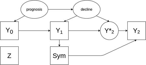
In the following paragraphs, we will describe our simulated scenarios in terms of causal relationships that are included in the simulations. Such relationships will be graphically encoded using directed acyclic graphs (DAGs), (comprehensively described in Pearl 1995 and Elwert 2013). In short, DAGs consist of two elements: variables and arrows. Each variable is represented by a square (if observed) or by an ellipse (if unobserved). Variables are linked by directed arrows indicating a causal relationship, whereby be variable at the beginning of the arrow exerts a direct causal effect on the variable at the end of the arrow. In case no arrow is present, no direct causal effect between two variables exists.

In the subsequent simulation study, we first investigate the null hypothesis (scenario 1)—the causal structure is depicted in the DAG in Figure 1. In this scenario it is assumed that the new treatment is not efficacious (i.e., that patients with $Z=1$ will decline at the same rate as patients with $Z=0)$.

Fig. 1 A directed acyclic graph encoding the causal assumptions regarding the data generating mechanism under the null hypothesis without an effect of the investigational treatment on the outcome (scenario 1). Observed variables are represented as squares, unobserved as ellipses.

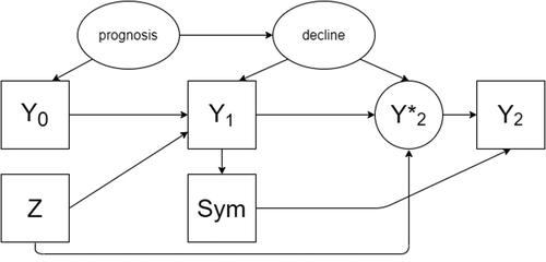
An alternative data-generating mechanism (scenario 2) exists under the hypothesis of presence of treatment effect (Figure 2). In that case, there would also be directed arrows between Z and $Y_1$ and between Z and $Y_2^{\ast }$.

Fig. 2 A directed acyclic graph encoding the causal assumptions regarding the data generating mechanism under the alternative hypothesis with an effect of the treatment on the outcome (scenario 2). Observed variables are represented as squares, unobserved as ellipses.

Overall—compared to most mediation analyses—the case of the hypothetical nonoccurrence of an event in a randomized clinical trial is a privileged situation given that we are allowed by design to consider that the treatment assignment has no causes (hence, no common causes with the intercurrent event).

However, a situation might still occur where the outcome and the intercurrent event have an unmeasured common cause. For example, a patient–physician relationship that is more prone to using symptomatic medication might also be more (or less) proactive in putting in place nonpharmacological measures that might also affect the outcome. Such scenarios (3a, 4b, 4a, and 4b) are described and visualized (Figures S1 and S2) in the supplementary materials.

2.3 Simulation Overview

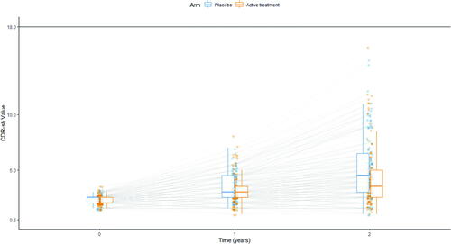
Longitudinal patient-level data on the CDR-SB were simulated based on a nonlinear mixed effects model for a randomized parallel group trial investigating a test drug in comparison to placebo. The total sample size was established at 250 to have an observed power of 90% to detect—under scenario 2—a treatment effect decreasing the decline rate by 25% (the effect simulated in scenarios 2 and 4). The data-generating model is described in detail in the following sections and is illustrated in Figure 3, which shows the longitudinal data of one exemplary trial.

Fig. 3 Illustration of simulated scores. Each line represents the progression of a simulated patient, measured at baseline and after 1 and 2 years. Blue dots are values measured in patients receiving placebo, orange dots values measured in patients receiving the investigational disease modifying treatment. The distribution for each group is described at each of the three timepoints as box-and-whiskers (in blue for patients receiving placebo, in orange for patients receiving the investigational disease-modifying treatment).

2.3.1 Baseline

Clinical trials in the prodromal AD population generally do not use CDR-SB as an inclusion criterion. However, the CDR global score (derived from the same scoring sheet) is generally used, with a required value of 0.5 at baseline. Given the way the CDR global score and the CDR-SB are derived, this implies that CDR-SB baseline severity is at least 0.5. The baseline distribution was simulated in line with the one observed in actual trials (Coric et al. 2015; Ostrowitzki et al. 2017; Egan et al. 2019).

For each patient $i\in \{1,\dots ,\mathrm{n}\}$, the treatment allocation $\text{treat}\in \{1,0\}$ (placebo or active treatment) and baseline prognosis ${\text{prognosis}}_i$ (slow or fast progressor) were simulated as Bernoulli distributed variables with fixed probabilities of 0.5 and 0.1. Subsequently, the baseline severity $Y_{0,i}^{\ast }$, and a natural decline rate were simulated as correlated random intercept and slope from a multivariate normal distribution with a fixed mean for the baseline severity of 2.2. The mean decline rate for each patient depends on the prognosis group, with a mean decline rate of 0.25 for slow and 0.5 for fast progressor. The covariance matrix was set similar to the work of Conrado et al. (2018) to achieve a medium correlation of approximately 0.5 between the baseline CDR-SB and the decline rate, and variances of the baseline score and the decline rate of 0.15 and 0.062, respectively. For both variables, the underlying multivariate distribution was truncated to ensure that the baseline severity was larger or equal than 0.5 and the decline parameter α_i larger than 0.

2.3.2 Disease Progression

The disease course of patients with Alzheimer’s Disease has been studied extensively, in the last few years, in both longitudinal cohorts and control arms of clinical trials. We base the choice of our disease-progression model based on the work of (i) Rogers et al. (Rogers et al. 2012) on combining patient-level and summary data in a meta-analysis for Alzheimer’s disease modeling and simulation and (ii) the Alzheimer’s Disease Neuroimaging Initiative on Disease progression models for the Clinical Dementia Rating–Sum of Boxes (Samtani et al. 2014), which compared a variety of models based on the data of 301 patients with Alzheimer’s disease and mild cognitive impairment patients from the ADNI-1 study who were followed for 2–3 years.

For simulating the longitudinal CDR-SB scores, a beta regression model with Richard’s logistic function as link function was used as the underlying disease progression model.

In short, the value $Y_{t,i}^{\ast }$ for each patient is generated from the beta distribution, which depends on the mean ${\overline{Y}}_{t,i}^{\ast }$. This mean, in turn, is transformed by the link function (in our case, Richard’s function) and modeled based on the natural decline rate and the treatment effect as shown in Equation (6)(6) $$g ({\overline{Y}}_{\tilde{t},i}^{\ast }){=\text{intercept}}_{\tilde{t},\mathrm{ }i}+{\alpha }_i\ast \frac{\tilde{t}-t}{52}\ast {\left(E_{\text{DM}}\right)}^{{\text{treat}}_i}.$$(6) . Here, the disease modifying effect influences the natural decline rate of the respective patient.

More in detail, longitudinal data are simulated for time points t (years) $\in T=\{0, 0.25, 0.5, 0.75, 1, 1.25, 1.5, 1.75, 2\}.$ From these, only data at $t\in \{0, 1, 2\}$ are considered observed and used in the analysis. Following the notation used by Rogers et al., for simulating the underlying CDR-SB scores for each patient i at time t, $Y_{t,i}^{\ast }$, the normalized variable $Y_{t,i}^{\ast }/18$ is simulated using a beta-regression model(2) $$\frac{Y_{t,i}^{\ast }}{18}\sim \text{Beta} \left(\frac{{\overline{Y}}_{t,i}^{\ast }}{18}\ast \tau , \left(1-\frac{{\overline{Y}}_{t,i}^{\ast }}{18}\right)\ast \tau \right)$$(2) where the beta-distribution Beta(a, b) is parameterized with $a= \frac{{\overline{Y}}_{t,i}^{\ast }}{18}\ast \tau$and $b=(1-\frac{{\overline{Y}}_{t,i}^{\ast }}{18})\ast \tau$such that the mean and variance of patient i at time t are(3) $$E\left[\frac{Y_{t,i}^{\ast }}{18}\right]= \frac{{\overline{Y}}_{t,i}^{\ast }}{18}$$(3) (4) $$V\left[\frac{Y_{t,i}^{\ast }}{18}\right]= \frac{\frac{{\overline{Y}}_{t,i}^{\ast }}{18}\ast \left(1-\frac{{\overline{Y}}_{t,i}^{\ast }}{18}\right)}{\tau +1}$$(4) with ${\overline{Y}}_{t,i}^{\ast }$ as the mean of $Y_{t,i}^{\ast }$ and nuisance parameter τ for scaling the variance.

For modeling the conditional expectation for patient i, ${\overline{Y}}_{t,i}^{\ast }$ Richard’s logistic model(5) $$g\left(x\right)=\hspace{0.17em}\text{log}\hspace{0.17em}\left[{\left(\frac{x^{\beta }}{(1-x^{\beta }}\right)}^{1/\beta }\right]$$(5) with $\beta =$3.3 was used as a link function to ensure a sigmoidal shape of the CDR-SB progression and account for the boundedness of the CDR-SB scale at 18 points. For a given time point $t \in T$, the link-transformed expectation of a subsequent time point $\tilde{t}\in T$ with $\tilde{t}>t$ is modeled dependent on the underlying value of the previous time point t and the (baseline) characteristics of the patient as(6) $$g ({\overline{Y}}_{\tilde{t},i}^{\ast }){=\text{intercept}}_{\tilde{t},\mathrm{ }i}+{\alpha }_i\ast \frac{\tilde{t}-t}{52}\ast {\left(E_{\text{DM}}\right)}^{{\text{treat}}_i}.$$(6)

The treatment potentially modifies the natural decline rate with disease modifying treatment effect $E_{\text{DM}}\in (0,1)$, slowing down the decline by a predefined fixed percentage. Particularly, the intercept is calculated from the underlying CDR-SB score of the previous time point, $Y_{t,i}^{\ast },$ by(7) $${\text{intercept}}_{\tilde{t},i}=g\left( Y_{t,i\mathrm{ }}^{\ast }\right)=\hspace{0.17em}\text{log}\hspace{0.17em}\left[{\left( \frac{{\left(\frac{Y_{t,i}^{\ast }}{18}\right)}^{\beta }}{1-{\left(\frac{Y_{t,i}^{\ast }}{18}\right)}^{\beta }}\right)}^{\frac{1}{\beta }}\right] .$$(7)

Samtani et al. found this model to be the best performing disease progression models for which a closed form exists. It is important to note, that the model finally selected by Samtani et al. performed only negligible better regarding Akaike’s Information Criterion, and that Richards model was also used by Conrado et al. in the “Clinical Trial Simulation Tool for Amnestic Mild Cognitive Impairment” for simulating clinical trials in Alzheimer’s Disease with CDR-SB as the primary endpoint. Model nuisance parameter were chosen based on the work of Conrado et al. but slightly modified to fit a typical phase III clinical trial setting (Coric et al. 2015; Ostrowitzki et al. 2017; Egan et al. 2019).

Under the Null hypothesis of no treatment effect, the treatment effect is set to $E_{\text{DM}}=1$ and under the alternative hypothesis, the treatment effect will be set to $E_{\text{DM}}=0.75.$

2.3.3 Intercurrent Event—Start of Symptomatic Treatment

As discussed above, probability of the initiation of symptomatic treatment increases with disease severity and is subject to variability. Estimates of the average effect of symptomatic treatments on the CDR-SB can be derived from clinical trials. Using the mean difference against placebo as the average treatment effect, we have set this parameter to 0.6 (Rogers et al. 1998; Burns et al. 1999).

To calculate the observed CDR-SB values for each patient and time point, the intercurrent event of starting symptomatic treatment needs to be incorporated. At the observed timepoints $T=\{0, 1, 2\}$, the start of symptomatic treatment for each patient was modeled as a Bernoulli random variable ${\text{Sym}}_{t,i}\sim \text{Ber}(p_{t,i})$ with underlying success probability based on a sigmoid function using the underlying CDR-SB score $Y_{t,i\mathrm{ }}^{\ast }$at the given time point:(8) $$p_{t,i}= \frac{1}{1+\hspace{0.17em}\text{exp}\hspace{0.17em}(-\left(Y_{t,i}^{\ast }-5\right))}$$(8) which is truncated at 0 and 1, if needed. In principle, the probability is inversely correlated with the CDR-SB score at the respective time point (i.e., the worse a patient performs, the most likely symptomatic treatment is started). In the presence of a disease-modifying treatment effect, this implies that patients assigned to the treatment group are less likely to start symptomatic treatment as compared to the placebo group. In our simulation, patients stay on symptomatic treatment once they have started. So if ${\text{Sym}}_{t,i\mathrm{ }}=1$ for a given $t\in T$, it follows that ${\text{Sym}}_{\tilde{t},\mathrm{ }i\mathrm{ }}=1$ for all $\tilde{t}\in T$ with $\tilde{t}>t$.

For each patient i, a random effect of the symptomatic treatment $E_{\text{sym},\mathrm{ }i}\sim N{(-0.6, {(0.1)}^2)}_{[-2,0]}$ is simulated from a truncated normal distribution between –2 and 0 with mean –0.6 in line with published magnitudes of symptomatic effects (Rogers et al. 1998; Burns et al. 1999) and standard deviation 0.1. For all time points t, where symptomatic treatment is taken (${\text{Sym}}_{t,i\mathrm{ }}=1)$, this effect is added to the underlying CDR-SB score $Y_{t,i}^{\ast }$ to generate the observed CDR-SB score $Y_{t,i}^{\ast }$, without modifying the decline parameter:(9) $$Y_{t,i}= Y_{t,i}^{\ast }{+\text{Sym}}_{t,i}\ast E_{\text{sym},\mathrm{i}}.$$(9)

The treatment assignment is not used in the calculation of the effect of symptomatic treatment, in line with the assumption that no pharmacological interaction exists between the two. Subsequently, the observed values are truncated at 0 and 18, and both $Y_{t,i}$ and $Y_{t,i}^{\ast }$ are rounded to fit the CDR-SB scale (0, 0.5, 1, 1.5, …, 18). For the comparison of the estimators, only the baseline values, the occurrence of the intercurrent event and the observed CDR-SB values, ${\mathrm{Y}}_{t,i}$, at the modeled time points will be used, whereas the true value of the estimand that employs the hypothetical strategy will be calculated using the underlying values $Y_{t,i}^{\ast }$.

2.3.4 True Value of the Estimand

The true value of the estimand θ is 0 under the Null hypothesis. Under the alternative hypothesis, the true value of the estimand is not a parameter of the data-generating mechanism, as the disease-modifying treatment effect is modeled as a multiplicative effect on the decline in the beta-regression model (see Section 2.2). To derive the true value for each simulation scenario, we estimated the true value based on a trial with 20,000,000 patients for each scenario separately using a linear regression model with treatment and baseline severity as linear predictors and the underlying values of the outcome before applying the effect of the symptomatic medication $Y_2^{\ast }$ as dependent variable.

2.4 Estimators

The estimators tested—in addition to a reference method that will use the unobservable $Y_2^{\ast }$, have been selected to cover a wide range of possible approaches. The selected 13 approaches will include:

• Methods that use post-IE observations (either ignoring the occurrence of the event or de-mediating its effect). Among these, some methods correct in some ways for the effect of the IE, others do not apply further corrections and would generally be considered appropriate for an estimand using the treatment-policy strategy. However, having fixed the choice of Estimand, those are here evaluated as estimators for the Estimand that employs a hypothetical strategy (without the expectation of ideal performance, but for context and comparison);

• Methods that, in line with widespread recommendations (ICH 2018), discard post-IE observations.

All estimators are implemented in R using the referenced functions and packages.

2.4.1 Methods using Post-IE Values

2.4.1.1. Observed values

A linear regression with treatment and baseline severity as linear predictors was performed on the observed values of $Y_2$ (i.e., using the post-IE values). While this estimates the value of an estimand using the treatment policy strategy, it is included here to investigate the magnitude of the bias introduced by ignoring the intercurrent event and to put the result of the other estimators in context.

2.4.1.2. Observed values—adjusted

In addition to the variables included in the prior model, a covariate for starting symptomatic treatment is included in the model.

2.4.1.3. Loh’s g-estimation

Loh and colleagues (Loh et al. 2019) propose a g-estimation method for estimating controlled direct effects in randomized studies, where mediators (like symptomatic treatment start) are present. This allows comparing the potential outcomes under fixed values of the treatment and the mediator (in our case, not-starting symptomatic treatment). Loh’s method was applied to the simulated trials by the following steps:

1. fit a logistic model for the expected value of $\text{Sym}$ using the assigned treatment Z, $Y_0$ and $Y_1$ as predictors with the glm function specifying the “probit” link function;

2. predict the probability to start symptomatic treatment $p_{\text{sym},i}$ by the logistic model for all patients;

3. fit a model for the expected $Y_2$ using as predictors Z, $Y_0$ and $Y_1,\text{Sym}$ and $p_{\text{sym}}$with the lm function;

4. compute a transformed response variable $R_i=Y_{2,i}-\text{coef}(\text{Sym})\ast {\text{Sym}}_i$ using the coefficient of $\text{Sym}$ from step (iii) to remove the effect of the mediator (i.e., the use symptomatic treatment) on the outcome;

5. run a linear regression on the transformed response variable to estimate the direct effect of the treatment with the lm function. The two key assumptions on this method are that (i) no unobserved confounder between treatment and outcome and (ii) no unobserved confounders between the mediator and the outcome exist. While (i) is met in all cases where the treatment is randomized, we designed scenario 4 of our simulation study to violate (ii). To derive estimates for the Standard error, we implemented two approaches: as recommended by Loh et al. (2019), we used bootstrap using the boot function from the R package boot (Davison and Hinkley 1997; Canty and Ripley 2019) with the “basic” method to estimate standard errors, derive confidence intervals and decide about significance. Alternatively, we used the model-derived standard error from step (iv).

2.4.1.4. Linear sequential g-estimation

This method aims at estimating the Controlled Direct Effect through g-estimation (Vansteelandt 2009). The variance estimation is as in Acharya, Blackwell, and Sen (2016). The method was applied using the sequential_g function as implemented in the R package DirectEffects (Matthew Blackwell et al. 2019), specifying $Y_2$ as the outcome, Z and $Y_0$ as baseline variables, $Y_1$ as intermediate variable and $\text{Sym}$as the only variable in the de-mediation function. The sequential g-estimation approach implemented in the sequential_g function in principle follows the same approach as Loh’s sequential g-estimation, but steps (i) and (ii) above are omitted and the predicted probability $p_{\text{sym}}$ is omitted from the de-mediation model in step (iii). Loh and colleagues showed that the estimator for the effect of the mediator derived in step (iii) from Loh’s g-estimation is consistent even if the outcome model in step (iii) is incorrectly specified. In contrast, the estimator for the effect of the mediator on the outcome derived from the sequential g-estimation approach is only consistent if the outcome model is correctly specified (Loh et al. 2019).

2.4.2 Methods not using Post-IE Values

For all methods not using post-IE values, the observed values $Y_2$after the occurrence of the IE were set to missing.

2.4.2.1. Multiple imputation with and without worsening adjustment

Predictive mean matching was implemented in the following steps:

1. Missing data are imputed through predictive mean matching (Rubin 1987) using the mice function implemented in the R package Mice (Buuren and Groothuis-Oudshoorn 2010) using Z, $Y_0$ and $Y_1$ in the prediction matrix for imputation, the mice function imputes missing values by first building a linear regression on all complete cases based on Z, $Y_0$ and $Y_1$ producing regression parameter estimates $\widehat{\beta }$. Second, regression parameters $\tilde{\beta }$ are randomly drawn from the posterior predictive distribution of $\widehat{\beta }$. Third, the outcome for all cases is predicted based on $\tilde{\beta }$ to identify in a fourth step which complete cases are most similar in the predicted values to the predicted value of the missing value. Finally, the observed outcome value for one of the closest five cases is randomly chosen to replace each missing value. The previous steps are repeated to generate five imputed datasets.

2. (only for the methods that apply a worsening adjustment) In line with an Estimator proposed for the estimation of the value of an estimand using the hypothetical strategy for symptomatic medication in Alzheimer’s disease (Polverejan and Dragalin 2020), imputed scores are penalized by 0.5, 2, and 3 (three different estimators tested).

3. Linear regression analyses with Z and $Y_0$ as predictors are performed with the lm function on the five imputed datasets and results are pooled (Rubin 1987) using the pool function from the Mice package.

2.4.2.2. Inverse probability weighting

Inverse probability weighting was carried out in the following steps:

1. a logistic regression model with $1-\text{Sym}$as dependent variable is fitted using $Y_1$ as independent variable with the glm function specifying the “binomial” link function;

2. this model is used to predict probability of not starting $\text{Sym}$;

3. the weights are computed as the inverse of the probability computed above. Extreme weights (top and bottom 2.5%) are trimmed;

4. a weighted linear regression model with Z and $Y_0$ as independent variables on $Y_2$ is performed with the R function glm, using data only from patients that did not start and the above computed weights;

5. Standard errors are computed by bootstrapping using the boot function from the R package boot and the “percent” method to derive standard errors (Davison and Hinkley 1997; Canty and Ripley 2019).

2.4.2.3. Doubly robust inverse probability weighting

Doubly robust estimators combine outcome regression with a model for the probability of completeness of the data (here, the probability of the initiation of symptomatic treatment) to estimate the causal effect of an exposure on an outcome. Doubly robust estimators are unbiased (in large samples) when either the imputation model or the model for the probability of complete data is correctly specified by the user, but not necessarily both (Vansteelandt, Carpenter, and Kenward 2010). The doubly robust estimation was carried out in the following steps (Vansteelandt, Carpenter, and Kenward 2010):

1. A logistic regression model with $1-\text{Sym}$ as dependent variable is fitted using $Y_1$ as independent variable with the glm function specifying the “binomial” link function.

2. This model is used to predict the probability of not starting symptomatic treatment, $P(1-\text{Sym})$.

3. The weights are computed as the inverse of the probability computed above. Extreme weights (top and bottom 2.5%) are trimmed.

4. A weighted regression on $Y_2$ is performed using Z, $Y_0$ and $Y_1$ as independent variables, with the R function glm, using data only from patients that did not start $\text{Sym}$ and the above computed weights.

5. The above regression model is used for predicting $Y_2$ for all patients.

6. A linear regression model with Z and $Y_0$ as independent variables is performed on the predicted outcome variable.

7. Standard errors are computed by bootstrapping using the boot function from the R package boot and the “percent” method to derive standard errors (Davison and Hinkley 1997; Canty and Ripley 2019).

2.4.2.4. Mixed effect model

A mixed model for repeated measures has been fitted using the CDR-SB score at baseline, week 52 and week 104 with treatment, time and the interaction between time and treatment assignment as a fixed effect, using the nlme R package (Pinheiro 2017, #40). Post-IE data are set to missing.

2.5 Performance Criteria

To compare the candidate estimators for the estimand of interest, we primarily investigate the following properties that are averages (or functions of averages) over all simulation runs for the same scenario (Morris, White, and Crowther 2019):

• Bias, expressed in CDR-SB and estimated as $\frac{1}{\mathit{nsim}}\sum {\widehat{\theta }}_k-\theta$ (where nsim is the number of simulations, ${\widehat{\theta }}_k$ is the value of the estimand estimated by each method in a specific simulation run k and $\theta$ is the true value of the estimand in the respective simulation scenario).

• Length of the 95% confidence intervals for ${\widehat{\theta }}_k$, estimated as the mean difference between upper and lower bound of the confidence interval derived with the R function confint based on a normal approximation.

• Coverage, estimated as the % of times θ falls within the confidence interval.

• Square root mean squared error, $\sqrt{\text{MSE}}$, estimated as $\sqrt{\frac{1}{\mathit{nsim}} \sum \widehat{({\theta }_k}-\theta {)}^2 }$on the CDR-SB scale.

• Empirical Type I error/empirical power, measured as the proportion of cases where the null hypothesis was rejected. This will be reported and interpreted as Type I error rate for the scenarios under the null hypothesis (1, 3a, and 3b) and as empirical power in the scenarios where a treatment effect exists (scenarios 2, 4a, and 4b).

For all performance criteria, Monte Carlo estimates of the Standard Errors have been computed (Morris, White, and Crowther 2019).

As a second step, we compare the candidate estimators to the reference estimator using the partly unobserved value $Y_2^{\ast }$that is not affected by starting symptomatic treatment${\theta }_{\mathrm{k}}$. Following this approach, we interpret the reference estimate ${\theta }_{\mathrm{k}}$ as the best estimate that could be derived in the simulation run k for the hypothetical situation that no patients had started symptomatic treatment (as, in fact, $Y_2^{\ast }$is not affected by symptomatic treatment). Subsequently, we calculate the deviation of the estimates from the candidate estimators to the reference estimator as ${\widehat{\theta }}_k-{\theta }_k$. Additionally, we calculate for each simulation run the difference in the number of patients starting symptomatic treatment between treatment groups(10) $${\text{diff}}_{\text{Sym},\text{\hspace{0.05em}k\hspace{0.05em}}}={\sum }_{\mathrm{j}}^{\mathrm{n}}{\text{treat}}_j\ast {\text{Sym}}_{2,j}-({1-\text{treat}}_j)\ast {\text{Sym}}_{2,j} .$$(10)

This will allow us to investigate the performance of the candidate estimators on a simulation run level. In particular, we will investigate the dependency between the deviation from the reference estimator ${\widehat{\theta }}_k-{\theta }_k$ and the difference in patients starting symptomatic treatment between treatment groups ${\text{diff}}_{\text{Sym},\mathrm{k}\mathrm{ }}$.

2.6 Limitations

To allow the investigation of candidate estimators for the estimand of interest handling initiation of symptomatic treatment in AD with a hypothetical strategy, some simplifications and assumptions were necessary.

In our simulation study, we considered only one intercurrent event, while in reality several intercurrent events (and combination thereof) could be of interest (e.g., the co-occurrence of treatment discontinuation). Additionally, for settings in which pharmacological interaction between investigational treatments and additional medications can be reasonably believed to exist, this might have a significant impact on the performance of the estimators proposed, not covered in this article.

The initiation of symptomatic treatment was possible only at one time point in our simulation study. While this represents the causal structure and allows conclusions on classes of estimators, the magnitude of the biases do not directly translate to clinical settings where symptomatic treatment could be started at several time points and the resulting data structure would be slightly more complex.

The problems associated with missing data, which would add another level of complexity the estimation of the treatment effect, have not been included in this simulation study. Follow-up research is needed to assess performance of methods, in case missing data occurs. In particular, the g-estimation methods use the postintercurrent event data, whereas Doubly Robust IPW does not rely on these data. Therefore, if data are missing after the occurrence of the intercurrent event, the performance of g-estimation methods might be impaired more strongly, than the performance of Doubly Robust IPW methods, or methods not using post-intercurrent event data in general.

3 Results

For each of the six scenarios 10,000 trials have been simulated. Below, we first present the results for the null-hypothesis scenario 1 and thereafter the results of the alternative scenario 2. Additional scenarios are reported in the supplementary materials. The summary statistics for the performance criteria are reported in Tables 1, 2, and S2–S5.

Table 1 Performance of estimators under the null hypothesis without unmeasured confounding, scenario 1.

Estimator	Bias (SE${}^{\ast })$	Coverage (SE${}^{\ast })$	sqrMSE (MSE (SE${}^{\ast }))$	CI length (SE${}^{\ast })$	Type I error rate (95% CI${}^{\ast })$
Reference estimator – linear model using $Y_2^{\ast }$	–0.001 (0.003)	95.3 (0.952)	0.269 (0.113 (0.002))	1.329 (0.001)	0.022 (0.019, 0.025)
Observed values${}^{+}$	–0.001 (0.003)	95.18 (0.951)	0.261 (0.106 (0.002))	1.287 (0.001)	0.022 (0.019, 0.025)
Observed values – adjusted${}^{+}$	0 (0.003)	95.14 (0.95)	0.247 (0.095 (0.001))	1.218 (0.001)	0.023 (0.02, 0.026)
Loh’s g-estimation${}^{+}$, model-based SE	–0.001 (0.003)	95.19 (0.951)	0.268 (0.113 (0.002))	1.325 (0.001)	0.022 (0.019, 0.025)
Loh’s g-estimation${}^{+}$, bootstrap based SE	–0.001 (0.003)	95.21 (0.951)	0.268 (0.113 (0.002))	1.322 (0.001)	0.022 (0.019, 0.025)
Linear sequential g-estimation${}^{+}$	–0.001 (0.003)	95.06 (0.949)	0.266 (0.111 (0.002))	1.308 (0.001)	0.023 (0.02, 0.026)
Predictive mean matching (PMM)	0 (0.003)	95.64 (0.955)	0.248 (0.097 (0.001))	1.271 (0.001)	0.02 (0.017, 0.023)
PMM worsening adjustment 0.5	0 (0.003)	95.65 (0.956)	0.256 (0.103 (0.001))	1.308 (0.001)	0.02 (0.017, 0.023)
PMM worsening adjustment 2	0 (0.004)	95.73 (0.956)	0.286 (0.129 (0.002))	1.453 (0.001)	0.02 (0.018, 0.023)
PMM worsening adjustment 3	–0.001 (0.004)	95.66 (0.956)	0.311 (0.152 (0.002))	1.573 (0.001)	0.02 (0.017, 0.023)
Inverse probability weighting	0 (0.005)	93.74 (0.935)	0.397 (0.253 (0.004))	1.882 (0.005)	0.032 (0.029, 0.035)
Doubly robust inverse probability weighting	–0.001 (0.004)	94.77 (0.946)	0.287 (0.129 (0.002))	1.39 (0.001)	0.026 (0.023, 0.029)
Mixed effects model	0 (0.004)	94.75 (0.946)	0.297 (0.139 (0.002))	1.462 (0.001)	0.028 (0.024, 0.031)

Performance parameter are rounded to three digits.

* Monte Carlo estimates of the standard errors.

+ Estimator uses post-IE values.

Table 2 Performance of estimators under Scenario 2, in presence of treatment effect and in absence of confounding between intercurrent event and decline.

Estimator	Bias (SE${}^{\ast })$	Coverage (SE${}^{\ast })$	sqrMSE (MSE (SE${}^{\ast }))$	CI length (SE${}^{\ast }{)}^{\ast }$	Empirical power (95% CI${}^{\ast })$
Reference estimator – linear model using $Y_2^{\ast }$	0.004 (0.003)	94.61 (0.945)	0.235 (0.088 (0.001))	1.167 (0.001)	0.896 (0.89, 0.902)
Observed values${}^{+}$	0.035 (0.003)	94.24 (0.941)	0.229 (0.084 (0.001))	1.13 (0.001)	0.895 (0.889, 0.901)
Observed values – adjusted${}^{+}$	0.122 (0.003)	92.73 (0.924)	0.24 (0.091 (0.001))	1.088 (0.001)	0.855 (0.848, 0.862)
Loh’s g-estimation${}^{+}$, model-based SE	0.007 (0.003)	94.45 (0.943)	0.235 (0.088 (0.001))	1.163 (0.001)	0.897 (0.891, 0.903)
Loh’s g-estimation${}^{+}$, bootstrap based SE	0.007 (0.003)	94.38 (0.942)	0.235 (0.088 (0.001))	1.162 (0.001)	0.893 (0.887, 0.899)
Linear sequential g-estimation${}^{+}$	0.014 (0.003)	94.27 (0.941)	0.233 (0.087 (0.001))	1.148 (0.001)	0.897 (0.891, 0.903)
Predictive mean matching (PMM)	0.152 (0.003)	90.41 (0.899)	0.264 (0.107 (0.001))	1.121 (0.001)	0.8 (0.793, 0.808)
PMM worsening adjustment 0.5	0.127 (0.003)	91.85 (0.915)	0.26 (0.105 (0.001))	1.154 (0.001)	0.805 (0.797, 0.813)
PMM worsening adjustment 2	0.051 (0.003)	94.12 (0.939)	0.266 (0.112 (0.002))	1.288 (0.001)	0.783 (0.775, 0.791)
PMM worsening adjustment 3	0 (0.004)	94.57 (0.944)	0.285 (0.129 (0.002))	1.402 (0.001)	0.756 (0.748, 0.765)
Inverse probability weighting	0.118 (0.004)	91.57 (0.912)	0.332 (0.175 (0.003))	1.532 (0.004)	0.593 (0.583, 0.603)
Doubly robust inverse probability weighting	0.028 (0.003)	94.06 (0.939)	0.252 (0.101 (0.001))	1.217 (0.001)	0.855 (0.848, 0.862)
Mixed effects model	0.107 (0.003)	93.08 (0.928)	0.275 (0.119 (0.002))	1.27 (0.001)	0.746 (0.738, 0.755)

Performance parameter are rounded to three digits.

* Monte Carlo estimates of the standard errors.

+ Estimator uses post-IE values.

3.1 Null-Hypothesis

For the trials simulated under scenario 1, the true value of the estimand of interest was 0. To give clinical context to the results for scenario 1, the average decline in the placebo group was 2.81, the median number of patients starting symptomatic medication was 26.7 (17.8%) in the placebo arm and 26.7 (17.8%) in the active arm. The main results of the simulations are displayed in Tables 1 and Figure 4. It is important to note that none of the investigated methods is biased under the Null hypothesis in scenario 1 and only Inverse Probability Weighting shows a significant increase in the Type I error as the lower limit of the 95%-confidence interval for the one-sided empirical Type I error exceeds 2.5%. This corresponds to a lower coverage for Inverse Probability Weighting as compared to all other candidate estimators.

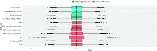
Fig. 4 Distribution of biases for the trials under the null hypothesis (scenario 1). Methods that use post-IE data are plotted in blue and methods that discard post-IE data are plotted in red.

3.2 Alternative Hypothesis

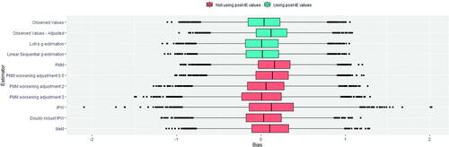
For the trials simulated under scenario 2, the true value of the estimand of interest was –0.95. To give clinical context to the results for scenario 1, the average decline in the placebo group was 2.81 and the median number of patients starting symptomatic medication was 26.7 (17.8%) in the placebo arm and 20.4 (13.6%) in the active arm. The main results of the simulation under scenario 2 are displayed in Tables 2 and Figure 5. For the methods using the post-IE values, the “Observed Value” estimator and the “Observed Value – adjusted” estimator both show an estimated bias of 0.04 and 0.12, respectively. In contrast, the other method using the post-IE values, “Loh’s g-estimation” and “Linear Sequential g-Estimation” show an estimated bias of 0.01 only. As compared to the reference estimator using the true unaffected values, “Observed Value – adjusted” shows a power loss of 4 percentage points, whereas “Observed Value,” “Loh’s g-estimation” and “Linear Sequential g-Estimation” show no power loss. All methods not using the post-IE values show a notable bias in the magnitude of “Observed Value – adjusted” except “doubly robust Inverse Probability Weighting” and “PMM worsening adjustment 3$\prime$.” However, “PMM worsening adjustment 3$\prime$” shows a substantial loss in power of 12 percentage points as compared to the reference estimator. The “Mixed Effects Model” showed a bias of 0.11 and a power loss compared to the reference estimator of 15 percentage points. Overall, the best average performance in terms of bias and power is shown by “Loh’s g-estimation.”

Fig. 5 Distribution of biases for the trials under the alternative hypothesis (scenario 2). Methods that use post-IE data are plotted in blue and methods that discard post-IE data are plotted in red.

An investigation of the dependency of estimators’ performances from the characteristics of each realized trial revealed a significant association, for some of the methods, with the difference in number of patients starting symptomatic medication in each arm.

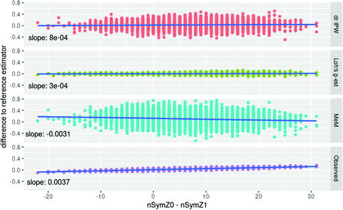
In scenario 2, the average difference in patients starting symptomatic treatment in the two arms is 6.31, with a SD of 6.82. Investigating the dependency of the performance of the estimators on the difference in patients starting symptomatic treatment, we compared the estimators to the reference estimator in those simulation runs, where the difference between patients starting a symptomatic treatment in the placebo arm and those starting it in the active arm exceeds the 90% percentile of 15. In these 914 trials, the mean difference between the candidate estimators and the reference estimator is 0.08 for the “Observed Values” estimator, 0.01 for “Loh’s g-estimation,” 0.07 for the “Mixed Effects Model,” and 0.03 for the “doubly robust Inverse Probability Weighting.”

Such dependency for the “Observed Values” estimator is also present under the null hypothesis. In scenario 1, the average difference in patients starting symptomatic treatment in the two arms is 0, with a SD of 7.21. Investigating the dependency of the performance of the estimators on the difference in patients starting symptomatic treatment, we compared the estimators to the reference estimator in those simulation runs, where the difference between patients starting a symptomatic treatment in the placebo arm and those starting it in the active arm exceeds the 90% percentile of 9. In these 956 trials, the mean difference between the candidate estimators to the reference estimator is 0.04 for the “Observed Values” estimator, 0.002 for “Loh’s g-estimation,” –0.06 for the “Mixed Effects Model,” and 0.01 for the “doubly robust Inverse Probability Weighting” (Figure 6).

Fig. 6 Dependency between the performance and the difference in starting symptomatic treatment between treatment groups in scenario 2. The difference between the candidate estimator and the reference estimator depends on the difference in starting symptomatic treatment between treatment groups for the Mixed effects Model (MeM) setting values after initiation of symptomatic treatment to missing, and using the observed values in a linear model (Observed). No such dependency is observed for Doubly Robust IPW (drIPW) and Loh’s g-estimation (Loh’s g-est).

4 Discussion

In this article, we compared several candidate estimators for the effect of an investigational disease-modifying treatment for Alzheimer’s disease in the hypothetical scenario that no patients initiated symptomatic treatment during the study. Using a realistic data-generating model, we investigated the performance in different clinical scenarios, both under the null- and alternative hypothesis, and in the presence and absence of unmeasured confounding.

In absence of a treatment effect, all estimators are unbiased. This is in line with expectations, since no open backdoor path—a noncausal indirect connection between the variables (Cunningham 2021)—exists from Z to $Y_2$ in Figure 1 and S1 (that is, no path at all exists). Furthermore, most investigated estimators control the Type-I error given the data generating mechanisms used. However, a small Type-I error rate increase is observed for IPW in all scenarios under the null hypothesis and for Doubly Robust IPW under the presence of unmeasured confounding. In accordance, in these scenarios, the coverage of IPW and Doubly Robust IPW is below the nominal level of 95%. While on average the Observed Values estimator is not biased, it can deviate from the reference estimator (in both directions) in some realizations. Similarly, the Mixed effects model is not biased under the null hypothesis but are less precise than g-estimation methods.

Using the Observed Values showed a systematic bias under the alternative hypothesis. This was to be expected given that next to the treatment effect of interest (the direct effect of Z on $Y_2$ and the effect of Z on $Y_2$ mediated through) the path $Z\to Y_1\to \text{Sym}\to Y_2$ is open. We observe that this bias was—on average—not of a clinically relevant size. This is in line with the prediction formulated by Donohue and colleagues following a different approach (Donohue et al. 2020). However, while the presence of bias can be generalized, its magnitude cannot. In our results there is a positive correlation between (i) the difference in the estimates using “Observed Values” method and the reference estimator and (ii) the difference in proportions starting symptomatic treatment between the treatment groups. While in most (but not all) of the simulated trials the proportions of patients starting symptomatic treatment were similar enough not to introduce substantial differences, and the average difference between proportions was not large, this depends on the data generating model and could be substantially different in a real clinical trial setting. An imbalance in the proportions of patients starting symptomatic treatment in the two arms is more likely in trials with a stronger effect of the investigational treatment and a more homogeneous prescribing threshold for the symptomatic treatment across the study centers. Importantly, it will be difficult to know a priori whether small or large imbalances can be expected in any specific trial. Even under the null hypothesis—while the method is on average unbiased and very substantial imbalances are unlikely—they could still occur—in any direction—by chance. In summary, although the average performance of using only Observed Values was only slightly biased, this method cannot be recommended. If used, the imbalance in starting symptomatic treatment needs to be investigated post hoc.

Additionally, the comparison between the linear regression model with treatment and baseline severity as independent variables using either the observed value or the true underlying value not affected by symptomatic treatment (the reference model) highlights two aspects: first, using the observed values leads to a small bias underestimating the treatment effect. Second, the confidence interval length (and therefore the estimated standard error) is downward biased when the observed values are used as compared to using the underlying unaffected values. In our simulations, these effects—the underestimation of the treatment effect and the underestimation of the standard error—canceled each other out, resulting in a comparable power for the reference method and the linear model based on the observed values. Depending on the clinical scenario (or simulation parameters) this does not always need to be the case. The principle limitations of using the observed values as dependent variable in a linear model adjusted for baseline severity cannot be overcome by additionally adjusting for starting symptomatic treatment by a linear predictor. By stratifying the analysis for$\text{Sym}$, we condition on a descendant of the collider $Y_1$ on the formerly closed path $Z\to Y_{1\mathrm{ }}\leftarrow \text{decline}\to Y_2,$and thus open this backdoor path from Z to $Y_2$. This is reflected in bias and coverage below the nominal level.

An estimator that is more robust and showed the best performance are the g-estimation approaches, especially as proposed by Loh and colleagues (Loh et al. 2019). By de-mediating the effect of starting symptomatic treatment, these methods isolate the direct effect of the disease modifying treatment, and thus compensate for a differential start of symptomatic treatment. Also in the additional scenarios introducing an unmeasured confounder (see supplementary materials) no relevant bias was introduced, and the Type-I error rate was controlled. Additionally, the originally intended power was provided by Loh’s g-estimation approach whereas most other methods suffer from a power loss as compared to the reference method. In our simulation scenarios, there was no qualitative difference between using the model-based standard error estimates and using a bootstrap approach to derive standard errors as proposed by Loh et al. (2019).

The performance was overall worse for estimators that—in line with recommendations issued by the International Council for Harmonization (ICH) and recently published elsewhere (ICH 2018; Mallinckrodt et al. 2019)—discarded post-IE observations and applied the normal techniques for missing data problems. Mixed Effects Models are often employed for the analysis of clinical trials in Alzheimer’s disease (Ostrowitzki et al. 2017; Boada et al. 2020; FDA 2020) and discarding post-IE data is the most widespread approach in estimating a hypothetical effect. Therefore, Mixed Effect Models estimator with post-IE dataset to missing is a de facto standard. However, in our simulations Mixed Effects Model demonstrated a reduction of power and biased effect estimates under the alternative hypothesis. In scenario 2, the power for the Mixed Effects Model setting post-IE values to missing was below 75% whereas the g-estimation methods retained the nominal power of 90%. Such results can be explained with the violation of the linearity assumptions made in the mixed model when implicitly imputing $Y_2$ for patients starting symptomatic treatment based on the estimated covariance structure. In the data generation model, however, the increase in $Y_2$ follows a sigmoid shape with a larger slope for patients with a medium score. This problem is increased by the fact that patients with a high value for $Y_1$ are starting symptomatic treatment with a high probability, they are likely underrepresented or absent in the dataset for estimating the model parameters and thus, the decline might be underestimated. This mechanism is illustrated in Figures S3–S5 in the supplementary materials. Figure S3 shows that linearity does not hold for the progression, and Figures S4 and S5 illustrate that patients with high values for $Y_2$are systematically missing in the analysis dataset used in the mixed model. This problem is related to “donor sparseness” as discussed by Morris, White, and Royston (2014), which could occur if the imputed data are not Missing Completely At Random (which is the case in our DGM). With a higher proportion of patients starting symptomatic treatment in the placebo group under the alternative hypothesis, this leads to an underestimation of the treatment effect.

Doubly Robust IPW does not systematically introduce bias, this is in line with the assumptions of exchangeability, consistency and (at least structurally) positivity (Hernán and Robins 2020) being met in our simulations. However, the larger confidence interval length observed with Doubly Robust IPW points to bigger imprecision as compared to g-estimation methods. This method also provided a smaller power as compared to g-estimation methods. It should be observed that—while the positivity assumption ($P(\text{Sym}=0|Z=z, Y=y, Y_1=y_1)>0)$is met in principle, there might be in some realizations—on a probabilistic basis—a threshold $a>0$, so that (i) there are patients with $Y_1>a$ and (ii) all patients with $Y_1>a$ start symptomatic treatment. Consequently, the conditional probability for not starting $\text{Sym}$ is 0 for a subset of patients with $P(Y_1>a)>0$. This “random violation” of the positivity assumption could lead to biased estimates. This problem has also been highlighted Mallinckrodt et al. (2019), but the magnitude of potential bias cannot be anticipated.

Inverse Probability Weighting and multiple imputation via Predictive Mean Matching showed biases, underestimated the disease-modifying treatment effect and did not retain the intended power. The underestimation of the treatment effect by the Predictive Mean Matching could be explained as follows. Constructing the five nearest neighbors to a patient, who starts symptomatic treatment, based on predicted means does not ensure that the mean of these five nearest neighbors equals the true value in expectation. Potentially, the mean of the five neighbors underestimates the true mean, which would lead to an underestimation of the decline in patients starting symptomatic treatment (most represented in the placebo group). This problem has been pointed out by Morris et al. (2014) as “donor sparseness,” as discussed above in the context of mixed models. In the supplementary materiald, Figure S3 illustrates the bias introduced by donor sparseness in the context of predictive mean matching. In line with this, the worsening adjustment of the imputed scores as suggested by Polverejan and colleagues improves the performance of the multiple imputation method tested. A critical limitation of this approach is the dependency of the performance upon the value used for correction. Further research might propose ways to derive such value from the data. Until then, this method cannot be recommended.

Our results can be generalized qualitatively: the presence or absence of systematic biases for the different methods can be generalized to problems with a similar causal structure. On the other hand, the quantitative elements (both magnitude and direction of biases) are specific to the setting we have simulated. In particular, the magnitude of the effect of the symptomatic treatment is known to be much smaller in Alzheimer’s Disease than in other conditions (e.g., in Parkinson’s Disease). It is likely that the methods that introduce a systematic bias in our simulations would introduce a bias of greater magnitude in other conditions. Similarly, more complex data generating mechanisms (e.g., including a pharmacodynamic interaction between the disease-modifying and the symptomatic treatment) have not been simulated here and might deserve different considerations.

The satisfactory characteristics of the sequential g-estimation methods are supported by previous research (Goetgeluk, Vansteelandt, and Goetghebeur 2008; Lepage et al. 2016; Valente, MacKinnon, and Mazza 2020) in problems with an analogous causal structure. These suggest that de-mediating approaches are a meaningful alternative to imputation-based approaches. Our results also have implications for trial conduct, and for data collection in particular: the implementation of both the “Observed Values” and the g-estimation estimators (including in Loh’s implementation) require that data are collected even following the occurrence of the intercurrent event for which a hypothetical strategy is adopted.

At the best of our knowledge at the time of writing, this is the first simulation study applying such methods in the context of the ICH E9 R1 Estimands’ framework and including a comparison with multiple imputation methods.

In summary, our simulation study showed that under the assumed causal structure g-estimation methods, especially as proposed by Loh and colleagues are promising candidates for estimating a disease-modifying treatment effect in the hypothetical scenario that no patients initiated symptomatic treatment during the study.

Supplementary Materials

Supplementary Material contain details on additional scenarios (with an unmeasured confounder between decline and the IE) and an illustration of a reason why methods setting data at missing might be biased.

Disclosure Statement

The authors have no conflicts of interest to declare. The views expressed in this article are the personal views of the authors and may not be understood or quoted as being made on behalf of or reflecting the position of the agencies or organizations with which the authors are affiliated.

Funding

The author(s) reported there is no funding associated with the work featured in this article.

References

- Acharya, A., Blackwell, M., and Sen, M. (2016), “Explaining Causal Findings Without Bias: Detecting and Assessing Direct Effects,” American Political Science Review, 110, 512–529. DOI: 10.1017/S0003055416000216.
- Boada, M., López, O. L., Olazarán, J., Núñez, L., Pfeffer, M., Paricio, M., Lorites, J., Piñol-Ripoll, G., Gámez, J. E., and Anaya, F. (2020), “A Randomized, Controlled Clinical Trial of Plasma Exchange with Albumin Replacement for Alzheimer’s Disease: Primary Results of the AMBAR Study,” Alzheimer’s & Dementia, 16, 1412–1425.
- Burns, A., Rossor, M., Hecker, J., Gauthier, S., Petit, H., Möller, H.-J., Rogers, S., and Friedhoff, L. (1999), “The Effects of Donepezil in Alzheimer’s Disease—Results from a Multinational Trial 1,” Dementia and Geriatric Cognitive Disorders, 10, 237–244. DOI: 10.1159/000017126.
- Buuren, S. V., and Groothuis-Oudshoorn, K. (2010), “mice: Multivariate Imputation by Chained Equations in R,” Journal of Statistical Software, 45, 1–68.
- Canty, A., and Ripley, B. (2019), “boot: Bootstrap R (S-Plus) Functions,” R Package Version 1. 3–22, 1.
- Cedarbaum, J. M., Jaros, M., Hernandez, C., Coley, N., Andrieu, S., Grundman, M., Vellas, B., and Alzheimer’s Disease Neuroimaging Initiative. (2013), “Rationale for use of the Clinical Dementia Rating Sum of Boxes as a primary outcome measure for Alzheimer’s disease clinical trials,” Alzheimer’s & Dementia, 9, S45–S55.
- Conrado, D. J., Willis, B., Sinha, V., Nicholas, T., Burton, J., Stone, J., Chen, D., Coello, N., Wang, W., and Kern, V. D. (2018), “Towards FDA and EMA Endorsement* of a Clinical Trial Simulation Tool for Amnestic Mild Cognitive Impairment,” Journal of Pharmacokinetics and Pharmacodynamics, 45, S17.
- Coric, V., Salloway, S., van Dyck, C. H., Dubois, B., Andreasen, N., Brody, M., Curtis, C., Soininen, H., Thein, S., and Shiovitz, T. (2015), “Targeting Prodromal Alzheimer Disease with Avagacestat: A Randomized Clinical Trial,” JAMA Neurology, 72, 1324–1333. DOI: 10.1001/jamaneurol.2015.0607.
- Cummings, J., Lee, G., Ritter, A., Sabbagh, M., and Zhong, K. (2019), “Alzheimer’s Disease Drug Development Pipeline: 2019,” Alzheimer’s & Dementia: Translational Research & Clinical Intervention, 5, 272–293. DOI: 10.1016/j.trci.2019.05.008.
- Cummings, J. L. (2009), “Defining and Labeling Disease-Modifying Treatments for Alzheimer’s Disease,” Alzheimer’s & Dementia, 5, 406–418.
- Cunningham, S. (2021), Causal Inference, New Haven, CT: Yale University Press.
- Davison, A. C., and Hinkley, D. V. (1997), Bootstrap Methods and Their Application, New York: Cambridge University Press.
- Donohue, M. C., Model, F., Delmar, P., Volye, N., Liu-Seifert, H., Rafii, M. S., Aisen, P. S., and Alzheimer’s Disease Neuroimaging Initiative (2020), “Initiation of Symptomatic Medication in Alzheimer’s Disease Clinical Trials: Hypothetical Versus Treatment Policy Approach,” Alzheimer’s & Dementia, 16, 797–803. DOI: 10.1002/alz.12058.
- Dubois, B., Feldman, H. H., Jacova, C., Cummings, J. L., Dekosky, S. T., Barberger-Gateau, P., Delacourte, A., Frisoni, G., Fox, N. C., and Galasko, D. (2010), “Revising the Definition of Alzheimer’s Disease: A New Lexicon,” The Lancet Neurology, 9, 1118–1127. DOI: 10.1016/S1474-4422(10)70223-4.
- Dubois, B., Feldman, H. H., Jacova, C., Hampel, H., Molinuevo, J. L., Blennow, K., DeKosky, S. T., Gauthier, S., Selkoe, D., and Bateman, R. (2014), “Advancing Research Diagnostic Criteria for Alzheimer’s Disease: The IWG-2 Criteria,” The Lancet Neurology, 13, 614–629. DOI: 10.1016/S1474-4422(14)70090-0.
- Egan, M. F., Kost, J., Voss, T., Mukai, Y., Aisen, P. S., Cummings, J. L., Tariot, P. N., Vellas, B., van Dyck, C. H., and Boada, M. (2019), “Randomized Trial of Verubecestat for Prodromal Alzheimer’s Disease,” The New England Journal of Medicine, 380, 1408–1420. DOI: 10.1056/NEJMoa1812840.
- Elwert, F. (2013), “Graphical Causal Models,” in Handbook of Causal Analysis for Social Research, eds. S. L. Morgan, pp. 245–273, Dordrecht: Springer.
- EMA (2018), “Guideline on the Clinical Investigation of Medicines for the Treatment of Alzheimer’s Disease.”
- FDA (2020), “Combined FDA and Applicant PCNS Drugs Advisory Committee Briefing Document,” available at https://www.fda.gov/media/143502/download.
- Goetgeluk, S., Vansteelandt, S., and Goetghebeur, E. (2008), “Estimation of Controlled Direct Effects,” Journal of the Royal Statistical Society, Series B, 70, 1049–1066. DOI: 10.1111/j.1467-9868.2008.00673.x.
- Hernán, M. A., and Robins, J. M. (2020), Causal Inference: What If, Boca Raton, FL: Chapman & Hill/CRC.
- Holland, D., McEvoy, L. K., Desikan, R. S., Dale, A. M., and Alzheimer’s Disease Neuroimaging Initiative. (2012), “Enrichment and Stratification for Predementia Alzheimer Disease Clinical Trials,” PloS One, 7, e47739. DOI: 10.1371/journal.pone.0047739.
- Howard, R., Zubko, O., Bradley, R., Harper, E., Pank, L., O’Brien, J., Fox, C., Tabet, N., Livingston, G., and Bentham, P. (2020), “Minocycline at 2 Ddifferent Dosages vs Placebo for Patients with Mild Alzheimer Disease: A Randomized Clinical Trial,” JAMA Neurology, 77, 164–174. DOI: 10.1001/jamaneurol.2019.3762.
- ICH (2018), “ICH E9(R1) Step 2 Training Material.” odule 2.3—Estimands.
- ICH (2019), “Addendum on Estimands and Sensitivity Analysis in Clinical Trials to the Guideline on Statistical Principles for Clinical Trials E9(R1).”
- Komarova, N. L., and Thalhauser, C. J. (2011), “High Degree of Heterogeneity in Alzheimer’s Disease Progression Patterns,” PLoS Computational Biology, 7, e1002251. DOI: 10.1371/journal.pcbi.1002251.
- Lanctôt, K. L., Herrmann, N., Yau, K. K., Khan, L. R., Liu, B. A., LouLou, M. M., and Einarson, T. R. (2003), “Efficacy and Safety of Cholinesterase Inhibitors in Alzheimer’s Disease: A Meta-Analysis,” CMAJ, 169, 557–564.
- Last, J. (2000), A Dictionary of Epidemiology (4th ed.), New York: Oxford University Press.
- Lepage, B., Dedieu, D., Savy, N., and Lang, T. (2016), “Estimating Controlled Direct Effects in the Presence of Intermediate Confounding of the Mediator-Outcome Relationship: Comparison of Five Different Methods,” Statistical Methods in Medical Research, 25, 553–570. DOI: 10.1177/0962280212461194.
- Loh, W. W., Moerkerke, B., Loeys, T., Poppe, L., Crombez, G., and Vansteelandt, S. (2019), “Estimation of Controlled Direct Effects in Longitudinal Mediation Analyses with Latent Variables in Randomized Studies,” Multivariate Behavioral Research, 55, 763–785. DOI: 10.1080/00273171.2019.1681251.
- Mallinckrodt, C., Molenberghs, G., Lipkovich, I., and Ratitch, B. (2019), Estimands, Estimators and Sensitivity Analysis in Clinical Trials, Boca Raton, FL: CRC Press.
- Matthew Blackwell, A. A., Sen, M., Kuriwaki, S., and Brown, J. (2019), “DirectEffects: Estimating Controlled Direct Effects for Explaining,” available at https://cran.r-project.org/web/packages/DirectEffects/index.html
- Mehta, D., Jackson, R., Paul, G., Shi, J., and Sabbagh, M. (2017), “Why do Trials for Alzheimer’s Disease Drugs Keep Failing? A Discontinued Drug Perspective for 2010–2015,” Expert Opinion on Investigational Drugs, 26, 735–739. DOI: 10.1080/13543784.2017.1323868.
- Montgomery, W., Goren, A., Kahle-Wrobleski, K., Nakamura, T., and Ueda, K. (2018), “Alzheimer’s Disease Severity and its Association with Patient and Caregiver Quality of Life in Japan: Results of a Community-Based Survey,” BMC Geriatrics, 18, 141. DOI: 10.1186/s12877-018-0831-2.
- Morris, T. P., White, I. R., and Crowther, M. J. (2019), “Using Simulation Studies to Evaluate Statistical Methods,” Statistics in Medicine, 38, 2074–2102. DOI: 10.1002/sim.8086.
- Morris, T. P., White, I. R., and Royston, P. (2014), “Tuning Multiple Imputation by Predictive Mean Matching and Local Residual Draws,” BMC Medical Research Methodology, 14, 1–13. DOI: 10.1186/1471-2288-14-75.
- Ostrowitzki, S., Lasser, R. A., Dorflinger, E., Scheltens, P., Barkhof, F., Nikolcheva, T., Ashford, E., Retout, S., Hofmann, C., Delmar. (2017), “A Phase III Randomized Trial of Gantenerumab in Prodromal Alzheimer’s Disease,” Alzheimer’s Research & Therapy, 9, 95.
- Pearl, J. (1995), “Causal Diagrams for Empirical Research,” Biometrika, 82, 669–688. DOI: 10.1093/biomet/82.4.669.
- Pearl, J. (2013), “Direct and Indirect Effects,” arXiv Preprint arXiv:1301.2300
- Pearl, J. (2014), “Interpretation and Identification of Causal Mediation,” Psychological Methods, 19, 459–481.
- Polverejan, E., and Dragalin, V. (2020), “Aligning Treatment Policy Estimands and Estimators—A Simulation Study in Alzheimer’s Disease,” Statistics in Biopharmaceutical Research, 12, 142–154. DOI: 10.1080/19466315.2019.1689845.
- Purandare, N., Swarbrick, C., Fischer, A., and Burns, A. (2006), “Cholinesterase Inhibitors for Alzheimer’s Disease: Variations in Clinical Practice in the North–West of England,” International Journal of Geriatric Psychiatry, 21, 961–964. DOI: 10.1002/gps.1591.
- Rogers, J. A., Polhamus, D., Gillespie, W. R., Ito, K., Romero, K., Qiu, R., Stephenson, D., Gastonguay, M. R., and Corrigan, B. (2012), “Combining Patient-Level and Summary-Level Data for Alzheimer’s Disease Modeling and Simulation: A β Regression Meta-Analysis,” Journal of Pharmacokinetics and Pharmacodynamics, 39, 479–498. DOI: 10.1007/s10928-012-9263-3.
- Rogers, S., Farlow, M., Doody, R., Mohs, R., and Friedhoff, L. (1998), “A 24-Week, Double-Blind, Placebo-Controlled Trial of Donepezil in Patients with Alzheimer’s Disease. Donepezil Study Group,” Neurology, 50, 136–145. DOI: 10.1212/wnl.50.1.136.
- Rubin, D. B. (1987), Multiple Imputation for Nonresponse in Surveys, New York: Wiley.
- Samtani, M. N., Raghavan, N., Novak, G., Nandy, P., and Narayan, V. A. (2014), “Disease Progression Model for Clinical Dementia Rating-Sum of Boxes in Mild Cognitive Impairment and Alzheimer’s Subjects from the Alzheimer’s Disease Neuroimaging Initiative,” Neuropsychiatric Disease and Treatment, 10, 929–952. DOI: 10.2147/NDT.S62323.
- Valente, M. J., MacKinnon, D. P., and Mazza, G. L. (2020), “A Viable Alternative When Propensity Scores Fail: Evaluation of Inverse Propensity Weighting and Sequential G-Estimation in a Two-Wave Mediation Model,” Multivariate Behavioral Research, 55, 165–187. DOI: 10.1080/00273171.2019.1614429.
- Vansteelandt, S. (2009), “Estimating Direct Effects in Cohort and Case–Control Studies,” Epidemiology (Cambridge, Mass.), 20, 851–860. DOI: 10.1097/EDE.0b013e3181b6f4c9.
- Vansteelandt, S., Carpenter, J., and Kenward, M. G. (2010), “Analysis of Incomplete Data using Inverse Probability Weighting and Doubly Robust Estimators,” Methodology, 6, 37–48. DOI: 10.1027/1614-2241/a000005.
- Watt, A. D., Jenkins, N. L., McColl, G., Collins, S., and Desmond, P. M. (2019), “Ethical Issues in the Treatment of Late-Stage Alzheimer’s Disease,” Journal of Alzheimer’s Disease, 68, 1311–1316. DOI: 10.3233/JAD-180865.