An Alternative to Traditional Sample Size Determination for Small Patient Populations

Abstract

The majority of phase III clinical trials use a 2-arm randomized controlled trial with 50% allocation between the control treatment and experimental treatment. The sample size calculated for these clinical trials normally guarantee a power of at least 80% for a certain Type I error, usually 5%. However, these sample size calculations, do not typically take into account the total patient population that may benefit from the treatment investigated. In this article, we discuss two methods, which optimize the sample size of phase III clinical trial designs, to maximize the benefit to patients for the total patient population. We do this for trials that use a continuous endpoint, when the total patient population is small (i.e., for rare diseases). One approach uses a point estimate for the treatment effect to optimize the sample size and the second uses a distribution on the treatment effect in order to account for the uncertainty in the estimated treatment effect. Both one-stage and two-stage clinical trials, using three different stopping boundaries are investigated and compared, using efficacy and ethical measures. A completed clinical trial in patients with anti-neutrophil cytoplasmic antibody (ANCA)-associated vasculitis is used to demonstrate the use of the method. Supplementary materials for this article are available online.

Keywords:

• Continuous response
• Patient benefit
• Rare disease
• Sequential design

1 Introduction

The design most often used in Phase III superiority clinical trials is a two-arm randomized controlled trial (RCT) with equal allocation between treatment arms (Sibbald and Roland 1998). This method assigns each patient to the experimental treatment or the control treatment (placebo or standard of care) with a fixed probability of 50%. At the end of said superiority trial the outcomes of the two treatments are compared using a one-sided two sample hypothesis test, with a pre-specified Type I error, α, (usually $\alpha =5\%$). If the p-value calculated from the test is smaller than α then the null hypothesis of “the experimental treatment is not superior to the control treatment” is rejected, (see Lieberman 2001). Then, the experimental treatment will either under go further testing, or an application to a regulatory agency (e.g., the FDA) will be made, so that the treatment can be given to future patients, (see Tonkens 2005). If the p-value is larger than or equal to α the null hypothesis cannot be rejected and therefore, the testing on the experimental drug is likely to stop and the standard of care treatment will carry on being given to patients.

If the primary outcome of the RCT is normally distributed, $Y_k\sim N({\mu }_k,{\sigma }^2)$ for both the control treatment, k = C and the experimental treatment, k = E, then the equation below,(1) $$n=\frac{4·{\sigma }^2{({\Phi }^{-1}(1-\alpha )+{\Phi }^{-1}(1-\beta ))}^2}{{\delta }^2},$$(1) can be used to determine the sample size, n, of the RCT. The sample size calculated using Equation (1)(1) $$n=\frac{4·{\sigma }^2{({\Phi }^{-1}(1-\alpha )+{\Phi }^{-1}(1-\beta ))}^2}{{\delta }^2},$$(1) will ensure a trial with power ($1-\beta$), if a difference in treatment means ($\delta ={\mu }_E-{\mu }_C$) and common standard deviation (σ) is present, for a specified Type I error (α) (Charan and Biswas 2013). This sample size determination does not take into account the total patient population, that is all patients that could potentially benefit from the treatment.

For some rare diseases, Equation (1)(1) $$n=\frac{4·{\sigma }^2{({\Phi }^{-1}(1-\alpha )+{\Phi }^{-1}(1-\beta ))}^2}{{\delta }^2},$$(1) may produce a trial size which is a large proportion of the total patient population. For example, for a Type I error, α, of 5%, a Type II error, β, of 20%, a standard deviation, σ, of 1.5 and a difference in treatment means, δ of 0.4, results in a sample size of 348. The anti-neutrophil cytoplasmic antibody (ANCA)-associated vasculitis (AAV) are rare multisystem autoimmune diseases, thought to have a prevalence of 46–184 per million (Yates and Watts 2017). If we assume a prevalence of 100 per million, this would give a patient population of roughly 6680 in the United Kingdom. Hence, in a rare disease trial where the total patient population might only be N = 6680, a trial size of n = 348 would result in a high proportion (5.2%) of patients in the trial.

There are a number of reasons why having a large proportion of the patient population in the clinical trial is not desirable. First, there will only be a relatively small proportion of patients outside the trial, who will actually benefit from the results of the trial. Furthermore, the larger the trial, the more patients are allocated to the lesser treatment (Faber and Fonseca 2014), due to half the trial population receiving the inferior treatment by design.

These issues highlight the difficulty associated with determining the sample size for a clinical trial, particularly in a small population. It must be large enough to provide a reliable decision on which treatment is superior. However, it should not be too large, so that extra patients are being given a noneffective drug unnecessarily. In small patient populations this difficulty only increases.

The effect of the total patient population, N, on the sample size of a trial, n, has been explored by Stallard et al. (2017). They look to maximize a gain function that captures any kind of cost, loss or benefit associated with the treatment, using a decision theoretical approach. Furthermore, Colton (1963) investigates a minimax procedure to minimize an expected loss function and a maximin procedure to maximize an expected net gain function, where each of these functions is proportional to the true difference in treatment means, δ, and incorporates the total patient population, N. Additionally, Cheng, Su, and Berry (2003) explores a decision-analytic approach to determine a trial’s sample size. They assume the total patient horizon is treated in a fixed number of stages and they choose the size of each stage in order to maximize the number of patient successes. This article focuses on binary patient outcomes, when the success probability of one arm is known and when the success probabilities of both arms are unknown.

Similarly to Kaptein (2019), we aim to optimize the sample size of a phase III superiority clinical trial in order to maximize the patient benefit for the whole patient population, N, and we assume that N is finite and fixed. Kaptein (2019) uses a point estimate method for a given treatment difference δ, to find the optimal sample size, $n^{\ast }$, for a total patient population, N. They focus on a one-stage RCT where all patients in the trial are recruited and the primary outcome observed prior to selecting a treatment to be given to all patients outside the trial. They further investigate the effect on the total patient benefit, when the assumption on the total patient population, N, is incorrect. In our work we show the lack of robustness in this method, investigate introducing a distribution on the treatment effect instead and also consider a two-stage extension, where an interim analysis is performed.

Patient benefit can be defined in two different ways. The average patient benefit can be defined as the proportion of patients who receive the treatment that is proved to be superior for the majority of patients (i.e., the superior treatment within the trial on average). The individual patient benefit can be described as the proportion of patients who receive the superior treatment for them, as an individual. These two definitions are not the same, as highlighted by Senn (2016), since patients’ characteristics, such as age, gender and genetics, can cause patients to react differently if given the same treatment. In addition, the total patient benefit is defined as the proportion of patients in the whole patient population, N (both inside and outside the trial) who are allocated to the superior treatment.

Both the total average and total individual patient benefit can be maximized in two different ways. The proportion of patients given the superior treatment can be maximized within the trial. This would involve finding the superior treatment during the trial and allocating more patients within the study to this superior treatment. This is the basis of response adaptive randomization (RAR) trials (Hu and Rosenberger 2006). However, in order to maximize the total patient benefit using this method, the clinical trial must still reliably identify the superior treatment to ensure all the patients outside the clinical trial, are also allocated to the superior treatment. Unfortunately, many RAR trials need a large sample size, in order to keep the power of the clinical trial high (Williamson et al. 2017), though recent work seeks to overcome this challenge (see Barnett et al. 2021). This then decreases the patient population outside the trial who would benefit from the results of the study and increases the number of patients inside the study who could be assigned the lesser treatment.

The second method to maximize the total patient benefit is to optimize the sample size of the superiority RCT, such that the patient benefit taken across the whole population of patients is maximized. A balance in sample size must be found, such that the sample size is large enough to identify the superior treatment with a high probability, but small enough such that a high proportion of patients are outside the trial to benefit from the results of the study. Below we investigate this method further.

2 Case Study

The effect of two doses of avacopan in the treatment of patients with AAV was investigated by Merkel et al. (2020) in a phase II study (NCT02222155). This study comprised nC = 13 patients who were given the control treatment (placebo + standard of care (SOC)), nE = 12 patients who were assigned to the first dose of experimental treatment (10mg avacopan + SOC) and $n_{E2}=15$ patients who were assigned to the second dose of experimental treatment (30mg avacopan + SOC). It showed the addition of 10mg of avacopan improved several vasculitis endpoints (Merkel et al. 2020). One key outcome in the trial, was the percent decrease of the Birmingham Vasculitis Activity Score (BVAS) at week 12 from baseline. Throughout this article we use only the first two treatments, placebo and 10mg avacopan, to demonstrate our sample size calculation method.

It is indicated by Merkel et al. (2020), that neither the safety nor efficacy outcomes within the trial were powered statistically. However, given a total sample size of n = 25, one-sided Type I error of $\alpha =2.5\%$, power of $(1-\beta )=80\%$, and the standard deviation, $\widehat{\sigma }=18\%$, we can find the difference in means which this trial could have detected. Estimating the standard deviation of the decrease in BVAS from baseline, from a figure in Merkel et al. (2020), that shows the change in BVAS over time, yields an estimate of $\widehat{\sigma }=18\%$ in the trial. Hence, the difference in means which could have been detected is,$$\begin{array}{c}{\delta }^{\ast }=\sqrt{\frac{4·{\sigma }^2{({\Phi }^{-1}(1-\alpha )+{\Phi }^{-1}(1-\beta ))}^2}{n}}\\ =\sqrt{\frac{4·{18}^2{(1.96+0.84)}^2}{25}}=20.2\%.\end{array}$$

The mean decrease in BVAS at week 12 was 82% on the placebo arm and 96% on the avacopan arm. Hence, the estimated difference in means from this trial is $\widehat{\delta }=96-82=14\%$ (Merkel et al. 2020), but no formal statistical test was used in the reported analysis, due to its small sample size.

In our work we will consider how one could have arrived at a suitable sample size for this trial taking the total patient population into account. Since AAV are rare multisystem autoimmune diseases we assume for our calculations a patient population of roughly 6680 in the United Kingdom on the basis of an estimated prevalence of 100 per 1,000,000.

3 Bayesian Decision Theoretical Approach for Sample Size Calculation to Maximize Total Patient Benefit

For a rare disease, assume a total constant patient population of N. We aim to design a superiority RCT with K = 2 treatments (including control) and a total sample size of n patients, to maximize the patient benefit for the total patient population, N. Here, we focus on the acute treatment setting as opposed to the chronic setting. We assume each patient within the total population, N, receives only one treatment and patients within the trial will not switch to the superior treatment after the clinical trial is completed.

Similar to Kaptein (2019), we use a decision theoretical approach where the total expected average patient benefit (TEAVPB, $E[A{B}_N]$) is the proportion of patients in the total population N, who are assigned the superior treatment on average, $k=k^{\ast }$, as shown below,(2) $$E\left[A{B}_N\right]=\frac{{\Sigma }_{i=1}^N{g}_i}{N}.$$(2)

Here, gi is a gain function where gi = 1 if the treatment given to patient i is superior on average $k_i=k^{\ast }$ and gi = 0 if the treatment given to patient i is not superior on average $k_i\ne k^{\ast }$. Kaptein (2019) explains, this sum can be split into the number of patients within the RCT who are given the superior treatment and the number of patients outside the trial who are given the superior treatment. The treatment assigned to the patients outside the trial is chosen based on some decision procedure, we use a hypothesis test which depends on the outcome of each patient within the trial.

Kaptein (2019) goes on to explore the robustness in this method when the total patient population, N is incorrect and introduces software to compute these sample sizes. We focus on the robustness of this method when our prior assumptions on the treatment effect are incorrect and also extend this approach for two stage clinical trials.

Equation (2)(2) $$E\left[A{B}_N\right]=\frac{{\Sigma }_{i=1}^N{g}_i}{N}.$$(2) can be rewritten by using the following assumptions to replace the gain function. A phase III superiority RCT with equal allocation, will assign $n/2$ patients in the trial to the superior treatment, by design. We then assume there will be $(N-n)$ patients outside the trial who will either be allocated to the experimental treatment, if it is found to be superior in the trial using the one-sided two sample Z-test, or the control treatment, if the experimental treatment is not found to be superior using the one-sided two sample Z-test. This is the conventional approach and as it is used most often in practice, our method also follows this approach. However, other decision metrics could be used instead.

The treatment with the highest average standardized effect, ${\mu }_k/\sigma$, will be allocated to the $(N-n)$ patients outside the trial with probability $(1-\beta )$. Hence, the TEAVPB, $E[A{B}_N|n,\beta ]$, for a given sample size, n and Type II error, β, is(3) $$E\left[A{B}_N\right|n,\beta ]=\frac{1}{N}(\frac{n}{2}+(N-n)(1-\beta )).$$(3)

We assume that the primary outcome for each treatment, k $\in$ {C, E} is normally distributed, $Y_k\sim N({\mu }_k,{\sigma }^2)$, with common variance. Then we can rearrange Equation (1)(1) $$n=\frac{4·{\sigma }^2{({\Phi }^{-1}(1-\alpha )+{\Phi }^{-1}(1-\beta ))}^2}{{\delta }^2},$$(1) to find the power, $(1-\beta )$, in terms of the sample size, pre-specified Type I error, the difference in means and the variance of outcome, as follows,(4) $$1-\beta =\Phi (\sqrt{\frac{n·{\delta }^2}{4·{\sigma }^2}}-{\Phi }^{-1}(1-\alpha )).$$(4)

Using this, we can rewrite Equation (3)(3) $$E\left[A{B}_N\right|n,\beta ]=\frac{1}{N}(\frac{n}{2}+(N-n)(1-\beta )).$$(3) , such that the TEAVPB is(5) $$\begin{array}{c}E\left[A{B}_N\right|n,\delta ,\sigma ,\alpha ]\\ \hspace{1em}=\frac{1}{N}(\frac{n}{2}+(N-n)·\Phi (\sqrt{\frac{n·{\delta }^2}{4·{\sigma }^2}}-{\Phi }^{-1}(1-\alpha ))).\hspace{1em}\end{array}$$(5)

For the total expected individual patient benefit (TEIPB, $E[I{B}_N]$), we have the added complication that the superior treatment on average, may not be an individual patient’s superior treatment. Thus, Equation (5)(5) $$\begin{array}{c}E\left[A{B}_N\right|n,\delta ,\sigma ,\alpha ]\\ \hspace{1em}=\frac{1}{N}(\frac{n}{2}+(N-n)·\Phi (\sqrt{\frac{n·{\delta }^2}{4·{\sigma }^2}}-{\Phi }^{-1}(1-\alpha ))).\hspace{1em}\end{array}$$(5) changes to incorporate this, as shown below,(6) $$\begin{array}{c}E\left[I{B}_N\right|n,\delta ,\sigma ,\alpha ]=\frac{1}{N}(\frac{n}{2}\\ \hspace{1em}+(N-n)[\Phi (\sqrt{\frac{n·{\delta }^2}{4·{\sigma }^2}}-{\Phi }^{-1}(1-\alpha ))\\ \hspace{1em}·P(\text{Superior}\mathrm{ }\text{treatment}\mathrm{ }\text{on}\mathrm{ }\text{average}\mathrm{ }\text{is}\mathrm{ }\text{best}\mathrm{ }\text{for}\mathrm{ }\text{patient})\\ \hspace{1em}+(1-\Phi (\sqrt{\frac{n·{\delta }^2}{4·{\sigma }^2}}-{\Phi }^{-1}(1-\alpha )))\\ \hspace{1em}·(1-P(\text{Superior}\mathrm{ }\text{treatment}\mathrm{ }\text{on}\mathrm{ }\text{average}\mathrm{ }\text{is}\mathrm{ }\text{best}\mathrm{ }\text{for}\\ \mathrm{\hspace{1em}}\mathrm{\hspace{1em}}\text{patient}))]).\end{array}$$(6)

In the absence of additional factors the probability, $P(\text{Superior}\mathrm{ }\text{treatment}\mathrm{ }\text{on}\mathrm{ }\text{average}\mathrm{ }\text{is}$ $\text{best}\mathrm{ }\text{for}\mathrm{ }\text{patient})$, can be calculated using the distributions of the outcomes of each treatment. Generalizations accounting for predictive factors are discussed in Section 5. When the experimental treatment is chosen as superior on average, P(Superior treatment on average is best for patient)$=P(Y_E>Y_C)$ and when the experimental treatment is not chosen, $P(\text{Superior}\mathrm{ }\text{treatment}\mathrm{ }\text{on}\mathrm{ }\text{average}\mathrm{ }\text{is}\mathrm{ }\text{best}\mathrm{ }\text{for}\mathrm{ }\text{patient})=P(Y_C>Y_E)$. Here, both the outcome of the control treatment, YC and the outcome of the experimental treatment, YE are normally distributed. To find the probability that the outcome of the experimental treatment is larger than the outcome of the control treatment, $P(Y_E>Y_C)\equiv P(Y_E-Y_C>0)$, the following equation can be used,(7) $$P(Y_E>Y_C)=1-P(Y_E-Y_C<\frac{-({\mu }_E-{\mu }_C)}{\sqrt{2{\sigma }^2}}).$$(7)

This expression for TEIPB takes into account, that each individual patient will not react to a treatment in exactly the same way. Furthermore, some patients will react differently to the same treatment due to their specific covariate value(s). We extend the TEIPB in Section 5 to explore the covariate total expected individual patient benefit (CTEIPB).

3.1 Point Estimate Method

The total expected patient benefit is calculated using the Equations (5)(5) $$\begin{array}{c}E\left[A{B}_N\right|n,\delta ,\sigma ,\alpha ]\\ \hspace{1em}=\frac{1}{N}(\frac{n}{2}+(N-n)·\Phi (\sqrt{\frac{n·{\delta }^2}{4·{\sigma }^2}}-{\Phi }^{-1}(1-\alpha ))).\hspace{1em}\end{array}$$(5) , (6)(6) $$\begin{array}{c}E\left[I{B}_N\right|n,\delta ,\sigma ,\alpha ]=\frac{1}{N}(\frac{n}{2}\\ \hspace{1em}+(N-n)[\Phi (\sqrt{\frac{n·{\delta }^2}{4·{\sigma }^2}}-{\Phi }^{-1}(1-\alpha ))\\ \hspace{1em}·P(\text{Superior}\mathrm{ }\text{treatment}\mathrm{ }\text{on}\mathrm{ }\text{average}\mathrm{ }\text{is}\mathrm{ }\text{best}\mathrm{ }\text{for}\mathrm{ }\text{patient})\\ \hspace{1em}+(1-\Phi (\sqrt{\frac{n·{\delta }^2}{4·{\sigma }^2}}-{\Phi }^{-1}(1-\alpha )))\\ \hspace{1em}·(1-P(\text{Superior}\mathrm{ }\text{treatment}\mathrm{ }\text{on}\mathrm{ }\text{average}\mathrm{ }\text{is}\mathrm{ }\text{best}\mathrm{ }\text{for}\\ \mathrm{\hspace{1em}}\mathrm{\hspace{1em}}\text{patient}))]).\end{array}$$(6) , and (7)(7) $$P(Y_E>Y_C)=1-P(Y_E-Y_C<\frac{-({\mu }_E-{\mu }_C)}{\sqrt{2{\sigma }^2}}).$$(7) , for different two treatment trial scenarios. A continuous outcome, for example, percent decrease of the BVAS 12 weeks after baseline in patients with AAV is used.

We compare two treatment arms, a control and an experimental treatment. The average response from the two treatment arms will be compared using the one-sided two sample Z-test, where the variance is assumed to be known and equal between groups. The one-sided Type I error value is chosen to be $\alpha =0.025$ in order to compare the scenarios accurately. The patient population size is assumed to be N = 500 to reflect that we are considering the context of rare disease trials.

In the supplementary materials 1.1, Figure S1 shows the TEAVPB and TEIPB for a range of sample sizes. For all scenarios with a nonzero treatment effect, $\theta =({\mu }_E-{\mu }_C)/\sigma \ne 0$, as sample size increases initially, a larger total expected patient benefit is produced. This is due to the trials having more patients and hence, more data, enabling them to correctly reject the null hypothesis with higher probability. However, this increase in total expected patient benefit will peak and then decrease as the sample size continues to increase. This is due to the trial over recruiting patients and having more data than needed to correctly reject the null hypothesis.

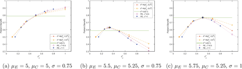
Fig. 1 Total expected average patient benefit for three scenarios, when using a point estimate (dotted lines) and a distribution (normal-dashed lines, uniform-horizontal line) on the prior treatment effect for total patient population N = 500.

In the null scenario, where there is no difference in means for the two treatments, we label the control treatment as “best.” Even though the two treatments result in equal outcomes on average, in this rare disease setting there is unlikely to be an active standard of care treatment and, hence, no side effects from the control treatment. If the patients were to receive an active treatment with no better effect, they would have an increase in risk of side effects and an increase in risk of side effects and the cost of treatment would increase, with no benefit to the patient.

As the null scenario has no difference in treatment means, it only needs a small sample size to (correctly) fail to reject the null hypothesis and allocate all patients outside the trial to the control treatment. Thus, as the sample size, n increases the TEAVPB in the null scenario decreases. Due to both treatments having a normally distributed outcome, the individual variation between patients is symmetric, this along with the mean outcomes being equal implies the TEIPB should always be 0.5 for the null scenario. No matter which treatment a patient is assigned there will always be a 50% chance it will be their individual “best” treatment.

We use numerical optimization methods such as the function “fminbnd” (fminbnd 2016) in matlab (MATLAB 2016) to find the optimal sample size, $n^{\ast }$, which maximizes the TEAVPB, $E[A{B}_N|n,\delta ,\sigma ,\alpha ]$, and the TEIPB, $E[I{B}_N|n,\delta ,\sigma ,\alpha ]$, for six scenarios shown in Table 1.

Table 1 Optimal sample sizes and the total expected patient benefit and power they produce in six scenarios for patient population N = 500.

Scenario				$n^{\ast }$ for	$n^{\ast }$ for	TEAVPB	TEIPB	Power
μE	μC	σ	θ	TEAVPB	TEIPB	for $n^{\ast }$	for $n^{\ast }$	for $n^{\ast }$
5	5	0.75	0	1	–	0.9750	0.5000	–
5.5	5.25	0.75	$\frac{1}{3}$	283	283	0.6305	0.5243	0.8006
5.75	5.25	1	$\frac{1}{2}$	183	183	0.7679	0.5740	0.9225
5.75	5.25	0.75	$\frac{2}{3}$	125	125	0.8460	0.6255	0.9614
6	5	1	1	68	68	0.9188	0.7179	0.9847
6	5	0.75	$\frac{4}{3}$	43	43	0.9497	0.7942	0.9921

In Table 1, the individual optimal sample size is left blank for scenario 1, as the sample size does not make a difference to the TEIPB in this scenario. For the different scenarios above, the optimal sample size varies. However, Table 1 does show the same optimal sample sizes for both TEAVPB and TEIPB for all scenarios and, Figure S1 in the supplementary materials 1.1, shows that the TEAVPB and TEIPB follow the same pattern. This is due to the normally distributed outcome which implies that the individual variation between patients is symmetric about the average response of each treatment. Hence, the definition of patient benefit does not make a difference to the optimal sample size. This is true for all trial designs investigated. However, this may not be the case when a nonsymmetric outcome is considered or when patient’s covariate value(s) affect the outcome of the treatments (see Section 5).

We also find that the clinical trials that use these optimal sample sizes have high power (often well over 80%) in addition to resulting in the maximum patient benefit overall.

3.2 Point Estimate Method: Deviation from Assumptions

The method above finds the TEAVPB and TEIPB for all scenarios when our initial assumptions of ${\mu }_C^{\ast }={\mu }_C,{\mu }_E^{\ast }={\mu }_E$, and ${\sigma }^{\ast }=\sigma$ are correct. As this will rarely be the case we also explore the TEAVPB when our initial assumptions (or priors) of the treatment mean outcomes, ${\mu }_C^{\ast },{\mu }_E^{\ast }$ and standard deviation, ${\sigma }^{\ast }$, are incorrect.

We investigate the TEAVPB for different scenarios with various initial priors on the treatment outcome parameters, ${\mu }_C^{\ast },{\mu }_E^{\ast }$ and ${\sigma }^{\ast }$. We substitute these priors into Equation (5)(5) $$\begin{array}{c}E\left[A{B}_N\right|n,\delta ,\sigma ,\alpha ]\\ \hspace{1em}=\frac{1}{N}(\frac{n}{2}+(N-n)·\Phi (\sqrt{\frac{n·{\delta }^2}{4·{\sigma }^2}}-{\Phi }^{-1}(1-\alpha ))).\hspace{1em}\end{array}$$(5) to find the optimal sample size, $n^{\ast }$, and then use these optimal sample sizes to find the TEAVPB for the actual treatment outcome parameters, μC, μE, and σ in each scenario. The results are shown by the dotted lines in Figure 1 in section 3.3 while additional scenarios are provided in the supplementary materials 1.2. The black 5 pointed stars show the maximum TEAVPB, when the correct values are used as priors: ${\mu }_E^{\ast }={\mu }_E,{\mu }_C^{\ast }={\mu }_C$ and ${\sigma }^{\ast }=\sigma$.

In the null scenario, the largest difference in prior means, ${\delta }^{\ast }={\mu }_E^{\ast }-{\mu }_C^{\ast }$, coupled with the smallest prior standard deviation, ${\sigma }^{\ast }$, produces the largest TEAVPB. This is because it produces the smallest optimal sample size and the null scenario only needs a small sample size to fail to reject the null hypothesis and thus, give all patients outside the trial the control treatment. When the true treatment effect is nonzero, $\theta =({\mu }_E-{\mu }_C)/\sigma \ne 0$, Figure S2 in the supplementary materials 1.2, shows as the prior standard deviation, ${\sigma }^{\ast }$, increases, the prior difference in means, ${\delta }^{\ast }$, which produces the largest patient benefit, also increases. Therefore, if the prior standard deviation, ${\sigma }^{\ast }$, is too high, a large patient benefit can still be produced if an optimistic prior difference in means, ${\delta }^{\ast }$, is also used. The added bonus of using a large prior standard deviation is it produces a trial with larger power, shown in Figure S3 in the supplementary materials 1.2.

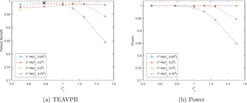
Fig. 2 Total expected average patient benefit (a) and power (b) for trial in case study, when using a distribution on the prior treatment effect for total patient population N = 6680.

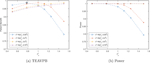
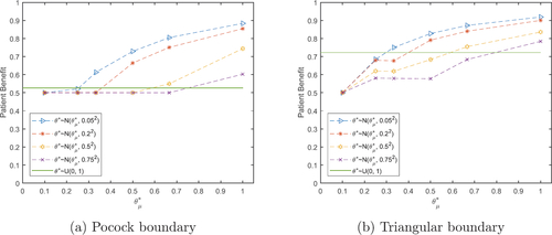
Fig. 3 Total expected average patient benefit for the null scenario (${\mu }_E=5,{\mu }_C=5,\sigma =0.75$) with Pocock (a) and triangular (b) boundaries, when using a distribution on the prior treatment effect for total patient population N = 500.

If the initial assumptions on the treatment outcome parameters: ${\mu }_C^{\ast },{\mu }_E^{\ast }$, and ${\sigma }^{\ast }$ are incorrect, we soon start to see a rapid decrease in TEAVPB highlighting the lack of robustness of the point estimate method.

3.3 Adding Uncertainty in the Treatment Effect

To extend the ideas described by Kaptein (2019) and in order to combat the lack of robustness in the point estimate method, we introduce a distribution on the prior treatment effect, ${\theta }^{\ast }={\delta }^{\ast }/{\sigma }^{\ast }$, instead of using a single prior value on each treatment parameter: ${\mu }_C^{\ast },{\mu }_E^{\ast }$, and ${\sigma }^{\ast }$. The fraction, $\delta /\sigma$ in Equations (5)(5) $$\begin{array}{c}E\left[A{B}_N\right|n,\delta ,\sigma ,\alpha ]\\ \hspace{1em}=\frac{1}{N}(\frac{n}{2}+(N-n)·\Phi (\sqrt{\frac{n·{\delta }^2}{4·{\sigma }^2}}-{\Phi }^{-1}(1-\alpha ))).\hspace{1em}\end{array}$$(5) and (6)(6) $$\begin{array}{c}E\left[I{B}_N\right|n,\delta ,\sigma ,\alpha ]=\frac{1}{N}(\frac{n}{2}\\ \hspace{1em}+(N-n)[\Phi (\sqrt{\frac{n·{\delta }^2}{4·{\sigma }^2}}-{\Phi }^{-1}(1-\alpha ))\\ \hspace{1em}·P(\text{Superior}\mathrm{ }\text{treatment}\mathrm{ }\text{on}\mathrm{ }\text{average}\mathrm{ }\text{is}\mathrm{ }\text{best}\mathrm{ }\text{for}\mathrm{ }\text{patient})\\ \hspace{1em}+(1-\Phi (\sqrt{\frac{n·{\delta }^2}{4·{\sigma }^2}}-{\Phi }^{-1}(1-\alpha )))\\ \hspace{1em}·(1-P(\text{Superior}\mathrm{ }\text{treatment}\mathrm{ }\text{on}\mathrm{ }\text{average}\mathrm{ }\text{is}\mathrm{ }\text{best}\mathrm{ }\text{for}\\ \mathrm{\hspace{1em}}\mathrm{\hspace{1em}}\text{patient}))]).\end{array}$$(6) is replaced with the single term θ, and the TEAVPB and TEIPB are found by taking the expectation over the random variable θ, which is shown in Equations (8)(8) $$\begin{array}{c}E\left[A{B}_N\right|n,\theta ,\alpha ]=E_{\theta }[E\left[A{B}_N\right|n,\theta ,\alpha \left]\right]\\ \hspace{1em}=\frac{1}{N}({\int }_{-\infty }^{\infty }(\frac{1}{{\theta }_{\sigma }\sqrt{2\pi }}\exp (\frac{-{(\theta -{\theta }_{\mu })}^2}{2{\theta }_{\sigma }^2}))\\ \mathrm{\hspace{1em}}\mathrm{\hspace{1em}}·(\frac{n}{2}+(N-n)\Phi (\sqrt{\frac{n{\theta }^2}{4}}-{\Phi }^{-1}(1-\alpha )))d\theta ),\\ \end{array}$$(8) and (9)(9) $$\begin{array}{c}E\left[I{B}_N\right|n,\theta ,\alpha ]=E_{\theta }[E\left[I{B}_N\right|n,\theta ,\alpha \left]\right]\\ \hspace{1em}=\frac{1}{N}({\int }_{-\infty }^{\infty }(\frac{1}{{\theta }_{\sigma }\sqrt{2\pi }}\exp (\frac{-{(\theta -{\theta }_{\mu })}^2}{2{\theta }_{\sigma }^2}))\\ \mathrm{\hspace{1em}}\mathrm{\hspace{1em}}·(\frac{n}{2}+(N-n)[\Phi (\sqrt{\frac{n{\theta }^2}{4}}-{\Phi }^{-1}(1-\alpha ))\\ \mathrm{\hspace{1em}}\mathrm{\hspace{1em}}·P(\text{Superior}\mathrm{ }\text{treatment}\mathrm{ }\text{on}\mathrm{ }\text{average}\mathrm{ }\text{is}\mathrm{ }\text{best}\mathrm{ }\text{for}\mathrm{ }\text{patient})\\ \mathrm{\hspace{1em}}\mathrm{\hspace{1em}}+(1-\Phi (\sqrt{\frac{n{\theta }^2}{4}}-{\Phi }^{-1}(1-\alpha )))\\ \mathrm{\hspace{1em}}\mathrm{\hspace{1em}}·(1-P(\text{Superior}\mathrm{ }\text{treatment}\mathrm{ }\text{on}\mathrm{ }\text{average}\mathrm{ }\text{is}\mathrm{ }\text{best}\mathrm{ }\text{for}\\ \mathrm{\hspace{1em}}\mathrm{\hspace{1em}}\text{patient}))])d\theta ).\end{array}$$(9) ,(8) $$\begin{array}{c}E\left[A{B}_N\right|n,\theta ,\alpha ]=E_{\theta }[E\left[A{B}_N\right|n,\theta ,\alpha \left]\right]\\ \hspace{1em}=\frac{1}{N}({\int }_{-\infty }^{\infty }(\frac{1}{{\theta }_{\sigma }\sqrt{2\pi }}\exp (\frac{-{(\theta -{\theta }_{\mu })}^2}{2{\theta }_{\sigma }^2}))\\ \mathrm{\hspace{1em}}\mathrm{\hspace{1em}}·(\frac{n}{2}+(N-n)\Phi (\sqrt{\frac{n{\theta }^2}{4}}-{\Phi }^{-1}(1-\alpha )))d\theta ),\\ \end{array}$$(8) (9) $$\begin{array}{c}E\left[I{B}_N\right|n,\theta ,\alpha ]=E_{\theta }[E\left[I{B}_N\right|n,\theta ,\alpha \left]\right]\\ \hspace{1em}=\frac{1}{N}({\int }_{-\infty }^{\infty }(\frac{1}{{\theta }_{\sigma }\sqrt{2\pi }}\exp (\frac{-{(\theta -{\theta }_{\mu })}^2}{2{\theta }_{\sigma }^2}))\\ \mathrm{\hspace{1em}}\mathrm{\hspace{1em}}·(\frac{n}{2}+(N-n)[\Phi (\sqrt{\frac{n{\theta }^2}{4}}-{\Phi }^{-1}(1-\alpha ))\\ \mathrm{\hspace{1em}}\mathrm{\hspace{1em}}·P(\text{Superior}\mathrm{ }\text{treatment}\mathrm{ }\text{on}\mathrm{ }\text{average}\mathrm{ }\text{is}\mathrm{ }\text{best}\mathrm{ }\text{for}\mathrm{ }\text{patient})\\ \mathrm{\hspace{1em}}\mathrm{\hspace{1em}}+(1-\Phi (\sqrt{\frac{n{\theta }^2}{4}}-{\Phi }^{-1}(1-\alpha )))\\ \mathrm{\hspace{1em}}\mathrm{\hspace{1em}}·(1-P(\text{Superior}\mathrm{ }\text{treatment}\mathrm{ }\text{on}\mathrm{ }\text{average}\mathrm{ }\text{is}\mathrm{ }\text{best}\mathrm{ }\text{for}\\ \mathrm{\hspace{1em}}\mathrm{\hspace{1em}}\text{patient}))])d\theta ).\end{array}$$(9)

The TEAVPB is investigated for three scenarios with various prior treatment effects which are normally distributed with mean, ${\theta }_{\mu }^{\ast }=\{0.1,0.25,0.333,0.5,0.666,1\}$, and standard deviations, ${\theta }_{\sigma }^{\ast }=\{0.2,0.5\}$, shown by the dashed lines in Figure 1. We further investigate a uniform distribution on the prior treatment effect between 0 and 1 (reported by the horizontal line in Figure 1), where the normal probability distribution, $(1/({\theta }_{\sigma }\sqrt{2\pi }))·\exp (-{(\theta -{\theta }_{\mu })}^2/2{\theta }_{\sigma }^2)$, is replaced with 1 in Equations (8)(8) $$\begin{array}{c}E\left[A{B}_N\right|n,\theta ,\alpha ]=E_{\theta }[E\left[A{B}_N\right|n,\theta ,\alpha \left]\right]\\ \hspace{1em}=\frac{1}{N}({\int }_{-\infty }^{\infty }(\frac{1}{{\theta }_{\sigma }\sqrt{2\pi }}\exp (\frac{-{(\theta -{\theta }_{\mu })}^2}{2{\theta }_{\sigma }^2}))\\ \mathrm{\hspace{1em}}\mathrm{\hspace{1em}}·(\frac{n}{2}+(N-n)\Phi (\sqrt{\frac{n{\theta }^2}{4}}-{\Phi }^{-1}(1-\alpha )))d\theta ),\\ \end{array}$$(8) and (9)(9) $$\begin{array}{c}E\left[I{B}_N\right|n,\theta ,\alpha ]=E_{\theta }[E\left[I{B}_N\right|n,\theta ,\alpha \left]\right]\\ \hspace{1em}=\frac{1}{N}({\int }_{-\infty }^{\infty }(\frac{1}{{\theta }_{\sigma }\sqrt{2\pi }}\exp (\frac{-{(\theta -{\theta }_{\mu })}^2}{2{\theta }_{\sigma }^2}))\\ \mathrm{\hspace{1em}}\mathrm{\hspace{1em}}·(\frac{n}{2}+(N-n)[\Phi (\sqrt{\frac{n{\theta }^2}{4}}-{\Phi }^{-1}(1-\alpha ))\\ \mathrm{\hspace{1em}}\mathrm{\hspace{1em}}·P(\text{Superior}\mathrm{ }\text{treatment}\mathrm{ }\text{on}\mathrm{ }\text{average}\mathrm{ }\text{is}\mathrm{ }\text{best}\mathrm{ }\text{for}\mathrm{ }\text{patient})\\ \mathrm{\hspace{1em}}\mathrm{\hspace{1em}}+(1-\Phi (\sqrt{\frac{n{\theta }^2}{4}}-{\Phi }^{-1}(1-\alpha )))\\ \mathrm{\hspace{1em}}\mathrm{\hspace{1em}}·(1-P(\text{Superior}\mathrm{ }\text{treatment}\mathrm{ }\text{on}\mathrm{ }\text{average}\mathrm{ }\text{is}\mathrm{ }\text{best}\mathrm{ }\text{for}\\ \mathrm{\hspace{1em}}\mathrm{\hspace{1em}}\text{patient}))])d\theta ).\end{array}$$(9) . These priors are used to find the optimal sample size, $n^{\ast }$, and then the optimal sample size is used to find the TEAVPB for the actual treatment outcome parameters: μC, μE, and σ in each scenario.

In the null scenario, the largest prior treatment effect mean, ${\theta }_{\mu }^{\ast }$, coupled with the smallest prior treatment effect standard deviation, ${\theta }_{\sigma }^{\ast }$, produces the larger TEAVPB. Here, using the point estimate prior on each outcome parameter, performs better than using a normal distribution on the prior treatment effect. Specifically, when the point estimate method is used with the priors: ${\mu }_E^{\ast }=5.75$, ${\mu }_C^{\ast }=5.25$, and ${\sigma }^{\ast }=0.5$, the TEAVPB = 0.9104 is found when the treatment effect is actually ${\mu }_E={\mu }_C=5$. However, when we use a normal distribution on the prior treatment effect: ${\theta }_{\mu }^{\ast }=({\mu }_E^{\ast }-{\mu }_C^{\ast })/{\sigma }^{\ast }=(5.75-5.25)/0.5=1$ with treatment effect standard deviation ${\theta }_{\sigma }^{\ast }=0.5$, the TEAVPB = 0.8800. Thus, the point estimate prior results in a TEAVPB, which is larger than using a normal distribution prior on the treatment effect by 0.0304. However, this gain in the null scenario comes at a loss when the treatment effect is nonzero, shown in Figures 1(b)–(c).

In Figures 1(b)–(c), when the treatment effect prior mean, ${\theta }_{\mu }^{\ast }$, is smaller than the true treatment effect, θ, the value of its prior standard deviation, ${\theta }_{\sigma }^{\ast }$, does not have a large effect on the TEAVPB produced and both methods produce similar patient benefit. As the prior, ${\theta }_{\mu }^{\ast }$, increases past the true mean, it is the smaller prior treatment effect standard deviations, ${\theta }_{\sigma }^{\ast }$, which cause a quicker decrease in TEAVPB. Here, using a normal distribution on the prior treatment effect is more robust than the point estimate prior. Specifically, when a normal distribution with prior mean ${\theta }_{\mu }^{\ast }=({\mu }_E^{\ast }-{\mu }_C^{\ast })/{\sigma }^{\ast }=(5.75-5.25)/0.5=1$ and prior standard deviation ${\theta }_{\sigma }^{\ast }=0.5$ are used, the TEAVPB = 0.6643, when the true treatment effect is $\theta =({\mu }_E-{\mu }_C)/\sigma =(5.75-5.25)/1=0.5$. However, when the point estimate method is used with priors: ${\mu }_E^{\ast }=5.75,{\mu }_C^{\ast }=5.25$, and ${\sigma }^{\ast }=0.5$, the TEAVPB = 0.5350. Hence, the prior point estimate method results in a TEAVPB, which is smaller than using a normal distribution on the prior treatment effect by 0.1293. Introducing a uniform distribution on the prior treatment effect performs well in Figures 1(b)–(c), giving a TEAVPB close to the maximum value. However, using a uniform distribution on the prior treatment effect will struggle in the null scenario. A further three scenarios are explored in Figure S4 in the supplementary materials 1.3. In addition, Figure S5 in the supplementary materials 1.3, shows the power is largest for the larger values of ${\theta }_{\sigma }^{\ast }$. Furthermore, using a distribution on the prior treatment effect produces a larger power than using the prior point estimate method.

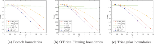
Fig. 4 Total expected average patient benefit averaged across all six scenarios, when using a point estimate (dotted lines) and a distribution (normal-dashed lines, uniform-horizontal lines) on the prior treatment effect, with Pocock (a), O’Brien Fleming (b) and triangular (c) boundaries, for total patient population N = 500.

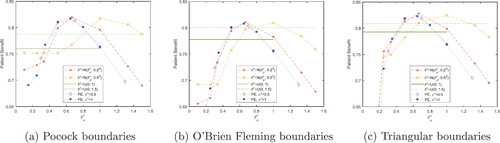
Fig. 5 Power averaged across all six scenarios, when using a point estimate (dotted lines) and a distribution (normal-dashed lines, uniform-horizontal lines) on the prior treatment effect, with Pocock (a), O’Brien Fleming (b) and triangular (c) boundaries, for total patient population N = 500.

3.4 Case Study Results

Equation (5)(5) $$\begin{array}{c}E\left[A{B}_N\right|n,\delta ,\sigma ,\alpha ]\\ \hspace{1em}=\frac{1}{N}(\frac{n}{2}+(N-n)·\Phi (\sqrt{\frac{n·{\delta }^2}{4·{\sigma }^2}}-{\Phi }^{-1}(1-\alpha ))).\hspace{1em}\end{array}$$(5) can further be used to find the optimal sample size $n^{\ast }$ to produce the maximum TEAVPB for the case study described in Section 2, using the prior point estimate method. We assume a difference in means of ${\delta }^{\ast }=20.2\%$ and a prior standard deviation of ${\sigma }^{\ast }=18\%$Z${\sigma }^{\ast }=18\%$ to give an optimal sample size of $n^{\ast }=84$, TEAVPB$=0.9930$ and power$=0.9993$. This sample size would actually result in a TEAVPB$=0.9401$ and power$=0.9457$, due to the actual difference between the means in the trial being $\widehat{\delta }=14\%$. When the true difference in means from the trial, ${\delta }^{\ast }=\widehat{\delta }=14\%$, and standard deviation, ${\sigma }^{\ast }=\widehat{\sigma }=18\%$, are used as the point estimate priors, the resulting optimal sample size of $n^{\ast }=160$, gives TEAVPB$=0.9865$ and power$=$ 0.9985.

In addition, Equation (8)(8) $$\begin{array}{c}E\left[A{B}_N\right|n,\theta ,\alpha ]=E_{\theta }[E\left[A{B}_N\right|n,\theta ,\alpha \left]\right]\\ \hspace{1em}=\frac{1}{N}({\int }_{-\infty }^{\infty }(\frac{1}{{\theta }_{\sigma }\sqrt{2\pi }}\exp (\frac{-{(\theta -{\theta }_{\mu })}^2}{2{\theta }_{\sigma }^2}))\\ \mathrm{\hspace{1em}}\mathrm{\hspace{1em}}·(\frac{n}{2}+(N-n)\Phi (\sqrt{\frac{n{\theta }^2}{4}}-{\Phi }^{-1}(1-\alpha )))d\theta ),\\ \end{array}$$(8) is used to find the optimal sample size $n^{\ast }$ to produce the maximum TEAVPB using a distribution on the prior treatment effect, ${\theta }^{\ast }$. We assume a treatment effect which is normally distributed with prior means ${\theta }_{\mu }^{\ast }=\{0.5,0.78,1,1.12,1.25,1.5\}$ and prior standard deviations of ${\theta }_{\sigma }^{\ast }=\{0.05,0.2,0.5,0.75\}$ and investigate the actual TEAV-PB and power produced in the trial with treatment effect $\widehat{\theta }=(96-82)/18=0.778$ (Figure 2).

As seen before, when the prior mean of θ is smaller than the true treatment effect, ${\theta }_{\mu }^{\ast }<\theta$, the value of its prior standard deviation, ${\theta }_{\sigma }^{\ast }$, does not have a large effect on the TEAVPB produced. As ${\theta }_{\mu }^{\ast }$ increases past the true mean, it is the smaller prior standard deviations, ${\theta }_{\sigma }^{\ast }$, which cause a quicker decrease in TEAVPB. When we use our prior treatment effect mean, ${\theta }_{\mu }^{\ast }=20.2/18=1.12$, and moderate prior standard deviation, ${\theta }_{\sigma }^{\ast }=0.2$, we get $n^{\ast }=122$, TEAVPB = 0.9813 and power = 0.9902, (incidentally, these are larger than using the incorrect treatment effect in the point estimate method). Whereas, using the treatment effect from the trial as the prior mean, ${\theta }_{\mu }^{\ast }=\widehat{\theta }=0.78$, and small prior standard deviation, ${\theta }_{\sigma }^{\ast }=0.05$, gives $n^{\ast }=166$, TEAVPB = 0.9865 and power = 0.9989. The difference here is not large and therefore, we can still produce a large TEAVPB even when our initial assumptions about the treatment effect are incorrect.

3.5 The Effect of the Total Patient Population

If the total patient population N decreases, the sample size which maximizes the total patient benefit also decreases. If N is decreased enough, the optimal sample size $n^{\ast }$, will no longer produce a trial with power larger than 80%. When the treatment effect is small and the whole patient population is N = 80, it is actually most beneficial to have everyone in the trial. This can be seen from Figure S6(c) in the supplementary materials 1.4. Here, we use the prior point estimate method with the correct treatment outcome parameters: ${\mu }_C^{\ast }={\mu }_C,{\mu }_E^{\ast }={\mu }_E$ and ${\sigma }^{\ast }=\sigma$ for each scenario. Figure S6, in the supplementary materials 1.4, also displays vertical lines which represent the sample size n needed for a trial to have 80% power, for each scenario.

Fig. 6 Total expected average patient benefit (a) and power (b) for trial in case study, when using Pocock boundaries and a distribution on the prior treatment effect for total patient population N = 6680.

4 Sequential Designs

A sequential design for a clinical trial is described by Whitehead (2002) as an approach which performs a series of analyses throughout the trial, where there is the potential to stop the trial at each analysis. These designs are efficient due to their ability to stop the trial early for either efficacy or futility (Pallmann et al. 2018).

We now seek to optimize a two-stage sequential design (which includes a single interim analysis) using techniques similar to those shown above. We focus on the two-stage design as these are commonly used in clinical trials (Jovic and Whitehead 2010). We investigate the Pocock boundaries (Pocock 1977), O’Brien Fleming boundaries (O’Brien and Fleming 1979) and triangular boundaries (Whitehead and Stratton 1983).

In a two-stage design, the trial is stopped after the first stage for efficacy, if the test statistic, Z1, is larger than the first stage upper boundary, $B_{1,u}$. The trial is stopped for futility after the first stage, if the test statistic, Z1, is smaller than the first stage lower boundary, $B_{1,l}$. And, hence, the trial reaches the second stage if the test statistic, Z1, is between $B_{1,l}$ and $B_{1,u}$.

If the trial is stopped after stage one for efficacy, then all patients outside stage one, $N-n_1$, will receive the experimental treatment. If the trial is stopped after stage one for futility then all patients outside stage one, $N-n_1$, will receive the control treatment.

After the second stage has been completed, the Z-test is used to determine if the null hypothesis should be rejected. This time the null hypothesis is rejected if the test statistic, Z2, is larger than the second stage boundary, B2, and thus, all patients outside stage one and stage two, $N-n_1-n_2$, will receive the experimental treatment. If the null hypothesis is not rejected after the second stage all patients outside stage one and stage two, $N-n_1-n_2$, will receive the control treatment.

Thus, given we know the distributions of the patient outcomes, the TEAVPB is(10) $$\begin{array}{c}E\left[A{B}_N\right|n_1,n_2,\delta ,\sigma ,\alpha ]\\ \hspace{1em}=\frac{1}{N}(\mathrm{}\frac{n_1}{2}+(N-n_1)P(B_{1,u}\le Z_1)\\ \mathrm{\hspace{1em}}\mathrm{\hspace{1em}}+ \frac{n_2}{2}P(B_{1,l}\le Z_1<B_{1,u})\\ \mathrm{\hspace{1em}}\mathrm{\hspace{1em}}+ (N-n_1-n_2)P(B_{1,l}\le Z_1<B_{1,u},B_2\le Z_2)\mathrm{}).\hspace{1em}\end{array}$$(10)

Here, Z1 and Z2 represent Z-test statistics calculated from the trial after the first and second stage of the trial has been completed. Hence, $Z_1=\delta /\sqrt{2{\sigma }^2/\frac{n_1}{2}}$ and $Z_2=\delta /\sqrt{2{\sigma }^2/\frac{n_1+n_2}{2}}$, where δ is the difference between the two treatment means and σ is the common standard deviation of the outcome for both treatments. Furthermore, $B_{1,l}$ and $B_{1,u}$ represent the lower and upper boundaries for stage 1 and B2 represents the boundary for stage 2.

For the TEIPB, we have the added issue that the superior treatment on average, may not be an individual’s superior treatment. Thus, Equation (10)(10) $$\begin{array}{c}E\left[A{B}_N\right|n_1,n_2,\delta ,\sigma ,\alpha ]\\ \hspace{1em}=\frac{1}{N}(\mathrm{}\frac{n_1}{2}+(N-n_1)P(B_{1,u}\le Z_1)\\ \mathrm{\hspace{1em}}\mathrm{\hspace{1em}}+ \frac{n_2}{2}P(B_{1,l}\le Z_1<B_{1,u})\\ \mathrm{\hspace{1em}}\mathrm{\hspace{1em}}+ (N-n_1-n_2)P(B_{1,l}\le Z_1<B_{1,u},B_2\le Z_2)\mathrm{}).\hspace{1em}\end{array}$$(10) changes to incorporate this, as shown in Equation (11)(11) $$\begin{array}{c}E\left[I{B}_N\right|n_1,n_2,\delta ,\sigma ,\alpha ]=\frac{1}{N}(\frac{n_1}{2}\\ \hspace{1em}+ (N-n_1)[P(B_{1,u}\le Z_1)P(\text{Superior}\mathrm{ }\text{treatment}\mathrm{ }\text{on}\mathrm{ }\text{average}\\ \mathrm{\hspace{1em}}\mathrm{\hspace{1em}}\text{is}\mathrm{ }\text{best}\mathrm{ }\text{for}\mathrm{ }\text{patient})\\ \hspace{1em}+ P(B_{1,l}>Z_1)(1-P(\text{Superior}\mathrm{ }\text{treatment}\mathrm{ }\text{on}\mathrm{ }\text{average}\mathrm{ }\text{is}\\ \mathrm{\hspace{1em}}\mathrm{\hspace{1em}}\text{best}\mathrm{ }\text{for}\mathrm{ }\text{patient}))]\\ \hspace{1em}+ \frac{n_2}{2}P(B_{1,l}\le Z_1<B_{1,u})\\ \hspace{1em}+ (N-n_1-n_2)[P(B_{1,l}\le Z_1<B_{1,u},B_2\le Z_2)\\ \hspace{1em}· P(\text{Superior}\mathrm{ }\text{treatment}\mathrm{ }\text{on}\mathrm{ }\text{average}\mathrm{ }\text{is}\mathrm{ }\text{best}\mathrm{ }\text{for}\mathrm{ }\text{patient})\\ \hspace{1em}+ P(B_{1,l}\le Z_1<B_{1,u},B_2>Z_2)\\ \hspace{1em}· (1-P(\text{Superior}\mathrm{ }\text{treatment}\mathrm{ }\text{on}\mathrm{ }\text{average}\mathrm{ }\text{is}\mathrm{ }\text{best}\mathrm{ }\text{for}\\ \mathrm{\hspace{1em}}\mathrm{\hspace{1em}}\text{patient}))]).\end{array}$$(11) ,(11) $$\begin{array}{c}E\left[I{B}_N\right|n_1,n_2,\delta ,\sigma ,\alpha ]=\frac{1}{N}(\frac{n_1}{2}\\ \hspace{1em}+ (N-n_1)[P(B_{1,u}\le Z_1)P(\text{Superior}\mathrm{ }\text{treatment}\mathrm{ }\text{on}\mathrm{ }\text{average}\\ \mathrm{\hspace{1em}}\mathrm{\hspace{1em}}\text{is}\mathrm{ }\text{best}\mathrm{ }\text{for}\mathrm{ }\text{patient})\\ \hspace{1em}+ P(B_{1,l}>Z_1)(1-P(\text{Superior}\mathrm{ }\text{treatment}\mathrm{ }\text{on}\mathrm{ }\text{average}\mathrm{ }\text{is}\\ \mathrm{\hspace{1em}}\mathrm{\hspace{1em}}\text{best}\mathrm{ }\text{for}\mathrm{ }\text{patient}))]\\ \hspace{1em}+ \frac{n_2}{2}P(B_{1,l}\le Z_1<B_{1,u})\\ \hspace{1em}+ (N-n_1-n_2)[P(B_{1,l}\le Z_1<B_{1,u},B_2\le Z_2)\\ \hspace{1em}· P(\text{Superior}\mathrm{ }\text{treatment}\mathrm{ }\text{on}\mathrm{ }\text{average}\mathrm{ }\text{is}\mathrm{ }\text{best}\mathrm{ }\text{for}\mathrm{ }\text{patient})\\ \hspace{1em}+ P(B_{1,l}\le Z_1<B_{1,u},B_2>Z_2)\\ \hspace{1em}· (1-P(\text{Superior}\mathrm{ }\text{treatment}\mathrm{ }\text{on}\mathrm{ }\text{average}\mathrm{ }\text{is}\mathrm{ }\text{best}\mathrm{ }\text{for}\\ \mathrm{\hspace{1em}}\mathrm{\hspace{1em}}\text{patient}))]).\end{array}$$(11)

The probabilities from Equations (10)(10) $$\begin{array}{c}E\left[A{B}_N\right|n_1,n_2,\delta ,\sigma ,\alpha ]\\ \hspace{1em}=\frac{1}{N}(\mathrm{}\frac{n_1}{2}+(N-n_1)P(B_{1,u}\le Z_1)\\ \mathrm{\hspace{1em}}\mathrm{\hspace{1em}}+ \frac{n_2}{2}P(B_{1,l}\le Z_1<B_{1,u})\\ \mathrm{\hspace{1em}}\mathrm{\hspace{1em}}+ (N-n_1-n_2)P(B_{1,l}\le Z_1<B_{1,u},B_2\le Z_2)\mathrm{}).\hspace{1em}\end{array}$$(10) and (11)(11) $$\begin{array}{c}E\left[I{B}_N\right|n_1,n_2,\delta ,\sigma ,\alpha ]=\frac{1}{N}(\frac{n_1}{2}\\ \hspace{1em}+ (N-n_1)[P(B_{1,u}\le Z_1)P(\text{Superior}\mathrm{ }\text{treatment}\mathrm{ }\text{on}\mathrm{ }\text{average}\\ \mathrm{\hspace{1em}}\mathrm{\hspace{1em}}\text{is}\mathrm{ }\text{best}\mathrm{ }\text{for}\mathrm{ }\text{patient})\\ \hspace{1em}+ P(B_{1,l}>Z_1)(1-P(\text{Superior}\mathrm{ }\text{treatment}\mathrm{ }\text{on}\mathrm{ }\text{average}\mathrm{ }\text{is}\\ \mathrm{\hspace{1em}}\mathrm{\hspace{1em}}\text{best}\mathrm{ }\text{for}\mathrm{ }\text{patient}))]\\ \hspace{1em}+ \frac{n_2}{2}P(B_{1,l}\le Z_1<B_{1,u})\\ \hspace{1em}+ (N-n_1-n_2)[P(B_{1,l}\le Z_1<B_{1,u},B_2\le Z_2)\\ \hspace{1em}· P(\text{Superior}\mathrm{ }\text{treatment}\mathrm{ }\text{on}\mathrm{ }\text{average}\mathrm{ }\text{is}\mathrm{ }\text{best}\mathrm{ }\text{for}\mathrm{ }\text{patient})\\ \hspace{1em}+ P(B_{1,l}\le Z_1<B_{1,u},B_2>Z_2)\\ \hspace{1em}· (1-P(\text{Superior}\mathrm{ }\text{treatment}\mathrm{ }\text{on}\mathrm{ }\text{average}\mathrm{ }\text{is}\mathrm{ }\text{best}\mathrm{ }\text{for}\\ \mathrm{\hspace{1em}}\mathrm{\hspace{1em}}\text{patient}))]).\end{array}$$(11) are defined below,$$\begin{array}{c}P(B_{1,u}\le Z_1)=\Phi (\frac{\delta \sqrt{n_1}}{2\sigma }-B_{1,u}),\\ P(B_{1,l}\le Z_1<B_{1,u})=\Phi (\frac{\delta \sqrt{n_1}}{2\sigma }-B_{1,l})\\ \mathrm{\hspace{1em}}\mathrm{\hspace{1em}}-\Phi (\frac{\delta \sqrt{n_1}}{2\sigma }-B_{1,u}),\\ P(B_{1,l}\le Z_1<B_{1,u},B_2\le Z_2)\\ \hspace{1em}={\Phi }_2(\frac{\delta \sqrt{n_1}}{2\sigma }-B_{1,l},\frac{\delta \sqrt{n_1+n_2}}{2\sigma }-B_2,\Sigma )\\ \mathrm{\hspace{1em}}\mathrm{\hspace{1em}}-{\Phi }_2(\frac{\delta \sqrt{n_1}}{2\sigma }-B_{1,u},\frac{\delta \sqrt{n_1+n_2}}{2\sigma }-B_2,\Sigma ),\\ \Sigma =\left[\begin{array}{cc}1& \sqrt{\frac{n_1}{n_1+n_2}}\\ \sqrt{\frac{n_1}{n_1+n_2}}& 1\end{array}\right].\end{array}$$

Here, $\Phi (x_1)$ is the normal cumulative distribution, $P(x_1\le X_1)$ and ${\Phi }_2(x_1,x_2,\Sigma )$ is the bivariate normal cumulative distribution, $P(x_1\le X_1,x_2\le X_2)$ and Σ is the covariance matrix for X1 and X2. The boundaries $B_{1,l},B_{1,u}$, and B2, vary depending on the shape of the boundary and the chosen Type I error, α.

4.1 Point Estimate Method

We investigate the total expected patient benefit produced using Equations (10)(10) $$\begin{array}{c}E\left[A{B}_N\right|n_1,n_2,\delta ,\sigma ,\alpha ]\\ \hspace{1em}=\frac{1}{N}(\mathrm{}\frac{n_1}{2}+(N-n_1)P(B_{1,u}\le Z_1)\\ \mathrm{\hspace{1em}}\mathrm{\hspace{1em}}+ \frac{n_2}{2}P(B_{1,l}\le Z_1<B_{1,u})\\ \mathrm{\hspace{1em}}\mathrm{\hspace{1em}}+ (N-n_1-n_2)P(B_{1,l}\le Z_1<B_{1,u},B_2\le Z_2)\mathrm{}).\hspace{1em}\end{array}$$(10) , (11)(11) $$\begin{array}{c}E\left[I{B}_N\right|n_1,n_2,\delta ,\sigma ,\alpha ]=\frac{1}{N}(\frac{n_1}{2}\\ \hspace{1em}+ (N-n_1)[P(B_{1,u}\le Z_1)P(\text{Superior}\mathrm{ }\text{treatment}\mathrm{ }\text{on}\mathrm{ }\text{average}\\ \mathrm{\hspace{1em}}\mathrm{\hspace{1em}}\text{is}\mathrm{ }\text{best}\mathrm{ }\text{for}\mathrm{ }\text{patient})\\ \hspace{1em}+ P(B_{1,l}>Z_1)(1-P(\text{Superior}\mathrm{ }\text{treatment}\mathrm{ }\text{on}\mathrm{ }\text{average}\mathrm{ }\text{is}\\ \mathrm{\hspace{1em}}\mathrm{\hspace{1em}}\text{best}\mathrm{ }\text{for}\mathrm{ }\text{patient}))]\\ \hspace{1em}+ \frac{n_2}{2}P(B_{1,l}\le Z_1<B_{1,u})\\ \hspace{1em}+ (N-n_1-n_2)[P(B_{1,l}\le Z_1<B_{1,u},B_2\le Z_2)\\ \hspace{1em}· P(\text{Superior}\mathrm{ }\text{treatment}\mathrm{ }\text{on}\mathrm{ }\text{average}\mathrm{ }\text{is}\mathrm{ }\text{best}\mathrm{ }\text{for}\mathrm{ }\text{patient})\\ \hspace{1em}+ P(B_{1,l}\le Z_1<B_{1,u},B_2>Z_2)\\ \hspace{1em}· (1-P(\text{Superior}\mathrm{ }\text{treatment}\mathrm{ }\text{on}\mathrm{ }\text{average}\mathrm{ }\text{is}\mathrm{ }\text{best}\mathrm{ }\text{for}\\ \mathrm{\hspace{1em}}\mathrm{\hspace{1em}}\text{patient}))]).\end{array}$$(11) , and (7)(7) $$P(Y_E>Y_C)=1-P(Y_E-Y_C<\frac{-({\mu }_E-{\mu }_C)}{\sqrt{2{\sigma }^2}}).$$(7) in a two-stage design. The average response from two treatment arms, a control and an experimental treatment, are compared using a Z-test where the variance is assumed equal. Additionally, the Type I error is chosen to be $\alpha =0.05$ and the patient population is N = 500, to reflect the context of rare disease trials. The TEAVPB and TEIPB are investigated for a number of sample sizes, where $n_1^{\ast }=n_2^{\ast }$, shown in Figure S7 in the supplementary materials 2.

Numerical optimization methods such as the function “fminbnd” (fminbnd 2016) (when we assume $n_1=n_2$) and “fmincon” (fmincon 2016) (when we assume $n_1\ne n_2$) in matlab (MATLAB 2016) are used to find the optimal sample sizes of the first stage, $n_1^{\ast }$, and the second stage, $n_2^{\ast }$, of the trial, which maximizes the TEAVPB, $E[A{B}_N|n_1,n_2,\delta ,\sigma ,\alpha ]$, and TEIPB, $E[I{B}_N|n_1,n_2,\delta ,\sigma ,\alpha ]$, in each scenario for each boundary. These are listed in Table A.1 in Appendix A, where $n_1^{\ast }=n_2^{\ast }$.

Table A.1 Optimal sample sizes, total expected average patient benefit, expected sample sizes and power they produce in six scenarios for a two-stage design with Pocock, O’Brien Fleming and triangular boundaries for total patient population N = 500.

Boundary	Scenario				$n_1^{\ast }$	TEAVPB	$P(\text{stop}\mathrm{ }\text{after}$	$E[n^{\ast }]$	Power
	μE	μC	σ	θ			$\text{first}\mathrm{ }\text{stage})$		for $n_1^{\ast }$
Pocock	5	5	0.75	0	1	0.9731	0.0294	2	–
	5.5	5.25	0.75	$\frac{1}{3}$	186	0.6932	0.5377	272	0.8642
	5.75	5.25	1	$\frac{1}{2}$	122	0.8246	0.7201	156	0.9624
	5.75	5.25	0.75	$\frac{2}{3}$	82	0.8907	0.7996	98	0.9838
	6	5	1	1	43	0.9461	0.8644	49	0.9939
	6	5	0.75	$\frac{4}{3}$	27	0.9678	0.9007	30	0.9971
O’Brien Fleming	5	5	0.75	0	1	0.9731	0.0052	2	–
	5.5	5.25	0.75	$\frac{1}{3}$	160	0.6631	0.2456	281	0.8438
	5.75	5.25	1	$\frac{1}{2}$	108	0.8043	0.4214	170	0.9556
	5.75	5.25	0.75	$\frac{2}{3}$	75	0.8780	0.536	110	0.9826
	6	5	1	1	41	0.9405	0.6573	55	0.9947
	6	5	0.75	$\frac{4}{3}$	25	0.9649	0.7043	32	0.9969
Triangular	5	5	0.75	0	1	0.9739	0.7837	1	–
	5.5	5.25	0.75	$\frac{1}{3}$	192	0.6765	0.5932	270	0.8663
	5.75	5.25	1	$\frac{1}{2}$	126	0.8169	0.7399	159	0.9608
	5.75	5.25	0.75	$\frac{2}{3}$	85	0.8856	0.8125	101	0.9821
	6	5	1	1	45	0.9431	0.8757	51	0.9928
	6	5	0.75	$\frac{4}{3}$	28	0.9657	0.9068	31	0.9961

The optimal sample sizes when $n_1^{\ast }\ne n_2^{\ast }$, which maximize the TEAVPB, $E[A{B}_N|n_1,n_2,\delta ,$ $\sigma ,\alpha ]$, and the TEIPB, $E[I{B}_N|n_1,n_2,\delta ,\sigma ,\alpha ]$, for each scenario are displayed in Tables 2–4 in the supplementary materials 2.1.1, 2.2.1, and 2.3.1, respectively.

4.2 Adding Uncertainty in the Treatment Effect

Additionally, we can explore this two-stage design using a distribution on the prior treatment effect, instead of the prior point estimate method used above. We investigate a normal distribution on θ with prior means ${\theta }_{\mu }^{\ast }=\{0.1,0.25,0.333,0.5,0.666,1\}$ and prior standard deviations ${\theta }_{\sigma }^{\ast }=\{0.05,0.2,0.5,0.75\}$ and a prior uniform distribution between 0 and 1. Figure 3 displays the TEAVPB for the null scenario, using the Pocock and triangular boundaries.

Figure 3 shows, as the prior mean of θ increases from ${\theta }_{\mu }^{\ast }=0.1$, the TEAVPB increases. The larger the prior mean of θ, the closer the sample sizes get to the true optimal sample sizes $n_1^{*}=n_2^{*}=1$. Also, the smaller the prior treatment effect standard deviation, ${\theta }_{\sigma }^{\ast }$, again the smaller the sample sizes and the larger the TEAVPB. The triangular boundaries produce a larger TEAVPB than the Pocock boundaries for the corresponding prior means and standard deviations of θ. In the null scenario the uniform distribution does not perform well and often produces a lower patient benefit than the normal distributions investigated. It makes sense that the triangular boundaries come out on top for the null scenario, as these boundaries have the most aggressive stopping probability when there is little difference between the two treatments.

The optimal sample sizes of both stages, $n_1^{\ast }$ and $n_2^{\ast }$, are found for all three boundaries in the supplementary materials. These optimal sample sizes are then substituted into Equation (10)(10) $$\begin{array}{c}E\left[A{B}_N\right|n_1,n_2,\delta ,\sigma ,\alpha ]\\ \hspace{1em}=\frac{1}{N}(\mathrm{}\frac{n_1}{2}+(N-n_1)P(B_{1,u}\le Z_1)\\ \mathrm{\hspace{1em}}\mathrm{\hspace{1em}}+ \frac{n_2}{2}P(B_{1,l}\le Z_1<B_{1,u})\\ \mathrm{\hspace{1em}}\mathrm{\hspace{1em}}+ (N-n_1-n_2)P(B_{1,l}\le Z_1<B_{1,u},B_2\le Z_2)\mathrm{}).\hspace{1em}\end{array}$$(10) to find the TEAVPB for all six scenarios. This is shown in Figures S9, S12, and S15 and the power is shown in Figures S10, S13, and S16 for Pocock, O’Brien Fleming and Triangular boundaries in the supplementary materials 2.1.2, 2.2.2, and 2.3.2, respectively.

When the true treatment effect is nonzero, the patient benefit tends to be fairly large when the prior mean of θ is small. Then as the prior mean of θ increases, the patient benefit starts to decrease. This decrease starts at smaller values of ${\theta }_{\mu }^{\ast }$ for the smaller values of the prior standard deviation of θ. The TEAVPB is fairly robust when ${\theta }_{\sigma }^{\ast }$ is large. When the true treatment effect is nonzero, the uniform distribution performs well and often produces a larger patient benefit than the normal distributions investigated.

The power of the trial decreases as the prior mean of θ increases and as the prior standard deviation of θ decreases. This is due to the sample sizes decreasing in these situations and hence, the power decreases.

Figure 3(a) highlights the main issue with using ${\theta }^{\ast } \sim U(0,1)$. Even though it is robust and gives large patient benefit for scenarios with a nonzero treatment effect, the risk of using this distribution is too great. In application many clinical trials find no difference between the two treatments and therefore, the null scenario is most important in regards to the application. In the null scenario, the potential loss in patient benefit is very large.

To find out which method (using a point estimate prior (PE), ${\mu }_E^{\ast },{\mu }_C^{\ast }$, and ${\sigma }^{\ast }$, uniform distribution for prior treatment effect ${\theta }^{\ast }$ or normal distribution for prior treatment effect ${\theta }^{\ast }$) and which prior values for the treatment effect performed best, the TEAVPB and power were averaged across all six scenarios, for all three boundaries. The results for TEAVPB are shown in Figure 4 and the results for power are shown in Figure 5.

These plots show that the boundary that comes out on top across the majority of methods and treatment effect assumptions, is triangular. This is due to its superiority in the null scenario, outweighing its slight inferiority in the other scenarios. The assumed distribution on the prior treatment effect ${\theta }^{\ast }\sim N(2/3,{0.2}^2)$ produces the largest TEAVPB averaged across all scenarios. This distribution also gives an average power of 0.9244, which is very high. Traditionally, clinical trial designs should guarantee a power of at least 0.8. Our best method which maximizes TEAVPB, also gives an average power above 0.8 and therefore, this method could be applicable in a real clinical trial.

4.3 Case Study Results

The prior point estimate method is used with Equation (10)(10) $$\begin{array}{c}E\left[A{B}_N\right|n_1,n_2,\delta ,\sigma ,\alpha ]\\ \hspace{1em}=\frac{1}{N}(\mathrm{}\frac{n_1}{2}+(N-n_1)P(B_{1,u}\le Z_1)\\ \mathrm{\hspace{1em}}\mathrm{\hspace{1em}}+ \frac{n_2}{2}P(B_{1,l}\le Z_1<B_{1,u})\\ \mathrm{\hspace{1em}}\mathrm{\hspace{1em}}+ (N-n_1-n_2)P(B_{1,l}\le Z_1<B_{1,u},B_2\le Z_2)\mathrm{}).\hspace{1em}\end{array}$$(10) to find the optimal sample sizes, $n_1^{\ast }=n_2^{\ast }$, to produce the maximum TEAVPB for the case study described in Section 2. We use Pocock boundaries in this two-stage design and a prior difference in means of ${\delta }^{\ast }=20.2\%$ and prior standard deviation of ${\sigma }^{\ast }=18\%$ to generate optimal sample sizes $n_1^{\ast }=n_2^{\ast }=49$, TEAVPB$=0.9959$ and power$=0.9997$. These sample sizes would actually give TEAVPB$=0.9537$ and power$=0.9578$, due to the actual difference between the means in the trial being $\widehat{\delta }=14\%$. The trial would really need optimal sample sizes $n_1^{\ast }=n_2^{\ast }=95$, which would result in TEAVPB$=0.9919$ and power$=0.9994$.

The assumption that $n_1=n_2$ can be relaxed, and Equation (10)(10) $$\begin{array}{c}E\left[A{B}_N\right|n_1,n_2,\delta ,\sigma ,\alpha ]\\ \hspace{1em}=\frac{1}{N}(\mathrm{}\frac{n_1}{2}+(N-n_1)P(B_{1,u}\le Z_1)\\ \mathrm{\hspace{1em}}\mathrm{\hspace{1em}}+ \frac{n_2}{2}P(B_{1,l}\le Z_1<B_{1,u})\\ \mathrm{\hspace{1em}}\mathrm{\hspace{1em}}+ (N-n_1-n_2)P(B_{1,l}\le Z_1<B_{1,u},B_2\le Z_2)\mathrm{}).\hspace{1em}\end{array}$$(10) used again to find the optimal sample sizes, $n_1^{\ast }$ and $n_2^{\ast }$, which give the maximum TEAVPB for the case study, again with Pocock boundaries. A prior ${\delta }^{\ast }=20.2\%$ difference in means and prior standard deviation of ${\sigma }^{\ast }=18\%$ gives optimal sample sizes $n_1^{\ast }=34$ and $n_2^{\ast }=76$, TEAVPB$=0.9965$ and power$=0.9999$. These sample sizes would actually generate TEAVPB$=0.9672$ and power$=0.9720$, due to the actual difference between the means in the trial being $\widehat{\delta }=14\%$. The trial would need optimal sample sizes $n_1^{\ast }=68$ and $n_2^{\ast }=143$, which would generate TEAVPB$=0.9930$ and power$=0.9997$.

The optimal sample sizes $n_1^{\ast }$ and $n_2^{\ast }$ can further be determined using a distribution on the prior treatment effect to find the maximum TEAVPB for the case study. We assume a treatment effect which is normally distributed with prior means ${\theta }_{\mu }^{\ast }=\{0.5,0.78,1,1.12,1.25,1.5\}$ and prior standard deviations of ${\theta }_{\sigma }^{\ast }=\{0.05,0.2,0.5,0.75\}$. We use Pocock boundaries in this two-stage design and investigate the actual TEAVPB and power produced in the trial, with treatment effect from the trial $\widehat{\theta }=(96-82)/18=0.78$ (see Figure 6).

As seen previously, when the prior mean of θ is small, the TEAVPB produced is large for all values of ${\theta }_{\sigma }^{\ast }$. As ${\theta }_{\mu }^{\ast }$ increases past the true mean, it is the smaller standard deviations which cause a quicker decrease in TEAVPB. When we use our prior treatment effect mean, ${\theta }_{\mu }^{\ast }=20.2/18=1.12$, and moderate prior standard deviation, ${\theta }_{\sigma }^{\ast }=0.2$, we get $n_1^{\ast }=45$ and $n_2^{\ast }=162$, with TEAVPB = 0.9921 and power = 0.9997. This is larger than the TEAVPB and power produced using the same treatment effect assumption in the prior point estimate method. Whereas, using the true treatment effect from the trial as the mean, ${\theta }_{\mu }^{\ast }=\widehat{\theta }=0.78$, and small prior standard deviation, ${\theta }_{\sigma }^{\ast }=0.05$, gives $n_1^{\ast }=70$ and $n_2^{\ast }=155$, and TEAVPB = 0.9929 and power = 0.9999. The difference here is very small and thus, we still produce a very large TEAVPB even when our initial assumptions about the prior treatment effect are incorrect.

5 Covariate Expected Total Expected Individual Patient Benefit

Following the definition of the TEIPB in Section 3 we now seek to extend it to include a patient’s covariate value(s). We explore the situation, where the RCT indicates the superior treatment on average and this treatment is distributed to all patients outside the trial, but each individual patient’s $i\in 1,2,\dots ,N$ superior treatment will depend on their covariate value(s), xi (this could in theory be a vector of covariate values). Hence, we extend the TEIPB to calculate the covariate total expected individual patient benefit (CTEIPB). To calculate the CTEIPB, we find the expectation of the TEIPB over the patients’ covariate(s) distribution.(12) $$\begin{array}{c}{E}_x\left[E\right[I{B}_N|n,\delta ,\sigma ,\alpha ,x]]=E_x[\frac{1}{N}(\frac{n}{2}\\ \hspace{1em}+ (N-n)[\Phi (\sqrt{\frac{n·{\delta }^2}{4·{\sigma }^2}}-{\Phi }^{-1}(1-\alpha ))\\ \hspace{1em}· P(\text{Superior}\mathrm{ }\text{treatment}\mathrm{ }\text{on}\mathrm{ }\text{average}\mathrm{ }\text{is}\mathrm{ }\text{best}\mathrm{ }\text{for}\mathrm{ }\text{patient}|x)\\ \hspace{1em}+ (1-\Phi (\sqrt{\frac{n·{\delta }^2}{4·{\sigma }^2}}-{\Phi }^{-1}(1-\alpha )))\\ \hspace{1em}· (1-P(\text{Superior}\mathrm{ }\text{treatment}\mathrm{ }\text{on}\mathrm{ }\text{average}\mathrm{ }\text{is}\mathrm{ }\text{best}\mathrm{ }\text{for}\\ \mathrm{\hspace{1em}}\mathrm{\hspace{1em}}\text{patient}|x))])].\end{array}$$(12)

The RCT will always allocate $n/2$ patients to their superior treatment by design, no matter if a patient’s covariate value affects their superior treatment or not. In addition, as the RCT will find the superior treatment on average, we assume that a patient’s covariate value does not affect the overall difference in treatment means within the trial, δ, nor the standard deviation of either treatment outcome, σ. Therefore, Equation (12)(12) $$\begin{array}{c}{E}_x\left[E\right[I{B}_N|n,\delta ,\sigma ,\alpha ,x]]=E_x[\frac{1}{N}(\frac{n}{2}\\ \hspace{1em}+ (N-n)[\Phi (\sqrt{\frac{n·{\delta }^2}{4·{\sigma }^2}}-{\Phi }^{-1}(1-\alpha ))\\ \hspace{1em}· P(\text{Superior}\mathrm{ }\text{treatment}\mathrm{ }\text{on}\mathrm{ }\text{average}\mathrm{ }\text{is}\mathrm{ }\text{best}\mathrm{ }\text{for}\mathrm{ }\text{patient}|x)\\ \hspace{1em}+ (1-\Phi (\sqrt{\frac{n·{\delta }^2}{4·{\sigma }^2}}-{\Phi }^{-1}(1-\alpha )))\\ \hspace{1em}· (1-P(\text{Superior}\mathrm{ }\text{treatment}\mathrm{ }\text{on}\mathrm{ }\text{average}\mathrm{ }\text{is}\mathrm{ }\text{best}\mathrm{ }\text{for}\\ \mathrm{\hspace{1em}}\mathrm{\hspace{1em}}\text{patient}|x))])].\end{array}$$(12) can be re-written as,$$\begin{array}{c}{E}_x\left[E\right[I{B}_N|n,\delta ,\sigma ,\alpha ,x]]=\frac{1}{N}(\frac{n}{2}\\ \hspace{1em}+ (N-n)[\Phi (\sqrt{\frac{n·{\delta }^2}{4·{\sigma }^2}}-{\Phi }^{-1}(1-\alpha ))\\ \hspace{1em}· E_x[P(\text{Superior}\mathrm{ }\text{treatment}\mathrm{ }\text{on}\mathrm{ }\text{average}\mathrm{ }\text{is}\mathrm{ }\text{best}\mathrm{ }\text{for}\mathrm{ }\text{patient}|x)]\\ \hspace{1em}+ (1-\Phi (\sqrt{\frac{n·{\delta }^2}{4·{\sigma }^2}}-{\Phi }^{-1}(1-\alpha )))\\ \hspace{1em}· (1-E_x[P(\text{Superior}\mathrm{ }\text{treatment}\mathrm{ }\text{on}\mathrm{ }\text{average}\mathrm{ }\text{is}\mathrm{ }\text{best}\mathrm{ }\text{for}\\ \mathrm{\hspace{1em}}\mathrm{\hspace{1em}}\text{patient}|x)])]).\end{array}$$

If the patient’s covariate is bounded between $[a,b]$, has a probability distribution function $f_X(x)$ and we assume the experimental treatment produces the superior outcome on average, then the probability the superior treatment on average is superior for a patient is,(13) $$\begin{array}{c}{E}_x[P(\text{Superior}\mathrm{ }\text{treatment}\mathrm{ }\text{on}\mathrm{ }\text{average}\mathrm{ }\text{is}\mathrm{ }\text{best}\mathrm{ }\text{for}\mathrm{ }\text{patient}|x)]\\ \hspace{1em}={\int }_a^{b}P(Y_E>Y_C)·f_X(x)dx\\ \hspace{1em}={\int }_a^b(1-P(Y_E-Y_C<\frac{-E[Y_E-Y_C]}{\sqrt{\mathit{var}(Y_E-Y_C)}}))·f_X(x)dx.\end{array}$$(13)

For example, using the case study described in Section 2 we assume there is a binary biomarker, for example, ANCA type (anti-MPO or anti-PR3), which affects the outcome of a patient who is given the experimental treatment (which we assume to be the superior treatment on average), 10mg avacopan, such that:$$Y_{E,i}\sim \{\begin{array}{cc}N({\mu }_{E,0},{\sigma }^2)\hfill & \mathrm{ }\text{when}\mathrm{ }{x}_i=0,(\mathrm{ }\text{anti}-\text{MPO})\hfill \\ N({\mu }_{E,1},{\sigma }^2)\hfill & \mathrm{ }\text{when}\mathrm{ }{x}_i= 1,(\mathrm{ }\text{anti}-\text{PR}3),\hfill \end{array}$$and the control (lesser treatment on average) is not affected by the biomarker such that, $Y_C\sim N({\mu }_C,{\sigma }^2)$ $\forall$ xi. Therefore, Equation (13)(13) $$\begin{array}{c}{E}_x[P(\text{Superior}\mathrm{ }\text{treatment}\mathrm{ }\text{on}\mathrm{ }\text{average}\mathrm{ }\text{is}\mathrm{ }\text{best}\mathrm{ }\text{for}\mathrm{ }\text{patient}|x)]\\ \hspace{1em}={\int }_a^{b}P(Y_E>Y_C)·f_X(x)dx\\ \hspace{1em}={\int }_a^b(1-P(Y_E-Y_C<\frac{-E[Y_E-Y_C]}{\sqrt{\mathit{var}(Y_E-Y_C)}}))·f_X(x)dx.\end{array}$$(13) can be used to calculate the probability of the superior treatment on average being the superior treatment for a patient, as shown below,$$\begin{array}{c}{E}_x[P(\text{Superior}\mathrm{ }\text{treatment}\mathrm{ }\text{on}\mathrm{ }\text{average}\mathrm{ }\text{is}\mathrm{ }\text{best}\mathrm{ }\text{for}\mathrm{ }\text{patient}|x)]\\ \hspace{1em}=\sum _{b=0}^{1}P(Y_E>Y_C)·P(x=b)\\ \hspace{1em}=\sum _{b=0}^1(1-P(Y_E-Y_C<\frac{-({\mu }_{E,b}-{\mu }_C)}{\sqrt{2{\sigma }^2}}))·P(x=b).\end{array}$$

This CTEIPB could be further extended to include a clinical trial which indicates the superior treatment for each subgroup of patients, depending on their covariate value(s). This would imply the power of the trial would depend on each patient’s covariate(s), xi. This form of individualization would be of particular benefit if a phase II or previous phase III trial indicated the effect of the biomarker on the treatment outcome, and we needed to perform a further phase III trial in order to prove said biomarker effect. We leave this as an extension to the work.

6 Conclusions and Further Work

In many clinical trial designs, the calculation of the sample size for the trial is found to be the minimum number of patients which guarantee a power of 80%, to prove a predicted clinically relevant treatment effect, ${\theta }^{\ast }=({\mu }_E^{\ast }-{\mu }_C^{\ast })/{\sigma }^{\ast }$. Many designs do not even factor in the total patient population. However, the small patient population we have investigated shows a larger trial with larger power may be more beneficial to the population as a whole.

In the scenarios explored above, we have shown this method is applicable in small patient populations for a continuous outcome. In addition, we have shown this method can be used in both a one-stage and two-stage clinical trial. Furthermore, the method could be adapted to include a sample size re-estimation at an interim analysis.

In many scenarios above, the proposed optimal sample size found using our method often also has large power. These two factors are normally talked about as competing in the literature, but here, we have shown in these situations, when the total expected average patient benefit is maximized, the power for the trial is also large. However, this method can still be extended in several different ways.

First, our proposed method only looks at a continuous outcome, which is normally distributed. We could explore nonnormally distributed continuous outcomes, binary outcomes and survival outcomes. We could further investigate how our method would perform, if the treatment outcomes were affected by the covariate values of patients. We could inspect multiple covariates of different types (continuous, binary, categorical) and also, look into covariate selection methods.

Additionally, our proposed method only looks into randomized controlled trials, with equal allocation between the treatments. This is most applicable to clinical trials, as the randomized controlled trial is the gold standard and most often used in practice, (Sibbald and Roland 1998). However, many adaptive clinical trials have proven to increase patient benefit within a trial (Korn and Freidlin 2017). Therefore, we could further investigate our sample size calculation above for a response adaptive trial design, rather than a randomized controlled trial.

Finally, we currently assume the total patient population N is constant throughout the trial. This is not applicable in real life. The patient population is always changing due to birth, death and migration rates. If we investigate a life threatening disease then the death rate within the trial could be different dependent on which treatment a patient is given. Or if we were to investigate a disease, which can be easily passed between susceptible patients (such as influenza), the total patient population would increase due to susceptible patients contracting the disease and decrease due to patients recovering or dying from the disease. Also, whether a patient who recovers from the disease becomes immune or susceptible to the disease again, would alter how you account for the changing population. If we were to investigate a changing patient population, it could alter the optimal sample size of the clinical trial.

Limitations of our method include the assumptions we make on simplifying the drug development process. First, we only take into account patients within an equal allocation phase III RCT and those patients outside the trial, who will be allocated the treatment chosen as superior within the trial. However, there are many stages between a treatment being created and finally making it to market. Some of these early phase trials will have small sample sizes. In our application of investigating small patient populations, however, these trials could still have a large impact on our method and the actual TEAVPB produced.

Furthermore, we use the one-sided two sample Z-test at level α to determine which treatment will be allocated to the $(N-n)$ patients outside the trial. Although, this is a conventional approach there are other decision rules which could be used to determine which treatment is given to patients outside the trial. Day et al. (2018), for example, suggests using a larger Type I error α, in the context of small populations. A future direction of this work considers optimizing the choice of α used in the one-sided two sample Z-test, in order to increase the TEAVPB.

In this work, we assume each patient within the total population will only be assigned one treatment (i.e., we focus on acute treatments). For many diseases (particularly those more chronic in nature) after a clinical trial has taken place, any patient within the trial has the opportunity to switch to the superior treatment. This set-up would translate to a three state version of the problem discussed above. Patients would not only be assigned to either the superior treatment or not, they would also have a third option of initially being given the nonsuperior treatment within the trial, but changing to the superior treatment after the trial was completed. This would not be as advantageous to the patient as being allocated the superior treatment from the start, but would be more advantageous than being assigned the non-superior treatment only. Accounting for this will increase the TEAVPB in each of the scenarios discussed above, but is also likely to result in different optimal sample sizes.

Another assumption which limits our approach is how we think about patient benefit in Equation (2)(2) $$E\left[A{B}_N\right]=\frac{{\Sigma }_{i=1}^N{g}_i}{N}.$$(2) . Throughout this manuscript we assume patient benefit is the proportion of patients assigned their superior treatment. However, we explore continuous outcomes and, hence, it may be more appropriate to think about maximizing patient benefit in terms of minimizing the mean loss in a patient’s outcome, for the whole population, N. For example,(14) $$E\left[A{B}_N\right]=\frac{{\Sigma }_{i=1}^N(y_i(k^{\ast })-y_i(k_i))}{N}.$$(14)

Where, $y_i(k_i)$ is the actual outcome of patient i given treatment ki and $y_i(k^{\ast })$ is the potential outcome of patient i if they were assigned the superior treatment, $k^{\ast }$.

Again, this sum can be split into the difference in outcome of patients within the trial and outside it. This set up would be of particular importance when thinking about the TEIPB, especially if the clinical trial not only determined the superior treatment on average, but also if the trial looked at which patients within the trial, each treatment was superior for.

Supplementary Materials

Results from additional scenarios, using all three stopping boundaries (Pocock, O’Brien Fleming, and Triangular), are explored in the supplementary materials.

Disclosure Statement

The authors report there are no competing interests to declare.

Additional information

Funding

H Jackson gratefully acknowledges the Engineering and Physical Sciences Research Council (Grant number EP/L015692/1) and Quanticate. T Jaki received funding from the UK Medical Research Council (Grant number MC_UU_00002/14).

Appendix A:

Comparison of the Three Boundaries

The optimal sample sizes $n_1^{\ast }=n_2^{\ast }$, which maximize the TEAVPB, $E[A{B}_N|n_1,n_2,\delta ,\sigma ,\alpha ]$, and the TEIPB, $E[I{B}_N|n_1,n_2,\delta ,\sigma ,\alpha ]$, for each scenario are listed in Table A.1. We can also calculate the expected overall trial size if we were to have a two-stage sequential design using the optimal sample sizes, $n_1^{\ast }$ and $n_2^{\ast }$. The expected total trial size, $E[n^{\ast }]$, is calculated using, $E[n^{\ast }]=P(\text{stop}\mathrm{ }\text{after}\mathrm{ }\text{first}\mathrm{ }\text{stage})·n_1^{\ast }+(1-P(\text{stop}\mathrm{ }\text{after}\mathrm{ }\text{first}\mathrm{ }\text{stage}))·(n_1^{\ast }+n_2^{\ast })$.

These optimal sample sizes for the first stage, $n_1^{\ast }$, are over half of the optimal sample sizes $n^{\ast }$ found for the one-stage design, listed in Table 1. In addition, these two-stage designs produce larger maximum TEAVPB and TEIPB, than the one-stage design. The smallest optimal sample sizes are given by the O’Brien Fleming boundaries and the largest optimal sample sizes are produced from the triangular boundaries. Even though the O’Brien Fleming boundaries have the smaller optimal sample sizes, because they are less likely to stop after the first stage, the O’Brien Fleming boundaries give the larger expected sample size and therefore, they produce a smaller TEAVPB. The largest TEAVPB is produced by the Pocock boundaries.

As the true treatment effect increases, the probability of the trial stopping early increases and thus, the difference between the optimal first stage sample size $n_1^{\ast }$ and expected total sample size $E[n^{\ast }]$ decreases. Table A.1 also shows the high power produced in each scenario for these optimal sample sizes, $n_1^{\ast }=n_2^{\ast }$ for all boundaries.

References

- Barnett, H. Y., Villar, S. S., Geys, H., and Jaki, T. (2021), “A Novel Statistical Test for Treatment Differences in Clinical Trials using a Response Adaptive Forward Looking Gittins Index Rule,” Biometrics. DOI: 10.1111/biom.13581.
- Charan, J., and Biswas, T. (2013), “How to Calculate Sample Size for Different Study Designs in Medical Research?” Indian Journal of Psychological Medicine, 35, 121–126. DOI: 10.4103/0253-7176.116232.
- Cheng, Y., Su, F., and Berry, D. A. (2003), “Choosing Sample Size for a Clinical Trial using Decision Analysis,” Biometrika, 90, 923–936. DOI: 10.1093/biomet/90.4.923.
- Colton, T. (1963), “A Model for Selecting One of Two Medical Treatments,” Journal of the American Statistical Association, 58, 388–400. DOI: 10.1080/01621459.1963.10500853.
- Day, S., Jonker, A. H., Lau, L. P. L., Hilgers, R.-D., Irony, I., Larsson, K., Roes, K. C., and Stallard, N. (2018), “Recommendations for the Design of Small Population Clinical Trials,” Orphanet Journal of Rare Diseases, 13, 1–9. DOI: 10.1186/s13023-018-0931-2.
- Faber, J., and Fonseca, L. M. (2014), “How Sample Size Influences Research Outcomes,” Dental Press Journal of Orthodontics, 19, 27–29. DOI: 10.1590/2176-9451.19.4.027-029.ebo.
- fminbnd (2016), MATLAB version 9.0.0.341360 (R2016a). Natick, MA: The MathWorks Inc. Available at https://uk.mathworks.com/help/matlab/ref/fminbnd.html: fminbnd.
- fmincon (2016), MATLAB version 9.0.0.341360 (R2016a), Natick, MA: The MathWorks Inc. Available at https://uk.mathworks.com/help/optim/ug/fmincon.html: fmincon.
- Hu, F., and Rosenberger, W. F. (2006), The Theory of Response-Adaptive Randomization in Clinical Trials (Vol. 525), Hoboken, NJ: Wiley.
- Jovic, G., and Whitehead, J. (2010), “An Exact Method for Analysis Following a Two-Stage Phase II Cancer Clinical Trial,” Statistics in Medicine, 29, 3118–3125. DOI: 10.1002/sim.3837.
- Kaptein, M. (2019), “A Practical Approach to Sample Size Calculation for Fixed Populations,” Contemporary Clinical Trials Communications 14, 100339. DOI: 10.1016/j.conctc.2019.100339.
- Korn, E. L., and Freidlin, B. (2017), “Adaptive Clinical Trials: Advantages and Disadvantages of Various Adaptive Design Elements,” JNCI: Journal of the National Cancer Institute, 109, djx013. DOI: 10.1093/jnci/djx013.
- Lieberman, J. A. (2001), “Hypothesis and Hypothesis Testing in the Clinical Trial,” Journal of Clinical Psychiatry, 62, 5–10.
- MATLAB (2016), version 9.0.0.341360 (R2016a), Natick, MA: The Mathworks, Inc.: MATLAB.
- Merkel, P. A., Niles, J., Jimenez, R., Spiera, R. F., Rovin, B. H., Bomback, A., Pagnoux, C., Potarca, A., Schall, T. J., Bekker, P., and CLASSIC Investigators. (2020), “Adjunctive Treatment with Avacopan, an Oral c5a Receptor Inhibitor, in Patients with Antineutrophil Cytoplasmic Antibody–Associated Vasculitis,” ACR Open Rheumatology, 22, 662–671. DOI: 10.1002/acr2.11185.
- O’Brien, P. C., and Fleming, T. R. (1979), “A Multiple Testing Procedure for Clinical Trials,” Biometrics, 35, 549–556. DOI: 10.2307/2530245.
- Pallmann, P., Bedding, A. W., Choodari-Oskooei, B., Dimairo, M., Flight, L., Hampson, L. V., Holmes, J., Mander, A. P., Sydes, M. R., Villar, S. S., Wason, J., Weir, C., Wheeler, G., Yap, C., and Jaki, T. (2018), “Adaptive Designs in Clinical Trials: Why use them, and How to Run and Report Them,” BMC Medicine, 16, 1–15. DOI: 10.1186/s12916-018-1017-7.
- Pocock, S. J. (1977), “Group Sequential Methods in the Design and Analysis of Clinical Trials,” Biometrika, 64, 191–199. DOI: 10.1093/biomet/64.2.191.
- Senn, S. (2016), “Mastering Variation: Variance Components and Personalised Medicine,” Statistics in Medicine, 35, 966–977. DOI: 10.1002/sim.6739.
- Sibbald, B., and Roland, M. (1998), “Understanding Controlled Trials. Why are Randomised Controlled Trials Important?,” BMJ: British Medical Journal, 316, 201. DOI: 10.1136/bmj.316.7126.201.
- Stallard, N., Miller, F., Day, S., Hee, S. W., Madan, J., Zohar, S., and Posch, M. (2017), “Determination of the Optimal Sample Size for a Clinical Trial Accounting for the Population Size,” Biometrical Journal, 59, 609–625. DOI: 10.1002/bimj.201500228.
- Tonkens, R. (2005), “An Overview of the Drug Development Process,” Physician Executive, 31, 48–52.
- Whitehead, J. (2002), “Sequential Methods in Clinical Trials,” Sequential Analysis, 21, 285–308. DOI: 10.1081/SQA-120016303.
- Whitehead, J., and Stratton, I. (1983), “Group Sequential Clinical Trials with Triangular Continuation Regions,” Biometrics, 39, 227–236. DOI: 10.2307/2530822.
- Williamson, S. F., Jacko, P., Villar, S. S., and Jaki, T. (2017), “A Bayesian Adaptive Design for Clinical Trials in Rare Diseases,” Computational Statistics & Data Analysis, 113, 136–153.
- Yates, M., and Watts, R. (2017), “ANCA-Associated Vasculitis,” Clinical Medicine, 17, 60–64. DOI: 10.7861/clinmedicine.17-1-60.