Assessing Contribution of Treatment Phases through Tipping Point Analyses via Counterfactual Elicitation Using Rank Preserving Structural Failure Time Models

Abstract

This article provides a novel approach to assess the importance of specific treatment phases within a treatment regimen through tipping point analyses (TPA) of a time-to-event endpoint using rank-preserving-structural-failure-time (RPSFT) modeling. In oncology clinical research, an experimental treatment is often added to the standard of care therapy in multiple treatment phases to improve patient outcomes. When the resulting new regimen provides a meaningful benefit over standard of care, gaining insights into the contribution of each treatment phase becomes important to properly guide clinical practice. New statistical approaches are needed since traditional methods are inadequate in answering such questions. RPSFT modeling is an approach for causal inference, typically used to adjust for treatment switching in randomized clinical trials with time-to-event endpoints. A tipping-point analysis is commonly used in situations where a statistically significant treatment effect is suspected to be an artifact of missing or unobserved data rather than a real treatment difference. The methodology proposed in this article is an amalgamation of these two ideas to investigate the contribution of a specific component of a regimen comprising multiple treatment phases. We provide different variants of the method and construct indices of contribution of a treatment phase to the overall benefit of a regimen that facilitates interpretation of results. The proposed approaches are illustrated with findings from a recently concluded, real-life phase 3 cancer clinical trial. We conclude with several considerations and recommendations for practical implementation of this new methodology.

Keywords:

• Counterfactual elicitation
• Cox regression
• Survival analysis
• Time to event
• Tipping point analysis

1 Introduction

Adding a new experimental drug to standard of care (SOC) therapy with the hope of improving efficacy outcomes is common practice in medical research. A randomized clinical trial (RCT) is usually needed to evaluate the efficacy and safety of the new regimen, comprising the new drug and the SOC, compared to SOC alone. When the experimental drug is utilized in multiple phases within the same regimen, it raises questions about the necessity and contribution of each treatment phase, even if the overall regimen outperforms the SOC. In such cases, the effect of component phases can be confounded in ways that make their contribution to the overall efficacy of the regimen difficult to discern.

There are several examples of RCTs where a multiphase experimental arm has been compared to a SOC control arm. Stupp et al. (2005) published results of a study EORTC-22981/26981/NCIC-CE.3 in newly diagnosed glioblastoma multiforme patients who were administered a new drug temozolomide in combination with SOC radiation therapy (RT) for 6 weeks followed by six cycles of maintenance with temozolomide. The study showed significant improvement in overall survival compared to SOC RT alone. Schmid et al. (2020) recently reported results of KEYNOTE-522, a study of pembrolizumab in combination with neoadjuvant SOC chemotherapy (CT) followed by adjuvant pembrolizumab compared to SOC in patients with early-stage triple-negative breast cancer. The study showed significant improvement in recurrence-free survival (RFS) on the pembrolizumab arm, but the sponsors initially failed to secure approval of the United States Food and Drug Administration (US FDA) based on the RFS benefit until additional supportive overall survival (OS) data became available. Similarly, BROCADE3, a phase 3 clinical trial in breast cancer patients recently reported by Diéras et al. (2020) compared the efficacy of a new drug veliparib added to SOC CT during a (chemo-) combination phase followed by veliparib monotherapy at a higher dose in a maintenance phase (when CT is discontinued) to that of SOC CT alone. Since other drugs in the same class have demonstrated excellent efficacy only with maintenance therapy among subjects who responded to SOC-CT, questions have been raised regarding the contribution of the use of veliparib in the combination phase to the benefit of the full regimen. BROCADE3 will be the illustrative example for our proposed method in this article.

Presenting our problem statement in general terms, when a new therapy A is added to standard of care therapy C to form a new treatment regimen for a given disease, the most reliable way to evaluate its efficacy is to conduct a randomized controlled trial (RCT) of A + C versus C. However, when two new therapies A and B are added on to C, it is not adequate to show that A + B+C is more efficacious by simply comparing A + B+C versus C in a two-arm RCT (Figure 1A), since it is generally not possible in this case to isolate the contribution of either A or B without making additional assumptions about the effect of each component either individually or by borrowing some information from external data. If there is skepticism about the contribution of A to the efficacy of A + B+C, for example, then that effect would be best assessed in an RCT of A + B+C versus B + C.

Fig. 1 Design schematics of (A) a generic study with experimental treatment in both combination phase (treatment A) and maintenance phase (treatment B) to standard of care (treatment C) as in studies EORTC-22981/26981/NCIC-CE.3, KEYNOTE-522 or BROCADE3; and (B) a full-factorial design involving treatment A and/or treatment B added to treatment C.

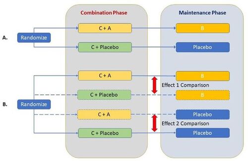
Figure 1B shows schematics of a full factorial design including treatment arms A + C and B + C, that is ideal for isolating contribution of components while adding A and B to a standard of care C. As is usual in clinical research, these designs depict A as a treatment administered together with the SOC therapy C in the combination phase, and B administered subsequently in the maintenance phase after discontinuation of C. Figure 1A depicts the general design schematics of A + B+C versus C following the real-life trials EORTC-22981/26981/NCIC-CE.3, KEYNOTE-522, and BROCADE3 noted previously.

In this article, we propose a novel tipping point analysis (TPA) using the rank preserving structural failure time (RPSFT) modeling structure that may be useful in assessing the influence of either component, A or B, on a time to event endpoint when they are administered in temporally separated treatment phases as shown in the design schematics in Figure 1A. The method is illustrated by assessing the contribution of an experimental drug, veliparib, administered during the combination phase in the BROCADE3 example. In the specific illustrative example of BROCADE3, A and B represent treatment with the same experimental drug administered in two separate phases following different dosing amounts and schedules. They are viewed as different treatments and their effects may not be assumed to be the same. In fact, the method and indices proposed in this article are general in nature and applicable irrespective of whether A and B comprise (at least in part) treatment with the same experimental therapeutic agent or not.

In subsequent sections, we describe the mathematical framework for our proposed TPA methodology in detail (section on methodology), provide published details of the study design and findings of the real-life BROCADE3 example (section on application of the proposed method), illustrate our proposed method by applying it to the example and explore estimating two different effects of interest. We then conclude by discussing the pros and cons of implementing the method and provide practical recommendations and considerations for its use.

2 Methodology

Our proposed method adopts the following common framework for analysis of a time-to-event endpoint (TTE): Let T denote the time from randomization to onset of the event of interest. In the context of clinical research, observations of such TTE variables are typically right-censored. If the censoring time is R, the observed outcome variables can be described as the right-censored TTE variable $S=$ min(T, $R)$, along with its censorship indicator $\Delta =$ I($T\le R)$, where min(.) is the minimum function and I(.) is the indicator function. We will refer to (S, $\Delta )$ as the TTE analysis doublet in this article.

Next, consider a two-arm RCT of an experimental treatment E versus a control treatment C. Let T_C, R_C, and (S_C, ${\Delta }_C)$, respectively, denote the uncensored TTE, censoring time and censored TTE analysis doublet for a subject receiving control therapy. Denote the same variables for a subject receiving the experimental therapy as T_E, R_E and (S_E, ${\Delta }_E)$. We now assume that T_C ˜F_C and T_E ˜F_E, where F_C and F_E are time to event distributions for the two treatment arms and the corresponding survival functions are denoted by S ${}_C=$ 1 –F_C and S ${}_E=$ 1 – F_E. Generally, in clinical studies, R_C and R_E are governed by independent stochastic processes independent of T_C and T_E (either unconditionally, or conditional on a set of baseline covariates), as well as the effect of the experimental treatment. When most of the censoring occurs due to administrative reasons (e.g., data cutoff for analysis), R_C and R_E are also assumed to follow a common distribution G independent of S_C and S_E. We will assume these distributions to be continuous.

2.1 Traditional Approach Using Cox Regression

The Cox proportional hazards (PH) model has been the mainstay in analyzing TTE data for as long as it has existed. It is the method of choice for drawing inference about the effect of specific factors, treatment or otherwise, that influence a TTE endpoint. Let us then consider the use of Cox regression first and outline why such an approach cannot provide satisfactory solutions for the problem at hand.

A Cox PH model fitted to all data from a trial of E (i.e., A + B+C) versus C can be written as $S_E(t)={\left[S_C(t)\right]}^{\theta }$. with θ being the hazard ratio (HR) between E and C. Let us also consider a Cox model with time-dependent covariates I_A(.) and I_B(.) that are indicators of time-periods prior to and following initiation of maintenance (with B or placebo), respectively. In its simplest form, this model can then be written as:(1) $$S_E\left(t\right)={\left[S_C\left(t\right)\right]}^{{\theta }_1{I}_A\left(t\right)+{\theta }_2{I}_B\left(t\right)}.$$(1)

To better understand what this model is estimating, suppose $S_E^A$ and $S_C^A$ denote survival functions for the experimental and control arms for the time interval between randomization and the onset of maintenance therapy or an event, whichever occurs earlier. We then have $S_E^A(u)={\left[S_C^A(u)\right]}^{{\theta }_1}$, that is, ${\theta }_1$ is the HR between the treatment arms during this interval. Similarly, we obtain $S_E^B(v)={\left[S_C^B(v)\right]}^{{\theta }_2}$ where $S_E^B$ and $S_C^B$ are survival functions for the experimental and control arms for time from onset of maintenance therapy to an event among subjects who ultimately receive maintenance therapy (with possibly different populations for the two arms), and θ₂ is the HR that emerges between these two treatment arms during the maintenance phase, conditional on the different combination-phase treatment received prior to it. Thus, if one splits the dataset into two mutually exclusive subsets where the TTE observations for all subjects who received maintenance therapy is censored at the onset of that phase and observations for subjects who only received combination therapy (i.e., C + A/matching placebo) is kept as is in the first, and only the TTE observations starting from the onset of maintenance is retained in the second (for subjects who received maintenance therapy), then simple Cox regression with treatment arm as covariate of these two subsets and the model with time-varying covariates presented in Equation (1)(1) $$S_E\left(t\right)={\left[S_C\left(t\right)\right]}^{{\theta }_1{I}_A\left(t\right)+{\theta }_2{I}_B\left(t\right)}.$$(1) would yield the same estimates of θ₁ and ${\theta }_2$, respectively.

We ask the reader now to note that, given the original study design (A + B+C versus C), it is not possible to isolate effects of the two phases using the model shown above. Any carryover effect of A emerging after the onset of maintenance is confounded with possible early effects of B and cannot be accounted for without arbitrarily assigning a washout period for the effect of A (i.e., arbitrarily extending the positive support of $I_A)$. The Cox model also cannot account for either a potentially delayed effect of B without arbitrarily shortening the positive support of I_B or potential differences in populations of subjects who transition to maintenance therapy on the two arms. As such, θ₂ does not necessarily represent the pure effect of maintenance with B. And since comparative measurement of time-to-event during the combination phase is censored in the model when subjects initiate maintenance, ${\theta }_1$ cannot assess the full treatment effect of adding A during the combination phase.

2.2 Tipping Point Analysis by Counterfactual Elicitation Using RPSFT Modeling

In causal inference of TTE endpoints in RCTs, RPSFT modeling is typically used to account for the presence of treatment switching. It provides a method for estimating and simulating counterfactual observations of the TTE under no switching ($T^{\prime })$ by modifying the actual observed TTE under switching ($T)$ through an adjustment factor λ. Let X denote the time to onset of the intercurrent event (ICE) of treatment switching from randomization. If $Y=T-X$, then one can represent the counterfactual TTE observation under no switching as:$$T^{\prime }=X+\lambda Y$$

In modeling, when interest lies in estimating $T^{\prime }$, one attempts to estimate the factor λ first and then uses it to remove the influence of the ICE from T (Robins and Tsiatis 1991; White et al. 1997; White et al. 1999; Latimer et al. 2014, 2017; Latimer, Abrams, and Siebert 2019). When the event of interest is an undesirable clinical outcome (such as progression of a disease), a positive effect of the ICE (treatment switching) would imply λ < 1 and T > T’, that is, time to the event would be delayed (or prolonged) by switching to a more efficacious treatment. Conversely, λ > 1 and T < T’ would represent a negative effect of the ICE. As a convention, for subjects who do not experience the ICE, we will set $Y=$0 and $X=T$ (the TTE). Within our proposed methodology, we will refer to this as the RPSFT structure and use it to generate counterfactual observations from hypothetical treatment arms using the observed trial data. We are not interested in the first step (Latimer et al. 2017) of estimating the factor λ invoking additional assumptions. Instead, we pair the RPSFT modeling structure with a tipping point approach to accomplish our inferential goals.

Tipping point analysis (Permutt 2016; Zhao et al. 2016) is an approach for assessing the impact of missing observations on statistically significant findings of an RCT when there is reason to suspect that those results are substantially influenced by that missingness. The approach works by imputing data for missing observations in a manner that is progressively conservative (i.e., biased against the experimental arm) until statistical significance is lost. The amount of conservatism is controlled by one or more parameters, and the parameter setting at which the imputation-based treatment difference crosses a specified threshold (e.g., becomes nonsignificant) is then referred to as the “tipping point.”

The method proposed in this article combines elements from these two techniques by first using the RPSFT structure in a natural way to account for the influence of component phases within a treatment regimen on study outcomes, and then performing a TPA using that structure to infer about the contribution of the specific treatment phase of interest. In describing our approach, we will hereafter denote by C, A + C, B + C, and A + B+C the corresponding treatments/regimens as well as study arms comprising those same treatments/regimens. The first three, C, A + C, and B + C can be considered with (for blinded RCTs) or without (for open-label RCTs) matching placebos for A and/or B.

Let us once again consider the RCT design depicted in Figure 1A where each subject’s treatment consists of a combination phase followed by a maintenance phase. On the experimental arm, treatment A is given in combination with C during the combination phase, followed by treatment B in the maintenance phase. On the control arm, patients receive C with matching placebo for A during the combination phase followed by placebo maintenance. Our inferential interest then lies in two distinct treatment effects:

• Effect 1: The contribution of A to the effect of the full regimen (A + B+C); and

• Effect 2: The sole effect of adding A to C (i.e., without the use of B in the regimen).

Effect 1 is best estimated from an RCT comparing A + B+C to B + C and Effect 2 is best estimated from an RCT comparing A + C to C (see Figure 1B). Since our actual design (Figure 1A) does not include either an A + C or a B + C arm, we will simulate counterfactual outcomes from such arms as described below.

2.2.1 Model Set-up and Assessment Method for Effect 1

For estimation of Effect 1 we propose to simulate counterfactual observations from a hypothetical treatment arm B + C by modifying observations on the original control arm C using the RPSFT structure, while leaving observations on the experimental arm A + B+C unchanged. The RPSFT model here postulates that the adjusted time to event for subjects on the hypothetical control treatment B + C may be obtained as:(2) $$T_C^{\prime }=X_C+{\lambda }_C\left(T_C-X_C\right)=X_C+{\lambda }_C{Y}_C.$$(2)

Since censorship is assumed to follow an independent distribution G, censoring times (observed or unobserved) would remain unaffected in the counterfactual. For assessing Effect 1, note that the adjustment factor λ_C only applies to control-arm subjects who actually received maintenance therapy with placebo, that is, for those with observed Y_C > 0. Observations on the experimental arm are left unaltered. When the experimental regimen A + B+C shows a benefit that is (hypothesized to be) primarily due to B, one assumes ${\lambda }_C\ge 1$.

Let $\theta ({\lambda }_C)$ denote the estimated hazard ratio (HR) between the experimental arm and the hypothetical control arm in the simulated sample; $p({\lambda }_C)$ be the one-sided p-value for the test of significance of $H_0:\theta ({\lambda }_C)\ge 1\text{versus}{H}_A:\theta ({\lambda }_C)<1$; and ${\theta }_2({\lambda }_C)$ be the estimated hazard ratio between the experimental and the hypothetical control arm for the maintenance phase (coefficient of I_B in a corresponding Cox regression). Suppose ${\theta }^{\ast }$ and ${\theta }_2^{\ast }$ are the originally observed hazard ratios between the treatment arms (overall and during the maintenance period) of the study, and $p^{*}$ be the original one-sided p-value for testing $H_A:\theta <1$. In this formulation, λ_C alone controls the counterfactual effect of the hypothetical control arm B + C and we can progressively increase it until a certain “tipping point” is reached. For our approach, we naturally require that $\theta (1)={\theta }^{\ast }<1$ and $p(1)=p^{\ast }$. We propose calculating tipping points using the following criteria:

1. A value of ${\lambda }_C\ge 1$ that leads to loss of statistical significance of the overall treatment difference between the two arms. This follows the traditional “tipping point” approach. If the corresponding tipping point is denoted ${\lambda }_{Ca}^{\ast }$, it is then defined as ${\lambda }_{Ca}^{\ast }=\text{inf}\{{\lambda }_C:p({\lambda }_C)\ge 0.025\}$. It is easy to see that $\theta ({\lambda }_{Ca}^{\ast })$ would approximately be equal to the minimum detectable difference (MDD) of the study. The higher the estimate of ${\lambda }_{Ca}^{\ast }$, the more likely it is that any statistical significance between arms of the actual study design is not solely an effect of maintenance with B.

2. A value of ${\lambda }_C\ge 1$ that “neutralizes” the treatment difference observed during the maintenance phase of the study. We define the tipping point as ${\lambda }_{Cb}^{\ast }=\text{inf}\left\{{\lambda }_C:{\theta }_2({\lambda }_C)\ge 1\right\}$. Since ${\lambda }_{Cb}^{\ast }$ “removes” the treatment difference emerging after initiation of B (that may also include some carryover effect of A), $\theta ({\lambda }_{Cb}^{\ast })$ provides an assessment of the minimum effect that can solely be ascribed to the addition of treatment A to the control C.

3. A value of ${\lambda }_C\ge 1$ that “neutralizes” the entire treatment difference between the two arms (A + B+C and C). We define this tipping point as ${\lambda }_{Cc}^{\ast }=\text{inf}\left\{{\lambda }_C:\theta ({\lambda }_C)\ge 1\right\}$. The higher the value of ${\lambda }_{Cc}^{\ast }$, especially compared to ${\lambda }_{Cb}^{\ast }$, the more likely it is that the observed treatment difference between arms of the actual study is not solely an effect of B.

All three of these tipping points provide an assessment of the contribution of the combination phase to the full regimen in distinct ways.

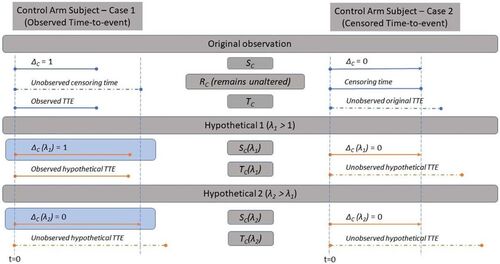
We now explain how counterfactual observations from the hypothetical experimental arm B + C shown in Figure 1B may be simulated based on the observed data for the control arm C in the original trial (Figure 1A). The following proposition formalizes that censored observations on the control arm C will remain unchanged by our proposed approach for estimating effect 1.

Proposition 1a.

For the ith subject on the control arm who receives placebo maintenance, suppose the observed TTE analysis doublet is $(s_{Ci},{\delta }_{Ci})$ and the subject’s time to initiating placebo maintenance, time to censoring and time from initiating maintenance therapy to an event (unobserved when ${\delta }_{Ci}=0)$ are $x_{Ci},r_{Ci}$ and $y_{Ci},$ respectively. Then, for any given value of ${\lambda }_C\ge 1,$ the subject’s counterfactual TTE analysis doublet $(s_{Ci}^{\prime },{\delta }_{Ci}^{\prime }),$ can be obtained as:$$\begin{array}{cc}(s_{Ci}^{\prime },{\delta }_{Ci}^{\prime })=(t_{Ci}^{\prime },1)& \text{if}{\delta }_{Ci}=1\text{and}{t}_{Ci}^{\prime }=x_{Ci}+{\lambda }_C{y}_{Ci}:\le r_{Ci};\\ =(r_{Ci},0)& \text{if}{\delta }_{Ci}=0;\text{or if}{\delta }_{Ci}=1\text{and}{t}_{Ci}^{\prime }>r_{Ci}.\end{array}$$

Proof.

Given that ${\lambda }_C\ge 1$ we find $t_{Ci}^{\prime }=x_{Ci}+{\lambda }_C{y}_{Ci}\ge x_{Ci}+y_{Ci}=t_{Ci}$.

When ${\delta }_{Ci}=0$, we get $t_{Ci}^{\prime }\ge t_{Ci}>r_{Ci}$, and one derives:$$\begin{array}{c}{\delta }_{Ci}^{\prime }=I\left(t_{Ci}^{\prime }\le r_{Ci}\right)=I\left(t_{Ci}\le r_{Ci}\right)={\delta }_{Ci}=0;\\ s_{Ci}^{\prime }=s_{Ci}=r_{Ci}\end{array}.$$

When ${\delta }_{Ci}=1,x_{Ci},y_{Ci}$ and the actual time to event $t_{Ci}=x_{Ci}+y_{Ci}$ would have been observed. Since ${\lambda }_C\ge 1$ and $t_{Ci}^{\prime }\ge t_{Ci}$, the hypothetical observation is observed if $t_{Ci}^{\prime }\le r_{Ci}$ else the observation is censored. □

Figure 2 provides a schematic elicitation of the counterfactual events generated in effect 1.

Fig. 2 Diagram representing the results shown in Proposition 1a and counterfactual elicitation for the assessment of Effect 1.

When an original observation is not censored, we propose to simulate its unobserved censoring time r_Ci conditional on the fact that $t_{Ci}\le r_{Ci}$. This conditioning fulfills the requirement that when B does not have an effect, that is, when ${\lambda }_C=1$, the original observations on C will remain unaltered and $\theta ({\lambda }_C)=\theta (1)={\theta }^{\ast }$.

There are essentially two ways of simulating r_Ci from this conditional distribution:

1. For a well-conducted study with low loss-to-follow-up rates, (where censoring mostly occurs due to data cutoff for analysis), it is reasonable to assume that the counterfactual disease progression or death of an originally uncensored subject would still have been observed if the counterfactual event were to occur by the data cutoff date. In other words, to construct the hypothetical survival doublet for analysis, r_Ci may simply be imputed using the time from randomization to the data cutoff date when it is unobserved.

2. If censoring due to reasons other than administrative ones (e.g., data cutoff) are nonnegligible, then it is better to obtain an estimate of the common, independent censorship distribution G by fitting an appropriate parametric or semiparametric survival model to the study data after reversing the censorship indicator. This reduces simulation of the censoring times to the simple task of sampling r_Ci from the fitted model using rejection sampling conditional on $r_{Ci}\ge t_{Ci}$.

Once the unobserved censoring times r_Ci have been simulated, for any given value of λ_C the counterfactual TTE analysis doublet can be generated using Proposition 1a.

2.2.2 Model Set-up and Assessment Method for Effect 2

When interest lies in Effect 2, we propose to simulate counterfactual observations from a hypothetical treatment arm A + C through modification of the real observations on the experimental arm (A + B+C), leaving observations on the control arm unchanged. In this case, the RPSFT model is set up as follows:$$T_E^{\prime }=X_E+{\lambda }_E{Y}_E.$$

Since maintenance with treatment B is believed to be efficacious, in this case one assumes $0<{\lambda }_E\le 1$. In other words, the TTE endpoint is shortened if B is replaced by placebo on the experimental arm in the maintenance phase. We can now progressively decrease the factor λ_E until a tipping point is crossed. Like before, we define our choices for the tipping point in this case as ${\lambda }_{Ea}^{\ast }=\text{sup}\left\{{\lambda }_E:p({\lambda }_E)\ge 0.025\right\}$, ${\lambda }_{Eb}^{\ast }=\text{sup}\left\{{\lambda }_E:{\theta }_2({\lambda }_E)\ge 1\right\}$ and ${\lambda }_{Ec}^{\ast }=\text{sup}\left\{{\lambda }_E:\theta ({\lambda }_E)\ge 1\right\}$. Also, all three of these tipping points provide an assessment of the contribution of the combination phase to the full regimen in distinct ways as before.

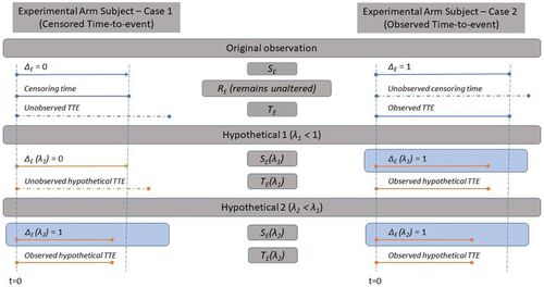
For assessing Effect 2, note that the adjustment factor ${\lambda }_E\le 1$ only applies to subjects on the experimental treatment arm, who originally received maintenance therapy with B (those with observed $Y_E>0)$. Observations on the control arm are left unaltered. Similar, to Proposition 1a, the following proposition formalizes how the TTE analysis doublet can be constructed in this case.

Proposition 1

b. For the ith subject on the experimental arm who receives maintenance with B, let the observed TTE analysis doublet be $(s_{Ei},{\delta }_{Ei})$ with time to initiating maintenance $x_{Ei},$ time to censoring r_Ei and time from initiating maintenance to an event y_Ei (possibly unobserved). Let $t_{Ei}^{\prime }=x_{Ei}+{\lambda }_E{y}_{Ei}$. Then, given any $0<{\lambda }_E\le 1,$ the counterfactual TTE analysis doublet can be obtained as:$$\begin{array}{cc}(s_{Ei}^{\prime },{\delta }_{Ei}^{\prime })=(t_{Ei}^{\prime },1)& \text{if}{\delta }_{Ei}=1;\text{or if}{\delta }_{Ei}=0\text{and}\\ & \hspace{1em}{\lambda }_E{y}_{Ei}\le r_{Ei}-x_{Ei};\\ =(r_{Ei},0)& \text{if}{\delta }_{Ei}=0\text{and}{\lambda }_E{y}_{Ei}>r_{Ei}-x_{Ei}.\end{array}$$

Proof.

Given ${\lambda }_E\le 1$, observe that $t_{Ei}^{\prime }=x_{Ei}+{\lambda }_E{y}_{Ei}\le x_{Ei}+y_{Ei}=t_{Ei}$ and, since $t_{Ei}^{\prime }\le t_{Ei}\le r_{Ei}$ for ${\delta }_{Ei}=1,$ we have $(s_{Ei}^{\prime },{\delta }_{Ei}^{\prime })=(t_{Ei}^{\prime },1)$. On the other hand, when ${\delta }_{Ei}=0$, r_Ei is observed but t_Ei is censored (and one must impute $y_{Ei})$. If ${\lambda }_E{y}_{Ei}\le r_{Ei}-x_{Ei}$, then $t_{Ei}^{\prime }\le r_{Ei}$ and the counterfactual TTE would also be observed, i.e., ${\delta }_{Ei}^{\prime }=1$. Otherwise, if ${\lambda }_E{y}_{Ei}>r_{Ei}-x_{Ei}$ then $t_{Ei}^{\prime }>r_{Ei}$ and it remains censored, that is, ${\delta }_{Ei}^{\prime }=0$, with $s_{Ei}^{\prime }=r_{Ei}$. □

Figure 3 provides a schematic elicitation of the counterfactual events generated in effect 2.

Fig. 3 Diagram representing the results shown in Proposition 1b and counterfactual elicitation for the assessment of Effect 2.

Unobserved event times t_Ei for subjects who receive maintenance with B and are censored need to be simulated conditional on $t_{Ei}>r_{Ei}$ to obtain their counterfactual observation on a hypothetical A + C arm. We can try to use an estimate of F ${}_{\mathbf{E}}$ conditional on $T_E>R_E$ to impute the time to event if it is mathematically tractable. For example, if F ${}_{\mathbf{E}}$ is an exponential distribution, then conditional on $T_E>R_E$ the distribution of T_E remains the same due to its memoryless property. Our preferred approach, however, is to use a fitted survival model to time on maintenance with B and impute $T_E^{\prime }$ conditional on $T_E>R_E$ using a rejection sampling scheme.

As the title of this section suggests, we refer to this new methodology as Tipping Point Analysis by Counterfactual Elicitation (TPACE). Interpretation of a tipping point depends on its extremeness. The more extreme the tipping point is in terms of bias against the experimental therapy, the more unlikely it is that any effect ascribed to that therapy could potentially be a result of unobserved outcomes. This assessment is usually qualitative since there is typically no clear benchmark to determine how extreme a tipping point truly is. In the next section, however, we describe how an informal interpretation of estimated Effects 1 and 2 may be obtained by calculating a contribution index involving the estimated tipping points obtained via TPACE.

2.2.2.1 Interpretating TPACE-Based Estimates and Assessing Contribution of a Treatment Phase

Given A + B+C is observed to be more effective than C, we have assumed that there exists a constant scaling λ_C (>1) of the control arm C that neutralizes the treatment difference emerging during the maintenance period of the original study following the RPSFT structure in the context of assessing Effect 1 using TPACE. Using notation introduced in the methodology section, we can denote this as $S_E^B(v)={\left[S_C^B(v)\right]}^{{\theta }_2}\cong S_C^B\left(\frac{v}{{\lambda }_C}\right)$. When $S_E^B$ follows an exponential distribution, we would surmise that ${\lambda }_C=\frac{1}{{\theta }_2}$ and $S_E^B(v)=S_C^B(v{\theta }_2)$.

If the observed TTE duration following initiation of maintenance therapy on the original control arm C is prolonged using the scaling factor $\frac{1}{{\theta }_2}$ (without concern for potential additional censoring when TTE is prolonged) and ${\theta }^{\prime }$ denotes the resultant HR, then we can derive the relationship between S_E and S_C as:$$S_E\left(t\right)\cong {\left[S_C\left(x_C+\frac{t-x_C}{{\theta }_2}\right)\right]}^{{\theta }^{\prime }}.$$

Considering the time dilation shown above to be one way of neutralizing the effect of the maintenance phase θ₂ by reducing it to nearly 1, one may view ${\theta }^{\prime }$ as providing an assessment of the residual effect that can only be ascribed to the addition of A during the combination phase. As one might expect, this results in a value of ${\theta }^{\prime }$ approximately equal to θ₁. To realize this through counterfactuals one simply scales both event and censoring times during the maintenance phase by the same factor representing a treatment effect and rerunning the Cox model. However, it distorts the censoring distribution such that it is no longer independent of the TTE distribution and treatment effect, and therefore violates fundamental assumptions of the Cox model. In practice, when censoring occurs primarily due to length of follow-up, the above scaling is tantamount to selectively increasing the follow-up period for subjects initiating maintenance and in a manner that is dependent on the treatment effect. Hence, findings thereof are biased.

2.2.3 Assessment Index for Effect 1

In TPACE we use proper counterfactual observations to avoid the distortion of the censorship distribution mentioned above and neutralize the effect of the component phases within the Cox model using the RPSFT structure. Thus, for Effect 1 we estimate the scaling factor ${\lambda }_{Cb}^{\ast }>1$ that yields a counterfactual ${\theta }_2({\lambda }_{Cb}^{\ast })\cong 1$ and the scaling factor ${\lambda }_{Cc}^{\ast }$ such that we have counterfactual $\theta ({\lambda }_{Cc}^{\ast })\cong 1$ using TPACE, while keeping the censoring distribution nearly unchanged (and independent). If now $T_C^E$ and $T_C^B$, respectively, denote the estimates of the prolonged hypothetical TTE on the control arm that neutralize the overall difference between arms of the actual study (mimicking arm A + B+C) and the difference between treatment arms that emerged after onset of maintenance (mimicking arm B + C), we may write them as:(3) $$T_C^E=X_C+{\lambda }_{Cc}^{\ast }{Y}_C\text{and}{T}_C^B=X_C+{\lambda }_{Cb}^{\ast }{Y}_C.$$(3)

We can then split the total estimated delay in TTE on the experimental arm (E = A+B + C) gained over C as the sum of the estimated delay gained after onset of maintenance $T_C^B-T_C$ and the delay gained prior to that (credited to treatment A when added on to C), denoted $T_C^A$, that is,$$T_C^E-T_C=\left(T_C^E-T_C^B\right)+\left(T_C^B-T_C\right)=T_C^A+\left(T_C^B-T_C\right).$$

We thus obtain:$$\mathit{Estimated}\mathrm{}\mathit{time}\mathrm{}\mathit{gained}\mathrm{}\mathit{with}\mathrm{}E\mathrm{}\text{over}\mathrm{}\mathrm{C}=T_C^E-T_C=({\lambda }_{Cc}^{\ast }-1)Y_C,$$$$\text{Time}\mathrm{}\text{gained}\mathrm{}\text{following}\mathrm{}\text{onset}\mathrm{}\text{of}\mathrm{}\mathrm{B}=T_C^B-T_C=({\lambda }_{Cb}^{\ast }-1)Y_C$$, and $$\text{Time}\mathrm{}\text{gained}\mathrm{}\text{due}\mathrm{}\text{to}\mathrm{}\text{adding}\text{A}\text{in}\mathrm{}\mathrm{A}+\mathrm{B}+\mathrm{C}=T_C^A=(T_C^E-T_C^B)=({\lambda }_{Cc}^{\ast }-{\lambda }_{Cb}^{\ast })Y_C.$$

We may now use the above expressions to derive the contribution index of A to the overall effect of E (i.e., A + B+C versus B + C) as(4) $$C_C^A=\frac{\left(T_C^E-T_C^B\right)}{\left(T_C^E-T_C\right)}=\frac{\left({\lambda }_{Cc}^{\ast }-{\lambda }_{Cb}^{\ast }\right)}{\left({\lambda }_{Cc}^{\ast }-1\right)}.$$(4)

And the contribution index of B to overall effect of E is then the complement of $C_C^A$ derived as$$C_C^B=\frac{\left(T_C^B-T_C\right)}{\left(T_C^E-T_C\right)}=\frac{\left({\lambda }_{Cb}^{\ast }-1\right)}{\left({\lambda }_{Cc}^{\ast }-1\right)}=1-C_C^A.$$

Since the basic Cox model used in effect-neutralization does not account for effects of A carried over to the maintenance phase, $C_C^A$ should be viewed as an index of minimum contribution of A and $C_C^B$ as an index of maximum contribution of B to the total time gained by E over C.

2.2.4 Assessment Index for Effect 2

When using TPACE for Effect 2, we estimate the scaling factor ${\lambda }_{Eb}^{\ast }<1$ such that counterfactual ${\theta }_2({\lambda }_{Eb}^{\ast })\cong 1$ and the scaling factor ${\lambda }_{Ec}^{\ast }<1$ such that counterfactual $\theta ({\lambda }_{Ec}^{\ast })\cong 1$, maintaining independence of the censoring distribution. If now $T_E^E$ and $T_E^B$, respectively, denote the estimates of the shortened hypothetical TTE on the experimental arm that eliminates the overall difference between arms E and C (thus mimicking arm C) and the difference between treatment arms that emerged after onset of maintenance (thus mimicking arm A + C), we may write them as:$$T_E^E=X_E+{\lambda }_{Ec}^{\ast }{Y}_E\text{and}{T}_E^B=X_E+{\lambda }_{Eb}^{\ast }{Y}_E.$$

The difference between the two, $T_E^B-T_E^E$ then yields an estimate of the gain due to adding A alone to C (i.e., Effect 2) on the time scale. Likewise, we can then obtain:$$\text{Estimated}\mathrm{}\text{time}\mathrm{}\text{gain}\mathrm{}\text{of}\text{E}\text{over}\text{C}\left(\text{that}\mathrm{}\text{was}\mathrm{}\text{eliminated}\right)=T_E-T_E^E=(1-{\lambda }_{Ec}^{\ast })Y_E,\mathrm{}\text{and}$$$$\text{estimated}\mathrm{}\text{time}\mathrm{}\text{gain}\mathrm{}\text{following}\mathrm{}\text{onset}\mathrm{}\text{of}\text{B}\left(\text{that}\mathrm{}\text{was}\mathrm{}\text{eliminated}\right)=T_E-T_E^B=(1-{\lambda }_{Eb}^{\ast })Y_E.$$$$\text{Therefore},\mathrm{}\text{estimated}\mathrm{}\text{time}\mathrm{}\text{gain}\mathrm{}\text{only}\mathrm{}\text{due}\mathrm{}\text{to}\text{A}\text{in}\mathrm{}\mathrm{A}+\mathrm{C}=T_E^A=\left(T_E^B-T_E^E\right)=\left({\lambda }_{Eb}^{\ast }-{\lambda }_{Ec}^{\ast }\right)Y_E.$$

We now derive the minimum individual efficacy index of A as$$E_E^A=\frac{\left(T_E^B-T_E^E\right)}{\left(T_E-T_E^E\right)}=\frac{\left({\lambda }_{Eb}^{\ast }-{\lambda }_{Ec}^{\ast }\right)}{\left(1-{\lambda }_{Ec}^{\ast }\right)}.$$

And similarly derive the estimated maximum index of contribution of B to the full benefit of E when B is added to A + C by $E_E^B=1-E_E^A$.

2.2.5 Statistical Inference for TPACE-Based Assessment Indices

We provide next an approach for calculating confidence intervals of the assessment indices proposed above. While the clinical meaningfulness of the estimate of an index depends on the context of application, its confidence interval (CI) provides an inferential framework for decision making when some consensus can be reached about the range of percentage values for it that may be considered clinically relevant. For example, if a minimally clinically relevant percentage contribution threshold of A can be agreed upon, one can conclude that the contribution of A to A + B+C is clinically meaningful and statistically significant if the lower limit of the CI of $C_C^A$ exceeds that threshold.

Let us first describe the approach for obtaining a CI of $C_C^A$. We begin by noting that, per Equation (4)(4) $$C_C^A=\frac{\left(T_C^E-T_C^B\right)}{\left(T_C^E-T_C\right)}=\frac{\left({\lambda }_{Cc}^{\ast }-{\lambda }_{Cb}^{\ast }\right)}{\left({\lambda }_{Cc}^{\ast }-1\right)}.$$(4) , $C_C^A$ is a function of (the scaling factors) ${\lambda }_{Cb}^{\ast }$ and ${\lambda }_{Cc}^{\ast }$, that in turn are derived from the following equations:$$\text{For}{\lambda }_{Cc}^{\ast }:\theta \left({\lambda }_{Cc}^{\ast }\right)=1\text{and}\mathrm{}\theta \left(1\right)={\theta }^{\ast }$$$$\text{For}\mathrm{}{\lambda }_{Cb}^{\ast }:{\theta }_2\left({\lambda }_{Cb}^{\ast }\right)=1\text{and}{\theta }_2\left(1\right)={\theta }_2^{\ast }.$$

As these equations indicate, uncertainty in estimating $C_C^A$ stems from variability in estimating ${\theta }^{\ast }$ and ${\theta }_2^{\ast }$, and the distribution of $C_C^A$ is induced by the joint distribution of ${\theta }^{\ast }$ and ${\theta }_2^{\ast }$. The relationships between λ and θ-s are however analytically intractable, which prevents derivation of a CI for $C_C^A$ directly. We will therefore adopt a fiducial approach.

Consistent with our basic model setup for assessing Effect 1 and Equation (2)(2) $$T_C^{\prime }=X_C+{\lambda }_C\left(T_C-X_C\right)=X_C+{\lambda }_C{Y}_C.$$(2) , we condition our derivation on holding the TTE on the experimental arm ($T_E)$ and the observations prior to transitioning to placebo maintenance from the control arm ($X_C)$ fixed. Recall from Equation (3)(3) $$T_C^E=X_C+{\lambda }_{Cc}^{\ast }{Y}_C\text{and}{T}_C^B=X_C+{\lambda }_{Cb}^{\ast }{Y}_C.$$(3) that $T_C^E$ and $T_C^B$ are the TTE variables that neutralize the observed overall effect ${\theta }^{\ast }$ and the observed maintenance phase effect ${\theta }_2^{\ast }$, respectively. Let $\left[{\theta }_{2L}^{\ast },{\theta }_{2U}^{\ast }\right]$ denote a confidence interval of ${\theta }_2^{\ast }$. For example, one can be obtained by fitting the Cox model in Equation (1)(1) $$S_E\left(t\right)={\left[S_C\left(t\right)\right]}^{{\theta }_1{I}_A\left(t\right)+{\theta }_2{I}_B\left(t\right)}.$$(1) . Let us now consider its lower confidence limit (LCL) ${\theta }_{2L}^{\ast }$ and use it to derive a LCL for $C_C^A$. We note here that the LCL of $C_C^A$ is inferentially more important than its upper confidence limit (UCL).

Let ${\theta }_2({\lambda }_{CL}^{\ast })={\theta }_{2L}^{\ast }$ and ${\theta }_2({\lambda }_{CU}^{\ast })={\theta }_{2U}^{\ast }$. Since the functions $\theta (·)$ and ${\theta }_2(·)$ define monotonically increasing, 1–1 and continuous mappings in the context of Effect 1 when the underlying TTE distributions are continuous, the inverses of these functions exist, and the above expressions uniquely define ${\lambda }_{CL}^{\ast }$ and ${\lambda }_{CU}^{\ast }$. Let us now consider the TTE variable on the control arm corresponding to ${\lambda }_{CL}^{\ast }$, namely $T_{CL}=X_C+{\lambda }_{CL}^{\ast }{Y}_C=X_C+Y_{CL}$ (instead of $T_C=X_C+Y_C)$ as the starting point for our approach to effect neutralization (overall and for B), similar to how $C_C^A$ was constructed. Heuristically, we can then argue that, starting with the ${\theta }_{2L}^{\ast }$ (a larger effect of B):

Estimated time gained with E over $C=T_C^E-T_{CL}=({\lambda }_{Cc}^{\ast }-{\lambda }_{CL}^{\ast })Y_C$.

And, since the estimated time gained due to A remains $T_C^A=(T_C^E-T_C^B)=({\lambda }_{Cc}^{\ast }-{\lambda }_{Cb}^{\ast })Y_C$, one obtains a LCL of $C_C^A$ by(5) $$c_{CL}^A=\frac{\left({\lambda }_{Cc}^{\ast }-{\lambda }_{Cb}^{\ast }\right)}{\left({\lambda }_{Cc}^{\ast }-{\lambda }_{CL}^{\ast }\right)}.$$(5)

However, since both $\theta (\lambda )$ and ${\theta }_2(\lambda )$ are functions of the same argument λ, and hence, vary together, we need to further formalize this argument. For this, given that Arm E (A + B+C) observations, and hence, T_E remains unchanged in assessing Effect 1, we find that $\theta ({\lambda }_{CL}^{\ast })={\theta }_L^{\ast \ast }$ is the overall hazard ratio of E over C corresponding to ${\theta }_{2L}^{\ast }$, that is, it is the hazard ratio obtained when T_E is compared with T_CL. We caution the reader here not to interpret ${\theta }_L^{\ast \ast }$ as a LCL of ${\theta }^{\ast }$.

We now try to answer the following two questions: If ${\theta }_{2L}^{\ast }$ was the observed hazard ratio for the maintenance phase instead of ${\theta }_2^{\ast }$, then what would be the scaling factor ($\lambda )$ values that will inflate Y_CL (the new TTE from onset of maintenance on C) such that a) the maintenance phase effect ${\theta }_{2L}^{\ast }$ is neutralized, and b) the corresponding overall effect ${\theta }_L^{\ast \ast }$ is neutralized?

To answer these questions, we rewrite:$$\begin{array}{c}{T}_C^E=X_C+{\lambda }_{Cc}^{\ast }{Y}_C=X_C+\frac{{\lambda }_{Cc}^{\ast }}{{\lambda }_{CL}^{\ast }}{Y}_{CL};\\ T_C^B=X_C+{\lambda }_{Cb}^{\ast }{Y}_C=X_C+\frac{{\lambda }_{Cb}^{\ast }}{{\lambda }_{CL}^{\ast }}{Y}_{CL}.\end{array}$$

Now using Equation (4)(4) $$C_C^A=\frac{\left(T_C^E-T_C^B\right)}{\left(T_C^E-T_C\right)}=\frac{\left({\lambda }_{Cc}^{\ast }-{\lambda }_{Cb}^{\ast }\right)}{\left({\lambda }_{Cc}^{\ast }-1\right)}.$$(4) with ${\lambda }_{Cc}^{\ast \ast }=\frac{{\lambda }_{Cc}^{\ast }}{{\lambda }_{CL}^{\ast }}$ and ${\lambda }_{\mathit{CbU}}^{\ast }=\frac{{\lambda }_{Cb}^{\ast }}{{\lambda }_{CL}^{\ast }}$ once again yields expression (5) above for a LCL of $C_C^A$. An UCL of $C_C^A$ can be obtained similarly. Thus, our proposed CI $\left[c_{CL}^A,c_{CU}^A\right]$ for $C_C^A$ can be calculated as(6) $$c_{CL}^A=\frac{\left({\lambda }_{Cc}^{\ast }-{\lambda }_{Cb}^{\ast }\right)}{\left({\lambda }_{Cc}^{\ast }-{\lambda }_{CL}^{\ast }\right)}\text{and}{c}_{CU}^A=\frac{\left({\lambda }_{Cc}^{\ast }-{\lambda }_{Cb}^{\ast }\right)}{\left({\lambda }_{Cc}^{\ast }-{\lambda }_{CU}^{\ast }\right)}.$$(6)

And one can also think of $\left[{\lambda }_{\mathit{CbL}}^{\ast }=\frac{{\lambda }_{Cb}^{\ast }}{{\lambda }_{CU}^{\ast }},{\lambda }_{\mathit{CbU}}^{\ast }=\frac{{\lambda }_{Cb}^{\ast }}{{\lambda }_{CL}^{\ast }}\right]$ as a confidence interval of λ_Cb.

Now, in terms of statistical inference, if $c^{\ast }>0$ is the smallest percentage contribution that one will consider to be clinically meaningful, then one can conclude that the contribution of A is clinically meaningful and statistically significant if $c_{CL}^A\ge c^{\ast }$.

In the case of Effect 2, one can similarly calculate a CI of $E_E^A$ and draw statistical inferences in a similar manner. We will skip the details here for brevity and to avoid introducing additional notations. We would however like to remind readers that, in the context of Effect 2 (Arm A + C versus Arm C), the mappings $\theta (·)$ and ${\theta }_2(·)$ are monotonically decreasing one-to-one functions of the argument λ (which mostly is a shrinkage factor in this case) and are different from functions denoted by same notations in the context of Effect 1. As such, they need to be interpreted accordingly. We also note that the decision threshold for $E_E^A$ can be set to 0, and if the LCL of $E_E^A$ exceeds 0, one may attempt to conclude that the effect of adding only A to C (i.e., A + C) over C, as a percentage of the overall effect of A + B+C over C, is statistically significant. While this is technically alright, it is not the same as (and hence not a substitute for) establishing a statistically significant treatment effect of A + C over C through a properly conducted RCT.

2.2.6 Counterfactual Elicitation and Bias Correction

In describing our methodology above, we have assumed that both θ and θ₂ can be estimated in a reasonably unbiased manner based on the original study observations. In the basic setup for describing our approach we have also assumed the absence of any informative censoring. We however acknowledge that this is not a given in many instances and one may have to adopt additional bias correction methods as necessary in conjunction with and prior to applying our method.

It is also easy to see that our method itself would not introduce any bias beyond any model misspecification during Cox regression or use of RPSFT. In estimating Effect 1, we generate observations for B + C based on Arm C and prolonging time in maintenance for subjects who received C (+ placebo) and transitioned to placebo maintenance. Note that these would be the same subjects who would have transitioned from C (+ placebo) to maintenance B had that been the treatment policy instead. Hence, there is no selection bias introduced in the process of counterfactual elicitation when inflating the time after initiation of placebo maintenance. Similarly, in estimating Effect 2, we shrink the time on maintenance B using observations on treatment E. Here again, no selection bias is introduced since subjects who received B would have transitioned to placebo maintenance if that had been the treatment policy (provided the A + B+C arm was still included in the study).

We would now like to point out a fundamental difference between the context of application for our method and the context of treatment switching where a hypothetical strategy or principal stratum strategy (as described in International Conference on Harmonisation E9(R1) 2020) may be used for bias correction. In the usual context of bias-correction in an RCT of E versus C using the latter approaches, a set of patients on C would typically switch over to receive E (or another drug in the same class as E) prior to observation of the event of interest, thus causing issues with a treatment policy approach (often also referred to as the ITT approach) in adequately estimating and characterizing the effect of E versus C, the principal estimand. A hypothetical or principal stratum strategy is then used to generate bias-corrected estimates of the same effect (E versus C) that can either provide sensitivities to the treatment policy based primary estimator or in some cases even replace it. In the case of a principal stratum approach only the population attribute of the primary estimand changes.

The goal of our method on the other hand, is to estimate two very different effects – Effect 1: E = A+B + C versus B + C, and Effect 2: A + C versus C from the study’s primary estimand E versus C. Thus, in the parlance of the estimand framework, we change the treatment attribute while keeping the population attribute the same (the ITT population). Also, while the RPSFT modeling structure has traditionally been used in implementing a hypothetical strategy in the context of treatment switching, the RPSFT model is used within our proposed approach in a fairly novel way. We have used it to generate counterfactuals (as a function of $\lambda )$ from treatment policies B + C and A + C that could have been studied in the original RCT to assess contribution of components but weren’t. Specifically, our method is not meant to replace any of the studied arms, E or C, for reestimating the primary estimand E versus C. We assume that reliable estimates of this effect (E versus C) are available and embark on exploring what the contribution or effect of components A (or B) could have been. If there is bias in estimating E versus C, then an appropriate bias-correction approach can be used in conjunction with our method, as Step 1 in a 2-step procedure.

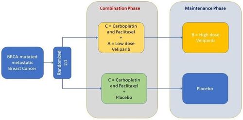
3 Application of TPACE

The methodology proposed in this article is now applied to a phase 3 randomized, double-blinded, placebo-controlled study of veliparib, an inhibitor of the enzyme poly ADP ribose polymerase (PARP), in subjects with BRCA-mutated HER2-negative breast cancer, BROCADE3 (Diéras et al. 2020). In this RCT, subjects were randomized 2:1 to receive either veliparib or placebo added on to SOC chemotherapy (CT) with carboplatin and paclitaxel (Figure 4). While treatment with all three drugs (carboplatin, paclitaxel and veliparib/placebo) could continue until disease progression or unacceptable toxicity, study subjects had the option to discontinue any of these drugs at any time. When both SOC CT drugs were discontinued without disease progression or death, subjects also had the option to receive maintenance therapy with blinded study drug, veliparib at a higher dose or placebo.

Fig. 4 BROCADE3 Study Design.

The study showed a statistically significant improvement in progression-free survival (PFS) between the two treatment arms (Table 1, Figure 5). Subjects across both arms received 7.5 months of SOC CT on average (median 6.3 months) with 37% receiving veliparib monotherapy maintenance at a higher dose. A total of 349 subjects had experienced at least one PFS event by the time of the primary analysis and hence, the minimum detectable difference (MDD) at the 2-sided 5% level of significance can be easily calculated to be HR approximately equal to 0.8.

Fig. 5 Progression-free survival results of the BROCADE3 study (reprinted with permission of Elsevier Pvt. Ltd. from article by Diéras et al. 2020).

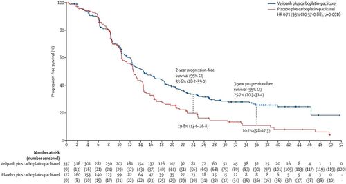
Table 1 Summary of progression-free survival results of study BROCADE3.

	Experimental Arm (n = 337)	Control Arm (n = 172)
PFS events	217	132
Censored observations	120	40
Median PFS (months)	14.5	12.6
Hazard ratio (95% CI)${}_{\#}^{\ast }$	0.71 (0.57, 0.88)
Log-rank ${}_{\ast }$ p-value	0.0016

* Hazard ratio estimated by fitting Cox proportional hazard (PH) model to the data.

# Stratified by randomization stratification factors.

Generated with permission of Elsevier Private Ltd., based on data provided in Figures 2 and 3 of the article by Diéras et al. (2020)

It is important to assess the contribution of the combination phase to the overall treatment benefit of the veliparib regimen in BROCADE3 for several reasons. First, as noted in Diéras et al. (2020), the average duration of the combination phase was approximately 10 months and the survival distributions (KM curves) of the two treatment arms did not begin to separate meaningfully until approximately 12 months from randomization. However, subjects could receive combination therapy as long as it remained tolerable or until a PFS event occurred. Substantial proportions of subjects continued their combination therapy well past 12 months suggesting that the benefit of the experimental regimen may not be driven by maintenance alone. At the time of the primary analysis, as noted in Diéras et al. (2020), 38% of the 509 subjects included in the intent-to-treat (ITT) analysis had transitioned to veliparib/placebo maintenance. Second, while studies of other PARP-inhibitors as maintenance therapy alone have demonstrated substantial efficacy leading to skepticism about the utility of veliparib in the combination phase, such cross-study comparisons are inferentially fraught since studies of other PARP inhibitors were restricted only to subjects who had already received and responded to SOC CT prior to enrollment. Finally, while one cannot deem combination phase veliparib unnecessary for efficacy simply based on the above considerations, SOC CT is not without toxicity and adding veliparib to the combination phase further increases the treatment burden for study subjects.

To assess the contribution of combination-phase veliparib to the overall treatment effect, Diéras et al. (2020) published results of a Cox regression analysis of the PFS endpoint including a time-varying covariate for initiation of veliparib/placebo maintenance, treatment assigned at randomization and their interaction (Table 2). The fitted model produced HR estimates for the combination phase effect θ₁, 0.811 (95% CI: 0.622, 1.056), and the maintenance phase effect ${\theta }_2$, 0.493 (95% CI: 0.334, 0.728) favoring the veliparib arm.

Table 2 Summary of Cox proportional hazards regression of progression-free survival with time-varying covariate indicating treatment phase.

	Combination		Monotherapy
	phase Veliparib + C/P	Placebo + C/P	phase Veliparib + C/P	Placebo + C/P
Patients at risk at
beginning of phase	337	172	131	57
Events (%)	149 (44%)	88 (51%)	68 (52%)	44 (77%)
Hazard Ratio (95% CI)	0.81 (0.62, 1.06)		0.49 (0.33, 0.73)

Treatment phase was included as a time-varying covariate which was set to 1 at and after initiation of monotherapy, and to 0 prior to it.

Reprinted with permission of Elsevier Private Ltd. from article by Diéras et al. (2020).

As described earlier, we view our motivating example of BROCADE3 as a study of A + B+C versus C where C represents the SOC CT with paclitaxel and carboplatin, A is veliparib used as part of a combination phase with CT and B is veliparib monotherapy given at a higher dose during a maintenance phase after CT is discontinued (Figures 1 and 4).

3.1 Effect 1: Index of Contribution of A

We will now calculate the contribution index of A in our example using TPACE. Since the experimental regimen is more efficacious, a lower percentage of events was observed on the experimental arm compared to the control arm during the maintenance phase (Figure 5, Table 2). Among all censored observations across both arms, PFS times for most subjects (64.5%) were censored at data cutoff. We therefore simulated the counterfactual observations to assess Effect 1 by simply imputing the time from randomization to data cutoff as the unobserved censoring time for subjects who progressed or died after transitioning to maintenance monotherapy. We then calculated the tipping points for PFS following criteria (a), (b), and (c) of our methodology (Figure 6, Table 3). The respective Kaplan Meier survival probability plots are presented in Figure 7A–C.

Fig. 6 Plots of counterfactual θ₂ and θ against values of λ_C (for Effect 1) and λ_E (for Effect 2) showing tipping points for each tipping criterion using RPSFT modeling.

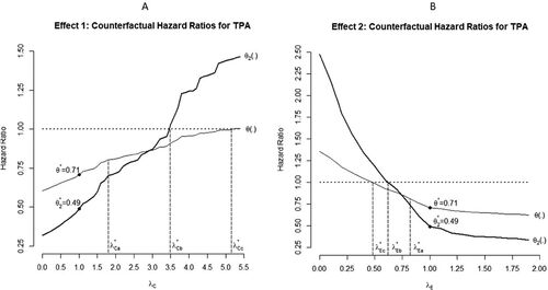
Fig. 7 Kaplan Meier plots by treatment arm at tipping points for each tipping criterion for Effect 1 (A, B, and C) and Effect 2 (D, E, and F).

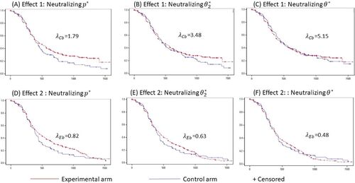
Table 3 Results of tipping point analysis evaluating effect of the combination phase.

Effect /Estimated tipping parameter	Adjustment factor at tipping point	Average No. of of Events	Hazard ratio at tipping point	P-value at tipping point
Assessment for Effect 1
${\lambda }_{Ca}^{\ast }$	1.79	342	0.802^a	0.0503${}^{\#}$
${\lambda }_{Cb}^{\ast }$	3.48	335	0.908
${\lambda }_{Cc}^{\ast }$	5.15	328	1.000
Assessment of Effect 2
${\lambda }_{Ea}^{\ast }$	0.82	379	0.811^a	0.0536${}^{\#}$
${\lambda }_{Eb}^{\ast }$	0.63	397	0.913
${\lambda }_{Ec}^{\ast }$	0..48	406	1.001

# The tipping value ${\lambda }_{Ca}^{\ast }$ and ${\lambda }_{Ea}^{\ast }$ are determined at the corresponding tipping values achieving minimum $p\mathrm{>}0.05$ (2-sided).

The estimated loss of significance tipping point ${\lambda }_{Ca}^{\ast }=1.79$ yields a “residual” counterfactual hazard ratio $\theta (1.79)=0.802$. While the similarity of this HR to the MDD (0.805) is expected, we believe its proximity to the Cox model’s estimate of ${\theta }_1=0.811$ in our example is simply coincidental. The tipping point ${\lambda }_{Cb}^{\ast }$ is estimated to be 3.48 where the counterfactual treatment differences reduce to $\theta (3.48)=0.908$ overall and ${\theta }_2(3.48)=1$ in the period following initiation of maintenance. An estimated ${\lambda }_{Cc}^{\ast }=5.15$ fully neutralizes the full, overall difference between treatment arms with counterfactual $\theta (5.15)=1$.

Expressed in words, PFS following initiation of maintenance on the control arm needs to be extended by an additional (3.48–1)*100% = 248% to get the hazard during this phase to match (on average) the hazard of the maintenance phase on the experiment arm. Since it needs to be extended by an unrealistic (5.15–1)*100% = 415% to get the PFS for the control arm to match (on average) the experimental arm overall, the contribution index of A to the overall effect of E is calculated to be:$$C_C^A=\frac{\left(5.15-3.48\right)}{\left(5.15-1\right)}=\frac{1.67}{4.15}=0.402.$$

This therefore suggests that, at least an estimated 40% of the total delay in time to disease progression or death observed on the experimental arm compared to control may be ascribed to the use of veliparib during the combination phase, and no more than 60% of the PFS prolongation after initiation of maintenance may be ascribed to maintenance veliparib alone.

The confidence interval of $C_C^A$ is calculated as (33.4%, 52.4%) based on the estimates of θ₂, 0.493 (95% CI: 0.334, 0.728). From the lower and upper confidence limits of θ₂ we obtain ${\lambda }_{CL}^{\ast }=0.145$ and ${\lambda }_{CU}^{\ast }=1.96$, and use Equation (6)(6) $$c_{CL}^A=\frac{\left({\lambda }_{Cc}^{\ast }-{\lambda }_{Cb}^{\ast }\right)}{\left({\lambda }_{Cc}^{\ast }-{\lambda }_{CL}^{\ast }\right)}\text{and}{c}_{CU}^A=\frac{\left({\lambda }_{Cc}^{\ast }-{\lambda }_{Cb}^{\ast }\right)}{\left({\lambda }_{Cc}^{\ast }-{\lambda }_{CU}^{\ast }\right)}.$$(6) to calculate (see Table 4).$$\begin{array}{c}{c}_{CL}^A=\frac{\left(5.15-3.48\right)}{\left(5.15-0.145\right)}=0.334\hspace{1em}\text{and}\\ c_{CL}^A=\frac{\left(5.15-3.48\right)}{\left(5.15-1.96\right)}=0.524.\end{array}$$

Table 4 Point estimates and 95% confidence interval of the scaling factor λ and assessment indices for Effect 1 and Effect 2.

Effect	Scaling factors		Assessment Index
Effect 1	${\lambda }_{Cc}^{\ast }$	${\lambda }_{Cb}^{\ast }$	$C_C^A$
A + B+C versus B + C	5.15 (2.63, 35.52)	3.48 (1.78, 24)	40% (33.4%, 52.4%)
Effect 2	${\lambda }_{Ec}^{\ast }$	${\lambda }_{Eb}^{\ast }$	$E_E^A$
A + C versus C	0.48 (0.25, 0.56)	0.63 (0.33, 0.73)	29% (10.4%, 39.5%)

Point estimates and 95% Confidence interval of the scaling factors and assessment indices are based on the point estimate and 95% CI of θ₂: 0.493 (95% CI: 0.334, 0.728) (See Table 2).

We also obtain a confidence interval for ${\lambda }_{Cb}^{\ast }$ as$$\left[{\lambda }_{\mathit{CbL}}^{\ast }=\frac{{\lambda }_{Cb}^{\ast }}{{\lambda }_{CU}^{\ast }}=\frac{3.48}{1.96}=1.78,{\lambda }_{\mathit{CbU}}^{\ast }=\frac{{\lambda }_{Cb}^{\ast }}{{\lambda }_{CL}^{\ast }}=\frac{3.48}{0.145}=24\right].$$

And for ${\lambda }_{Cc}^{\ast }$ as$$\left[{\lambda }_{\mathit{CbL}}^{\ast }=\frac{{\lambda }_{Cc}^{\ast }}{{\lambda }_{CU}^{\ast }}=\frac{5.15}{1.96}=2.63,{\lambda }_{\mathit{CbU}}^{\ast }=\frac{{\lambda }_{Cc}^{\ast }}{{\lambda }_{CL}^{\ast }}=\frac{5.15}{0.145}=35.52\right].$$

3.2 Effect 2: Index for the Individual Efficacy of A

As described in our methodology section, TPACE for assessing Effect 2 was performed with the shrinkage factor λ_E ($0<{\lambda }_E<1)$ applied only to those who transitioned to maintenance on the experimental arm. Counterfactual PFS times for subjects who were randomized to the experimental arm and went on to receive maintenance veliparib needed to be simulated conditional on observed data in this case. We assumed and fit an exponential distribution for the subjects’ time from initiation of maintenance to progression or death. For subjects censored during the maintenance phase, the unobserved time from censoring to potential progression or death would also follow the same exponential distribution by virtue of the lack-of-memory property of the latter. For these subjects, we therefore simulated the unobserved time from censorship to event using the fitted exponential model and added that time to the observed s_Ei to obtain t_Ei. With the time to event (t_Ei values) thus obtained for all subjects on the experimental arm, we shrank them by the factor λ_E following the rules described in the section on methodology. For subjects who were originally censored during monotherapy, if the shrunk, imputed time to event was smaller than the observed censoring time, the counterfactual observation for that subject would be an imputed event with PFS time set equal to the imputed time to event. Otherwise, the original censored TTE observation was left unchanged. Once again, starting from ${\lambda }_E=1$ (where results are same as that of the primary analysis), grid-searches by decreasing the value of λ_E were performed to find tipping points corresponding to thresholds (a), (b) and (c) for PFS (Figure 6, Table 3). The respective Kaplan Meier survival probability plots are presented in Figure 7D–F.

Loss of statistical significance occurred at ${\lambda }_{Ea}^{\ast }=0.82$ with counterfactual hazard ratio $\theta (0.82)=0.811$. Once again this is simply approximating the MDD. More importantly, we estimated ${\lambda }_{Eb}^{\ast }$ to be 0.63, yielding the counterfactual $\theta (0.63)=0.913$ and estimated ${\lambda }_{Ec}^{\ast }$ to be 0.48 yielding the counterfactual $\theta (0.48)=1.001$. Finally, the estimated index of minimum individual efficacy of A is:$$E_E^A=\frac{\left(0.48-0.63\right)}{\left(0.48-1\right)}=\frac{0.15}{0.52}=0.288.$$

This suggests that if the option of maintenance veliparib was not part of the experimental arm, adding veliparib only to SOC CT in the combination phase would have achieved at least 29% of the total additional prolongation of PFS achieved by the experimental arm (including maintenance veliparib) compared to SOC CT.

The confidence interval of $E_E^A$ is calculated as (10.4%, 39.5%) based on the 95% CI of θ₂ (0.334, 0.728). In this case, the lower confidence limit of θ₂ corresponds to ${\lambda }_{EU}^{\ast }=1.92$, and the upper confidence limit corresponds to ${\lambda }_{EL}^{\ast }=0.86$, hence, we get$$\begin{array}{c}{e}_{EL}^A=\frac{\left(0.48-0.63\right)}{\left(0.48-1.92\right)}=0.104\hspace{1em}\text{and}\\ e_{EU}^A=\frac{\left(0.48-0.63\right)}{\left(0.48-0.86\right)}=0.395.\end{array}$$

We refer the reader to Table 4 for the confidence intervals of ${\lambda }_{Ec}^{\ast }$ and ${\lambda }_{Eb}^{\ast }$.

4 Discussion

Our proposed TPACE approach is an attempt to gain insights into the utility of a component phase within an efficacious experimental regimen comprising treatment in multiple phases. The study design shown in Figure 1A is suboptimal for isolating the effect of either A or B since the effect of B will always remain confounded with potential carryover effects of A. Ideally, one would need an RCT that includes study arms A + C or B + C to isolate the effect of A or B (Figure 1B). In cancer clinical trials these arms are often not part of the actual study design due to practical reasons or study feasibility that limit the number of study subjects that can be recruited and studied in a reasonable amount of time. While TPACE cannot fully compensate for such design deficiencies, it provides a way to otherwise assess the utility of A within the implemented design by leveraging the temporal separation of the treatment phases.

In the section on methodology, we described two possible estimands, Effects 1 and 2, that assess the benefit that treatment A possibly provides to patients in two different ways. The first corresponds to the contribution of A to the full A + B+C regimen obtained when it is added to B + C, estimated through the comparative effect of A + B+C versus B + C. The second corresponds to the individual efficacy of A when added to C, estimated through the comparative effect of A + C versus C (and assessed in relationship to the overall effect of A + B+C versus C). These two effects are not the same since the former includes synergistic (or antagonistic) effects of A and B, while the latter does not. From the perspective of clinical practitioners and healthcare authorities, Effect 1 seems more important to assess than Effect 2 since the original study results of A + B+C versus C can only support the full regimen A + B+C as a future treatment option for patients, and not A + C. Thus, while individually each drug (A or B) may only be modestly efficacious, together their benefit may be substantial for patients.

In view of the confounding of the effects of A and B in the original study design, TPACE or another statistical method (e.g., Cox regression) is essentially only able to assess these effects conditional on the rest of the treatment regimen remaining unchanged. To interpret these as isolated, unconditional effects one would need to make strong simplifying assumptions such as:

1. Any carryover effect of A is washed out prior to initiation of B and that the magnitude of such carryover effect is the same irrespective of the duration and amount of A received,

2. Any effect of B begins from the day it is initiated and is the same irrespective of when it begins, its duration or amount received, and

3. There is little or no interaction between of the effects of A and B.

It is usually not possible to determine the validity of such assumptions in any conclusive manner based on the A + B+C versus C study design. For example, the time to washout of the carryover effect of A is usually intractable and cannot be reliably estimated from study data alone. It is possible to formulate alternate modeling structures assuming specific deviations from these assumptions and obtain effect estimates under such conditions. Under conventional approaches, such alternate modeling often comes with substantial added complexity and challenges in estimation and interpretation. Counterfactual elicitations in TPACE should prove comparatively simpler for implementing such alternate assumptions despite the limitation of not being able to fully eliminate confounding of the treatment effects of A and B.

Application of our method has been illustrated in this article through assessment of the effect of A within the design schematic in Figure 1A. It is natural to ask if it is possible to assess the contribution of B to the full regimen in a similar way, should it be the focus of interest. The answer to this will depend on the particular details of the study treatment. For example, this is not feasible in BROCADE3 since initiation of maintenance is dependent on the effect of combination therapy (on its efficacy or tolerability). There is no meaningful information in this context to generate counterfactual observations for a hypothetical A + C treatment arm from arm C observations for comparison with A + B+C. With some additional assumptions, a hypothetical B + C versus C comparison may however be formulated. Since the effect of adding only B to C is not in question in our illustrative example, we have considered this out of scope for this article.

The Accelerated Failure Time (AFT) model may also be used in the same way as the RPSFT model for time to event endpoints for counterfactual elicitation (Latimer et al. 2014, 2017). It is easy to see that one can adapt the structure of the AFT model in the same way as we have used the RPSFT modeling structure to achieve similar inferential goals. Our recommendation then is, whichever model is chosen, one should employ it consistently for estimation of all the tipping points required to evaluate the proposed indices for inferential purposes.

An approach based on Inverse Probability of censoring weights (IPCW) is also sometimes used for TTE endpoints to adjust for treatment switching (Latimer, Abrams, and Siebert 2019). There are certain conceptual and technical difficulties in formulating an approach such as ours based on inverse probability of censoring weights (IPCW) however. For IPCW, probability weights vary from subject to subject depending on a set of predictors of potential treatment switching/transitioning and the weight for a given subject applies to the entire observation for the subject uniformly (i.e., time on combination and time on maintenance is multiplied by the same weight). Thus, one must deal with a high dimensional vector of weights as the tipping parameter (which would need to be modulated in formulating a tipping point approach) and the joint distribution of θ and θ₂ would be a function of this vector. This makes it too complex and implausible for implementation.

In contrast, using the RPSFT structure, the counterfactuals depend on a single scalar parameter λ allowing a simple way to formulate the TPA, compute θ and θ₂ for each λ, derive the assessment indices and draw inference. It is also intuitive since the scaling factor only applies to the part of the time observation (onset of maintenance) that can change with transitioning to a different treatment. We acknowledge though that an IPCW-based approach can be a basis for potential future extension of our work if one can work out a simpler formulation for using it.

Finally, we conclude with a few technical notes about our proposed methodology. First, we reemphasize the importance of conditioning on the observed data (i.e., sampling from conditional distributions) when imputing time-to-event observations. This is critical to ensure a form of effect anchoring such that, when the observed dataset is left unchanged (i.e., the RPSFT model parameter λ is set to 1), the effect estimates will match the actual findings of the original study. Second, for Effect 2, our approach is dependent on estimating and sampling data from the TTE distribution for subjects with censored observations. We advise paying close attention to the estimation and simulation steps during implementation of our method. When the proportion of observations censored is low, but censoring is due to nonadministrative reasons, it may be challenging to meaningfully impute potential censoring times as their distribution cannot be reliably estimated. Also, when the TTE distribution is influenced by nonproportional hazards (e.g., late separation), common parametric models may not provide a good fit to the observed data for the purposes of model-based imputation (like we have employed the exponential distribution in our illustrative application) and a bootstrapping approach may be simpler and preferable. There has been considerable interest in modeling TTE data under nonproportional hazards in recent years, and there may be alternate approaches to formulate TPACE with such modeling structures, which can be a topic of further research.

Our method also depends on the number of patients and their timing of transitioning from A + C to B (and Placebo + C to Placebo) insofar as the estimation of θ₂ using the Cox model with time-varying covariates (Equation (1)(1) $$S_E\left(t\right)={\left[S_C\left(t\right)\right]}^{{\theta }_1{I}_A\left(t\right)+{\theta }_2{I}_B\left(t\right)}.$$(1) ) depends on these factors. Therefore, general guidance for the fitting of Cox regression model (e.g., no fewer than 5 events per treatment group or stratum) applies to our method as well. Meaningful estimates of our proposed assessment indices cannot be obtained if a reliable estimate of θ₂ cannot be obtained in the first place (and consequently neutralized as described in tipping criterion (b)). One must also be watchful when estimating ${\theta }_2({\lambda }_C)$ for high values of λ_C so that conditions for reliable fitting of the Cox model in Equation (1)(1) $$S_E\left(t\right)={\left[S_C\left(t\right)\right]}^{{\theta }_1{I}_A\left(t\right)+{\theta }_2{I}_B\left(t\right)}.$$(1) (e.g., too few events) are not violated. Finally, in terms of statistical inference, since the confidence interval we have provided for the indices $C_C^A$.and $E_E^A$ depend primarily on the confidence interval of θ₂, high uncertainty in estimating θ₂ will be reflected in wide CIs for $C_C^A$ and $E_E^A$.

Acknowledgments

The authors are deeply thankful to Professor Gary Koch for his review of this research work and suggestions. The work has also greatly benefitted through discussions with and input from fellow research colleagues David Maag (Ph.D.) and Bruce Bach (M.D., Ph.D.).

Disclosure Statement

The authors report there are no competing interests to declare. In particular, no financial or nonfinancial interest has arisen from the direct application of this research work.

Funding

This research work is an independent effort of the authors. No funding is received from any of the organizations for this research.

References

- Diéras, V., Han, H. S., Kaufman, B., Wildiers, H., Friedlander, M., Ayoub, J. P., Puhalla, S. L., Bondarenko, I., Campone, M., Jakobsen, E. H., Jalving, M., Oprean, C., Palácová, M., Park, Y. H., Shparyk, Y., Yañez, E., Khandelwal, N., Kundu, M. G., Dudley, M., Ratajczak, C. K., Maag, D., and Arun, B. K. (2020), “Veliparib with Carboplatin and Paclitaxel in BRCA-Mutated Advanced Breast Cancer (BROCADE3): A Randomised, Double-Blind, Placebo-Controlled, Phase 3 Trial,” The Lancet. Oncology, 21, 1269–1282. DOI: 10.1016/S1470-2045(20)30447-2.
- International Conference on Harmonisation E9(R1) (2020), “Adden- dum on Estimands and Sensitivity Analysis in Clinical Trials to the Guideline on Statistical Principles for Clinical Trials,” EMA/CHMP/ICH/436221/2017.
- Latimer, N. R., Abrams, K. R., Lambert, P. C., Crowther, M. J., Wailoo, A. J., Morden, J. P., Akehurst, R. L., and Campbell, M. J. (2014), “Adjusting Survival Time Estimates to Account for Treatment Switching in Randomised Controlled Trials—An Economic Evaluation Context: Methods, Limitations, and Recommendations,” Medical Decision Making, 34, 387–402. DOI: 10.1177/0272989X13520192.
- Latimer, N. R., Abrams, K. R., Lambert, P. C., Crowther, M. J., Wailoo, A. J., Morden, J. P., Akehurst, R. L., and Campbell, M. J. (2017), “Adjusting for Treatment Switching in Randomised Controlled Trials—A Simulation Study and a Simplified Two-Stage Method,” Statistical Methods in Medical Research, 26, 724–751. DOI: 10.1177/0962280214557578.
- Latimer, N. R., Abrams, K. R., and Siebert, U. (2019), “Two-Stage Estimation to Adjust for Treatment Switching in Randomized Trials: A Simulation Study Investigating the Use of Inverse Probability Weighting Instead of Re-Censoring,” BMC Medical Research Methodology, 19, 1–19. DOI: 10.1186/s12874-019-0709-9.
- Permutt, T. (2016), “Sensitivity Analysis for Missing Data in Regulatory Submissions,” Statistics in Medicine, 35, 2876–2879. DOI: 10.1002/sim.6753.
- Robins, J. M., and Tsiatis, A. A. (1991), “Correcting for Non-compliance in Randomised Trials Using Rank Preserving Structural Failure Time Models,” Communications in Statistics—Theory and Methods, 20, 2609–2631. DOI: 10.1080/03610929108830654.
- Schmid, P., Cortes, J., Pusztai, L., McArthur, H., Kümmel, S., Bergh, J., Denkert, C., Park, Y. H., Hui, R., Harbeck, N., Takahashi, M., Foukakis, T., Fasching, P. A., Cardoso, F., Untch, M., Jia, L., Karantza, V., Zhao, J., Aktan, G., Dent, R., and O’Shaughnessy, J. (2020), “Pembrolizumab for Early Triple-Negative Breast Cancer,” New England Journal of Medicine, 382, 810–821. DOI: 10.1056/NEJMoa1910549.
- Stupp, R., Mason, W. P., van den Bent, M. J., Weller, M., Fisher, B., Taphoorn, M. J. B., Belanger, K., Brandes, A. A., Marosi, C., Bogdahn, U., Curschmann, J., Janzer, R. C., Ludwin, S. K., Gorlia, T., Allgeier, A., Lacombe, D., Cairncross, J. G., Eisenhauer, E., and Mirimanoff, R. O. (2005), “Radiotherapy plus Concomitant and Adjuvant Temozolomide for Glioblastoma,” New England Journal of Medicine, 352, 987–996. DOI: 10.1056/NEJMoa043330.
- White, I. R., Babiker, A. G., Walker, S., and Darbyshire, J. H. (1999), “Randomisation-Based Methods for Correcting for Treatment Changes: Examples from the Concorde Trial,” Statistics in Medicine, 18, 2617–2634. DOI: 10.1002/(SICI)1097-0258(19991015)18:19<2617::AID-SIM187>3.0.CO;2-E.
- White, I. R., Walker, S., Babiker, A. G., and Darbyshire, J. H. (1997), “Impact of Treatment Changes on the Interpretation of the Concorde Trial,” Aids (London, England), 11, 999–1006.
- Zhao, Y., Benjamin, R. S., Zhou, H., and Koch, G. G. (2016), “Sensitivity Analysis for Missing Outcomes in Time-to-Event Data with Covariate Adjustment,” Journal of Biopharmaceutical Statistics, 26, 269–279. DOI: 10.1080/10543406.2014.1000549.