Beyond the Cox Hazard Ratio: A Targeted Learning Approach to Survival Analysis in a Cardiovascular Outcome Trial Application

Abstract

The Hazard Ratio (HR) is a well-established treatment effect measure in randomized trials involving right-censored time-to-events, and the Cardiovascular Outcome Trials (CVOTs) conducted since the FDA’s 2008 guidance have indeed largely evaluated excess risk by estimating a Cox HR. On the other hand, the limitations of the Cox model and of the HR as a causal estimand are well known, and the FDA’s updated 2020 CVOT guidance invites us to reassess this default approach to survival analyses. We highlight the shortcomings of Cox HR-based analyses and present an alternative following the causal roadmap—moving in a principled way from a counterfactual causal question to identifying a statistical estimand, and finally to targeted estimation in a large statistical model. We show in simulations the robustness of Targeted Maximum Likelihood Estimation (TMLE) to informative censoring and model misspecification and demonstrate a targeted learning analogue of the original Cox HR-based analysis of the Liraglutide Effect and Action in Diabetes: Evaluation of Cardiovascular Outcome Results (LEADER) trial. We discuss the potential reliability, interpretability, and efficiency gains to be had by updating our survival methods to incorporate the recent decades of advancements in formal causal frameworks and efficient nonparametricestimation.

KEYWORDS:

• Causal roadmap
• LEADER
• Semiparametric efficiency
• TMLE

1 Introduction

In 2008, the FDA issued recommendations for demonstrating the cardiovascular safety of new antihyperglycemic medications for type 2 diabetes, which did not specify how excess risk was to be estimated (Administration UFaD 2008). Subsequently, Cardiovascular Outcome Trials (CVOTs) have largely evaluated excess risk by estimating a Cox Hazard Ratio (HR). In fact, for several decades the Cox proportional hazards model (Cox DR 1972) has been the de-facto standard for estimating treatment effects in Randomized Controlled Trials (RCTs) with right-censored time-to-event outcomes. The appeal of this approach is understandable: the HR provides a convenient summary of the treatment effect which lends itself to straightforward hypothesis testing, and implementations of Cox regression are readily accessible in standard statistical software. However, recent draft updates to the FDA guidance on CVOTs (Administration UFaD 2018, 2020; American Diabetes Association 2020) invite us to reassess this default approach to right-censored survival analysis—an approach that has remained preeminent despite the efforts of various authors to caution of its limitations (Hernán, Hernández-Díaz, and Robins 2004; Hernán 2010; Uno et al. 2014; Aalen, Cook, and Røysland 2015; Uno et al. 2015; Stensrud et al. 2019). As these shortcomings remain insufficiently recognized, we briefly review them in the next section, namely (a) the unsuitability of the hazard ratio as a causal parameter, (b) the pitfalls of committing to a statistical model beyond what is known about the data generating process, and (c) problems arising from defaulting to Cox model parameters as “convenient” estimands.

Even with the enduring popularity of the Cox model, the past decades have seen progress in the construction of alternative estimators which relax necessary assumptions and attain desirable asymptotic properties. Robins and Rotnitzky (1992) described, using estimating equations methodology, estimators of survival estimands that remain consistent in the face of informative right-censoring so long as the censoring mechanism is well approximated. van der Laan, Hubbard, and Robins (2002) expanded on their work by proposing a locally efficient one-step estimator which is consistent if either the outcome hazard or the censoring mechanism is estimated correctly (a property now commonly referred to as double-robustness). Moore and van der Laan (2009a) then described a Targeted Maximum Likelihood Estimator (TMLE) which retains the efficiency and double robustness properties of the one-step estimator, but is a compatible substitution estimator and so gains finite sample stability. Additionally, as TMLE’s desirable asymptotic results rely in part on well-estimated hazards, it is natural to do so using the stacked ensemble method of Super Learning (van der Laan, Polley, and Hubbard 2007), since its asymptotic oracle performance allows the cross-validated Super Learner selection to perform as well as the best provided candidate algorithm. In this way we can leverage a range of survival estimation methods including Bayesian Additive Regression Trees (BART) (Sparapani et al. 2016), random survival forests (Ishwaran et al. 2008), highly adaptive LASSO (HAL) (Benkeser and van der Laan 2016), coxnet (Simon et al. 2011), and other Cox model extensions or plausible parametric models, all to estimate the conditional hazards of events as well as is possible.

To date, while TMLE has been more widely applied to survival analysis of observational data, fewer papers have applied TMLE to analyzing time-to-event RCTs (Stitelman et al. 2011; Stitelman, De Gruttola, and van der Laan 2012; Benkeser, Carone, and Gilbert 2018). In this article we situate a discrete-time survival TMLE in the context of causal analysis for time-to-event RCTs. We begin in Section 2 with a brief critique of Cox HR analysis and then in Section 3 present the causal roadmap (Petersen and van der Laan 2014) as a principled alternative approach to analyzing right-censored survival RCTs. In Sections 4 and 5 we apply the roadmap to such a RCT, motivated by the cardiovascular outcome trial (CVOT), LEADER (Marso et al. 2016). In advocating for replacing Cox HR-based analyses with targeted learning, we first demonstrate the consistency of TMLE in a pair of realistic simulations (Section 7) and then in Section 8 we perform targeted learning analogs of the original LEADER primary and subgroup analyses, showing the robustness and efficiency benefits of a targeted analysis using TMLE, even for a trial in which the Cox assumptions appear to hold.

2 Limitations of the Current Practice: Cox HR-based Analyses

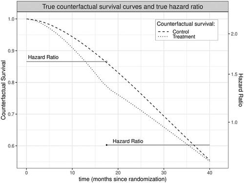
Because it compares event rates between study arms for participants who remain event-free at each moment, the hazard ratio can provide a misleading summary of the safety and efficacy of a treatment even in a perfectly executed trial of infinite sample size. To see why this is true, suppose a treatment increases the risk that a susceptible person will experience an event during early follow-up. Over time, the treatment arm will retain fewer and fewer high-risk individuals compared to the control arm; susceptibility to the outcome will thus no longer be balanced between arms by baseline randomization and the treatment arm will instead become increasingly advantaged. The hazard ratio, however, will continue to contrast these increasingly incomparable groups (Hernán 2010; Aalen, Cook, and Røysland 2015; Stensrud et al. 2019). Furthermore, the summary HR estimated by a Cox model is a weighted average of these potentially time-varying HRs (Moore and van der Laan 2009b). This means that when the hazard ratio varies across time, the true value of the Cox HR will depend on duration of follow-up, which easily differs among studies (Stensrud et al. 2017). In other words, with differing follow-up times the HR not only lacks a clear causal interpretation, how “noncausal” it is can vary between even perfectly executed trials enrolling identical populations. In the worst case, both the time-point specific HRs and their Cox-based summary may fail to capture the effect of treatment, for example leading to the conclusion that a treatment has a protective effect when it actually results in decreased survival probabilities throughout observed follow-up (Figure 1).

Figure 1: In this simulated dataset, treatment increases risk of an event early during follow up, depleting high risk persons in the treatment arm; as a result, the hazard among those still surviving at later time points is lower in the treatment versus control arm. Here, this scenario is exacerbated by informative drop-out. The summary hazard ratio from the Cox model implies a small protective effect of treatment (true Cox HR = 0.94, statistically significant at $\alpha =0.05$ in 61% of 1000 simulations using a sample size of 10,000), despite the fact that survival is actually lower in the treatment arm throughout follow up.

An immediate response to the scenario shown in Figure 1 might be that the Cox model would never be used when the proportional hazard assumption is so clearly violated. However, this only introduces another concern. With few exceptions, the primary statistical analysis of a RCT must be prespecified; post hoc specification of alternative approaches opens the door to spurious findings and is appropriately prohibited. Poorly understood informative drop out and violations of the proportional hazards assumption thus present challenges for prespecifying a Cox-based statistical analysis plan. Moreover, even if an analysis plan prespecifies tests for necessary assumptions and enumerates alternative models when the assumptions are clearly implausible, the limiting distributions of such composite estimators become nontrivial, thus, complicating reliable inference and communication of uncertainty. In the real-world, complexities such as competing risks (e.g., death from other causes), intercurrent events affected by post-randomization variables (e.g., treatment modification), and incomplete follow-up occur in even the best-conducted trials and these complexities can further undermine the plausibility that a Cox model adequately describes the data at hand.

Perhaps worse still, adherence to Cox coefficients as effect measures can have consequences even if the data is accurately described by a Cox model. Since Cox models assume censoring is independent of events given adjustment variables, researchers are rightly motivated to condition on covariates they know may predict informative dropout. However, the Cox model is non-collapsible and so adjusted Cox coefficients are not comparable to unadjusted Cox coefficients (Aalen, Cook, and Røysland 2015; Martinussen, Vansteelandt, and Andersen 2018; Daniel, Zhang, and Farewell 2021; Didelez and Stensrud 2022). This means that if researchers default to the Cox coefficient as their estimand, covariate adjustment choices not only impact bias and precision, but actually redefine the target estimand. In practice, well-meaning researchers interested in a marginal hazard ratio may thus feel forced into either using an unadjusted Cox model that is biased by informative censoring or an adjusted Cox model that does not estimate their parameter of interest. Additionally, attachment to the Cox coefficient as an estimand can discourage the inclusion of covariate-intervention interactions, even if doing so would be sensible given researchers’ knowledge of their data generating process. These complications and misunderstandings arise from the all-too-common practice of letting estimation choices dictate the estimand, but this need not, and ought not, be the case.

3 The Targeted Learning Roadmap

We suggest that the persistent, default use of Cox HR analyses stems from a common but risky approach: letting the data type dictate the statistical model, which in turn determines the estimand and the question being answered. Cox proportional hazard models provide a single measure of association and the ability to handle right censored time-to-event outcomes, so perhaps the implicit logic became: survival RCT data are straightforward to analyze with a Cox model and the output of a Cox model is a HR, therefore, the HR must be the quantity of interest. While concerns with this approach were later raised, they were often framed as statistical concerns with statistical remedies (such as weighted log-rank tests) (Lin et al. 2020). We suggest that rather than leaping from the motivating question—the safety and efficacy of new agents—immediately to the false comfort of a familiar statistical model, and by implication a statistical target quantity, we follow a roadmap to carefully guide a three-step process:

1. translation from a causal question about efficacy or safety to a formal target causal quantity defined in terms of an ideal hypothetical experiment;

2. translation from the target causal quantity to a target statistical quantity, while stating the necessary assumptions for doing so;

3. estimation of the target statistical quantity using a prespecified statistical approach that minimizes bias and maximizes precision while providing robust confidence intervals and reliable p-values.

Steps 1 and 2 are made possible by the formal causal frameworks (Cochran and Rubin 1973; Rubin 1974; Neyman, Dabrowska, and Speed 1990; Pearl 2000, 2009; Pearl, Glymour, and Jewell 2016) developed in past decades. The language of counterfactuals and of do-calculus are invaluable tools that can be applied to sharpen scientific questions (Step 1) and make transparent the assumptions necessary to answer these questions using observed data (Step 2). Explicitly stating these necessary assumptions facilitates discussions of their plausibility and opens a window for using sensitivity analysis to investigate the robustness of causal claims to their violations. This delineation of causal inference as a process separate from statistical estimation gives proper weight to the definition of interesting causal quantities and evaluation of necessary causal assumptions, and provides a structure for incorporating the limits of our knowledge into planning analyses and interpreting results.

For Step 3, we rely on the two-stage methodology of Targeted Maximum Likelihood Estimation (TMLE) (Moore and van der Laan 2009b; van der Laan and Rose 2011, 2018; Benkeser, Carone, and Gilbert 2018; Cai and van der Laan 2020). The first step of TMLE is to estimate necessary components of the data distribution, using machine learning to leverage baseline covariates in a flexible but prespecified way. Rarely, if ever, do we understand the world well enough to confidently prespecify a single regression model, deciding a priori which covariates to adjust for, in what way, and with which interactions. Machine learning provides a means to automate these decisions, responding to the actual data from the trial at hand in a fully prespecified way; rather than prespecifying the analysis decisions, we prespecify in software the decision process and thus remove any potential for bias caused by post hoc human intervention. While machine learning fits unknown functions in response to data and as a result produce less biased estimates as sample sizes increase, their precision also grows with sample size. Thus, as sample sizes increase, the shrinking bias can still result in misleading inferences, such as confidence intervals that exclude the truth. The second step of TMLE tackles this problem by updating the initial machine learning estimate to solve the estimand’s efficient influence function, thus, “targeting” the estimate for the statistical quantity of interest, restoring reliable statistical inference and optimizing precision and bias (Rubin 1974; Bickel et al. 1998; van der Laan and Robins 2003; van der Laan and Rose 2011, 2018). Further details regarding TMLE for survival probabilities are provided in Section 5.2.

In the following section we will demonstrate an application of the causal roadmap (Petersen and van der Laan 2014) to a hypothetical time-to-event RCT, modeled after the cardiovascular outcome trial LEADER. We begin, as always, by considering the causal question and defining a causal quantity of interest.

4 Data, Model, and Parameter of Interest

4.1 Causal Quantity

The first step of the causal roadmap (Petersen and van der Laan 2014) is to define the ideal hypothetical experiment that would allow the causal question of interest to be addressed. Here, we consider the following:

1. Assign all persons in the target population to the treatment and follow them without fail until either observing the event of interest or some maximum follow up time $t_{\max }$.

2. Assign all persons in the target population to the control and follow them without fail until either observing the event of interest or some maximum follow up time $t_{\max }$.

In the Neyman-Rubin causal model, (Cochran and Rubin 1973; Rubin 1974; Neyman, Dabrowska, and Speed 1990) these ideal, albeit impossible, conditions can be used to define a subject’s full data to include a collection of potential, or counterfactual, outcomes. Using this framework, we define the treatment-specific full data structure $X^a=(\mathbf{W},T^a)$, where $\mathbf{W}$ is a vector of baseline covariates, a is the hypothetical treatment, and $T^a$ is the counterfactual time to the failure event under treatment a. In the case of a typical RCT with one treatment arm and one control arm, the treatment variable is binary and thus the desired full data on a subject is defined as $X=(\mathbf{W},T^0,T^1)$. We should note that more complex ideal protocols can be defined for longitudinal RCTs, including hypothetical interventions to control regimen changes or drop-in treatments. If baseline covariates are sufficient to deconfound these treatment regimes from potential outcomes, then the following sections are still applicable with few modifications. However, time-varying treatments are usually subject to longitudinal confounding and though causal inference is still possible with those data structures, (Stitelman, De Gruttola, and van der Laan 2012; van der Laan and Rose 2018) this article will for brevity focus on data with a single treatment at baseline. Causal quantities of interest can then be defined as features of the distribution of this full data. For instance, the counterfactual probability of remaining event-free by time t under hypothetical intervention a is $$P(T^a>t)=\prod _{s=1}^t(1-{\lambda }^a(s)),$$where ${\lambda }^a(t)=P(T^a=t\mid T^a\ge t)$ is the counterfactual hazard and s takes whole number values from 1 through t. The corresponding counterfactual cumulative risk at t is $P(T^a\le t)=1-P(T^a>t)$. Typically though, causal quantities of interest compare the distributions of $T^1$ and $T^0$ in some way, such as the counterfactual difference in survival at time t, $P(T^1>t)-P(T^0>t)$; relative survival, $P(T^1>t) / P(T^0>t)$; or relative risk t, $P(T^1\le t) / P(T^0\le t)$. Each of these target quantities has merits: absolute survival and risk differences lend themselves to the clinically relevant Number Needed to Treat (NNT), while relative survivals and relative risks can highlight treatment effects on low incidence outcomes. In the absence of competing risks, whether to quantify survival or risk is a matter of clinical relevance, while in the presence of competing risks event-free survival should supplement rather than replace the outcome specific risk estimands. Since we will be re-analysing the LEADER trial which estimated a hazard ratio as its primary analysis, the following sections will focus on estimating the relative risk to allow a reasonable comparison to the hazard ratio. In a real trial analysis, the target quantity should be decided a priori on based on clinical relevance.

We might be only interested in these quantities at a single timepoint, for instance the last timepoint $t=t_{\max }$, but we might also be interested in these causal contrasts at any subset of times from time $t=1,\dots ,t_{\max }$, up to and including contrasts between the full survival curves. In such cases, we can define parameters that average the treatment effect over time, such as the time-averaged log hazard of survival proposed as a nonparametric extension of the Cox hazard ratio (Moore and van der Laan 2009b). (1) $$\Psi (P)=\frac{1}{t_{\max }}\sum _{t=1}^{t_{\max }}\hspace{0.17em}\log \hspace{0.17em}\left(\frac{\hspace{0.17em}\log \hspace{0.17em}\left(P(T^1>t)\right)}{\hspace{0.17em}\log \hspace{0.17em}\left(P(T^0>t)\right)}\right)$$(1)

However, time-averaged estimands obscure the dynamics of time-varying treatment effects, so instead we might estimate the causal target at multiple time points and then plot the parameter with simultaneous confidence bands over time. In a real trial, the choice of causal estimand should be driven by the clinical question, but in this article, to demonstrate the targeting of multiple time points using TMLE, we will define our target causal estimand as the relative risks of experiencing an event by the end of 12, 24, 36, and 48, months. $${\Psi }_t(P)=P(T^1\le t) / P(T^0\le t),t=12,24,36,48$$

As the analyses in this article were post hoc and meant solely for illustration, the targeted time points were chosen arbitrarily within reason; times were chosen to be late enough so that some events will have occurred and early enough so that some individuals are still at risk. The choice to target year-end risks was similarly arbitrary, compatible with the common preference for choosing “round” numbers and amenable to many time-coarsening options. For an actual analysis of trial data, target times should be pre-specified based on achievable follow up and clinical interest, not chosen ad hoc or post trial.

4.2 Observed Data

Let $T=T^A$ (the “consistency assumption” (Pearl 2010)) be a subject’s time to event and let C represent a subject’s time to censoring. We then denote an individual’s observed data by $O=(\mathbf{W},A,\tilde{T}=\min (C,T),\Delta =I(T\le C))$, where $\tilde{T}$ is the earlier of the subjects’ failure and censoring times, A is their randomly assigned treatment arm, and $\Delta$ is an indicator that the failure event was observed. This observed data structure is a function of the full data $(\mathbf{W},T^0,T^1)$ and “coarsening” variables $(A,C)$ and can also be represented in longitudinal form, $O=(\mathbf{W},A,N_c(t),N_1(t),t\le t_{\max })$ where $N_c(t)=I(\tilde{T}\le t,\Delta =0)$ and $N_1(t)=I(\tilde{T}\le t,\Delta =1)$. Here $N_1(t)$ is a counting process for the failure event, which jumps from 0 to 1 ($d{N}_1(t)=1$) at the time when a failure event is observed and $N_c(T)$ is an analogous counting process for censoring which jumps from 0 to 1 ($d{N}_c(t)=1$) at the onset of censoring. This longitudinal formulation for the observed data O then lends itself to the following factorization of the observed data likelihood for a single subject $O=o$: (2) $$\begin{array}{c}{P}_0(o)=P_W(w)\times P_A(a\mid w)\times \prod _{t=1}^{\tilde{t}}[P_{N_c(t)}\left(n_c(t)\mid w,a,\text{past}(t)\right)\\ \hspace{1em}\times P_{N_1(t)}\left(n_1(t)\mid w,a,n_c(t),\text{past}(t)\right)]\end{array}$$(2) where $\text{past}(t)=({\overline{n}}_c(t-1),{\overline{n}}_1(t-1))$, the histories of the censoring and failure counting processes up to but not including t, and t takes whole number values from 1 to the subject’s observed failure or censoring time $\tilde{t}$. Here $P_0$ is the distribution of observed data O, $P_W$ is the marginal distribution of covariates $\mathbf{W}$, $P_A$ is the conditional distribution of intervention A given $\mathbf{W}$; $P_{N_c(t)}$ is the conditional intensity of the censoring counting process $N_c(t)$ given $(\mathbf{W},A,\text{Past}(t))$; and $P_{N_1(t)}$ is the conditional intensity of the failure counting process $N_1(t)$ given $(\mathbf{W},A,N_c(t),\text{Past}(t))$. The likelihood of an observed data sample of n independent units $(o_1,\dots ,o_n)$ is then ${\prod }_{i=1}^{n}P(o_i)$, and the censoring and failure conditional hazards are, respectively (3) $$\begin{array}{cc}{\lambda }_c(t\mid \mathbf{W},A)\hfill & =P_{N_c(t)}(d{N}_c(t)=1\mid \tilde{T}\ge t,\mathbf{W},A)\hfill \end{array}$$(3) (4) $${\lambda }_1(t\mid \mathbf{W},A)=P_{N_1(t)}(d{N}_1(t)=1\mid \tilde{T}\ge t,\mathbf{W},A,N_c(t)).$$(4)

4.3 Identification

Translation of our target causal quantity, defined as a parameter of the distribution of counterfactual survival times (or hazards), into a parameter of this observed data distribution is possible under the following assumptions:

1. The randomization assumption (Robins 1986, 1999), that there is no unmeasured confounding of the effect of treatment on the counterfactual failure processes: $$A\perp \text{}\perp (T^0,T^1)\mid \mathbf{W}.$$

2. Coarsening at random on the conditional distribution of censoring given $(\mathbf{W},A,T)$ (Heitjan and Rubin 1991; Jacobsen and Keiding 1995; Gill, van der Laan, and Robins 1997), which can also be framed as a sequential randomization assumption: $$N_c(t)\perp \text{}\perp (T^0,T^1)\mid (\mathbf{W},A,{\overline{N}}_c(t),{\overline{N}}_1(t-1)),$$where again $\overline{X}(t)$ denotes the history of a variable X up to time t.

3. The “positivity assumption,” (Petersen et al. 2012) that adequate support for the target parameter exists in the underlying data distribution. For our relative risk estimand, $P(T^1\le t) / P(T^0\le t)$, we require that every subject has a nonzero probability of being assigned to both intervention and control irrespective of covariate values, and that every subject has a nonzero probability of remaining uncensored up until the latest target time point, irrespective of treatment and covariate values: $$P_A(a\mid \mathbf{W})>0,a\in \{0,1\}\text{-}\mathrm{a}.\mathrm{e}.;$$

and, $$1-{\lambda }_c(t\mid \mathbf{W},A)>0,t=0,\dots ,t_{\max }\text{-}\mathrm{a}.\mathrm{e}.$$

In a RCT, the randomization of treatment satisfies requirements 1 and 3 for positivity and unconfoundedness of treatment, while coarsening at random on censoring is satisfied if the conditional hazard of censoring at time t given $(\mathbf{W},A,T,C\ge t)$, depends only on the observed past at time t, $(\mathbf{W},A,{\overline{N}}_1(t),{\overline{N}}_c(t-1))$.

Under these assumptions on the treatment and censoring mechanisms, the post-intervention distribution of O under intervention $A=a$ in the world of no-censoring, that is, the distribution of $(\mathbf{W},T^a)$, can be represented by the G-computation formula (Robins 1986). Let us denote this post-intervention probability distribution with $P^a$ and the corresponding post-intervention random variable with $O^a$. The distribution of $O^a$ follows from replacing $P(A\mid \mathbf{W})$ by the intervention that sets A deterministically to a, and replacing the conditional probability of being censored at time t with an intervention that prevents censoring with probability 1. In notation, $P^1(O^1=o)$ is given by $$\begin{array}{cc}{P}^1(o)=P_W(w)\times I(a=1)\times \prod _{t=0}^{\tilde{t}}[I\left(n_c(t)=0\right)\hfill & \hfill \\ \hspace{1em}\times P_{N_1(t)}\left(n_1(t)\mid w,a,n_c(t),\text{past}(t)\right)].\hfill & \hfill \end{array}$$

Similarly, one can specify the post-intervention distribution $P^0$ under intervention $A=0$ in the world of no-censoring. Recalling the censoring (3) and conditional failure hazards (4) defined above in terms of the observed data and counting processes, given the above identifiability assumptions we have $$\begin{array}{cc}{\lambda }_c(t\mid \mathbf{W},A)=P_{N_c(t)}(d{N}_c(t)=1\mid C\ge t,\mathbf{W},A),\hfill & \hfill \\ {\lambda }_1(t\mid \mathbf{W},A)=P_{N_1(t)}(d{N}_1(t)=1\mid T\ge t,\mathbf{W},A),\hfill & \hfill \\ {\lambda }_1(t\mid \mathbf{W},A=a)=P(T^a=t\mid T^a\ge t,\mathbf{W}).\hfill & \hfill \end{array}$$

We note in particular, that the failure hazard is not conditional on censoring once the coarsening at random is assumed. We also note that $P_{N_1(t)}(n_1(t)\mid \tilde{T}\ge t,\mathbf{W},A)$ is equal to ${\lambda }_1(t\mid \mathbf{W},A)$ when $d{n}_1(t)=1$ and to $1-{\lambda }_1(t\mid \mathbf{W},A)$ when $d{n}_1(t)=0$, and analogously for $P_{N_c(t)}(n_c(t)\mid \tilde{T}\ge t,w,A)$. In other words, the observed data density $P(O=o)$ can be expressed in terms of the conditional failure and censoring hazards, and the post-intervention G-computation formula for $P(O^a=o)$ can be expressed in terms of the conditional failure hazard ${\lambda }_1(t\mid \mathbf{W},A)$. For example, the post-intervention density $P^1(O^1=o)$ can be equivalently written as $$\begin{array}{cc}{P}^1(o)=P_W(w)\times I(a=1)\times \prod _{t=0}^{\tilde{t}}[I\left(n_c(t)=0\right)\hfill & \hfill \\ \hspace{1em}\times {\lambda }_1{(t\mid w,a)}^{d{n}_1(t)}{(1-{\lambda }_1(t\mid w,a))}^{1-d{n}_1(t)}]\hfill & \hfill \end{array}$$and similarly for $P^0$. Since the density $P^a(O^a=o)$ implies any probability event about $O^a$, this G-computation formula for $P^a(O^a=o)$ also applies to causal quantities such as the survival probability under intervention $A=a$. Specifically, we can derive from the G-computation formula for $P^a(O^a=o)$ the following identification result for counterfactual survival at time t: (5) $$\begin{array}{c}P(T^a>t)=E_W\left[P(T>t\mid \mathbf{W},A=a)\right]\\ =E_W\left[\prod _{s=1}^t\left(1-{\lambda }_1(s\mid \mathbf{W},A=a)\right)\right]\mathrm{}.\end{array}$$(5)

The cumulative risk by time t is then simply given by $1-P(T^a>t)$.

4.4 Statistical Target Parameter

In Section 4.1 we considered potential causal target parameters: difference in survival probability $P(T^1>t) - P(T^0>t)$, relative survival $P(T^1>t) / P(T^0>t)$, and relative cumulative risk of failure $P(T^1\le t) / P(T^0\le t)$. These quantities all contrast timepoint-specific counterfactual survival probabilities under treatment versus control. With the above identification results for $P(T^a>t)$ and $P(T^a\le t)$, we can express these causal target quantities straightforwardly as parameters of the observed data distribution. Let ${\Psi }_t(P_0)$ denote the statistical target parameter defined based on such a contrast for a given time t. For our chosen target causal parameter of relative risk, $P(T^1\le t) / P(T^0\le t)$, we have the following identification result: (6) $$\begin{array}{cc}{\Psi }_t(P_0)=\left(1-E_W\left[\prod _{s=1}^t\left(1-{\lambda }_1(s\mid \mathbf{W},A=1)\right)\right]\right)\hfill & \hfill \\ \hspace{1em}/\left(1-E_W\left[\prod _{s=1}^t\left(1-{\lambda }_1(s\mid \mathbf{W},A=0)\right)\right]\right)\hfill & \hfill \end{array}$$(6) and more specifically, we are interested in this target parameter at the end of each of the first 4 years, $({\Psi }_t(P_0):t=12,24,36,48)$. We note that the target parameter ${\Psi }_t(P)$ is expressed only in terms of the conditional hazard ${\lambda }_1(t\mid \mathbf{W},A)$ and the marginal distribution of $\mathbf{W}$, so will use the alternative notation ${\Psi }_t(P_W,{\lambda }_1)$ to emphasize this point in later sections.

4.5 Statistical Model

At this stage along the causal roadmap, we have explicitly defined a causal parameter of interest and have stated the necessary assumptions for our causal parameter to be identified by the statistical target parameter ${\Psi }_t(P_0)={\Psi }_t(P_W,{\lambda }_1)$. It now remains to estimate this parameter by constructing estimators of the marginal distribution of $\mathbf{W}$, $P_W$, and of the conditional failure hazard ${\lambda }_1$. To do so, we must specify a statistical model $\mathcal{M}$ that reflects our knowledge about the different factors in the density factorization of $P_0(o)$ (2), and ensure that our estimators respect this knowledge as well as its limitations. For example, in a simple RCT setting we may know that treatment is completely randomized, such that the treatment mechanism is simply $P_A(A=1\mid \mathbf{W})=1/2$. Alternatively, we might know that a more complex randomization scheme such as stratified randomization was employed, which implies different model knowledge on the conditional distribution of treatment assignment. In some cases we might also have knowledge on the conditional hazard of censoring, for instance that we can safely assume censoring at time t is unaffected by treatment and covariates, in which case ${\lambda }_c(t\mid A,\mathbf{W})={\lambda }_c(t)$. Regarding the conditional failure hazard there is generally no reliable knowledge, but should we have relevant domain knowledge (e.g., upper bounds on failure incidence), it would be incorporated in the statistical model at this stage and thereby into the subsequent estimation process.

4.6 Statistical Estimation Problem

The statistical estimation problem is now defined as follows: (a) we observed n iid observations $O_1,\dots ,O_n$ from probability distribution $P_0$; 2) we specified our target estimand ${\Psi }_t(P_0)$; and 3) we specified our knowledge about the distribution $P_0$ by setting down a statistical model $\mathcal{M}$, defined as the set of possible probability distributions $P_0(O)$. What remains is to estimate ${\Psi }_t(P_0)$ and to provide statistical inference in terms of confidence intervals with nominal coverage and formal testing of null-hypotheses with Type 1 error control.

5 Estimation

As we can see in (4.4), the target parameter ${\Psi }_t(P_W,{\lambda }_1)$ only depends on the marginal distribution of $\mathbf{W}$ through an expectation of a function of $\mathbf{W}$. Therefore, in defining an estimator of our target statistical parameter, we can simply estimate this expectation $E_W$ with the empirical mean. To finish defining a plug-in estimator based on (4.4), all that remains is to construct an estimator of the failure conditional hazard, ${\lambda }_1$. Below we describe two plug-in estimators, G-computation (Robins 1986) and Targeted Maximum Likelihood Estimation (TMLE) (van der Laan and Rubin 2006; van der Laan and Rose 2011, 2018; Benkeser, Carone, and Gilbert 2018; Cai and van der Laan 2020). Benkeser et al. (2020) provide a recent review of the literature on this and other covariate adjustment methods (including robust and efficient methods for RCTs with time-to-event outcomes) and evaluate their application in the context of COVID-19 trials.

5.1 G-Computation

If we understood the failure event’s conditional hazard function sufficiently to safely assume that it followed, for instance, a Cox proportional hazards model, we could fit the appropriate model and rely on maximum likelihood estimation theory for inference. Analogously in our discrete time formulation, if we were able to commit to a logistic model of the discrete hazard, then we could take a pooled repeated observations approach (what Efron (1988) describes as partial logistic regression). For instance we might believe that the true model has the following simple structure, (7) $$\hspace{0.17em}\log \hspace{0.17em}\left(\frac{{\lambda }_1(t\mid \mathbf{W},A)}{1-{\lambda }_1(t\mid \mathbf{W},A)}\right)={\alpha }_0+{\theta }_t+\mathbf{W}\beta +A\gamma$$(7) where ${\alpha }_0$ is the intercept, ${\theta }_t$ is the effect of time t, $\beta$ is the effect of covariates, and $\gamma$ is the effect of treatment. We note that since our estimand is not defined as a model coefficient, we could easily extend the model to include treatment interactions without introducing complications with effect interpretation. Estimates of treated or control survival are calculated by replacing ${\lambda }_1$ in (5) with an estimate, ${\widehat{\lambda }}_1$, and taking an empirical mean over observed w in place of the expectation $E_W$. Estimating ${\Psi }_t(P_0)$ given the treated and control survival probabilities is then a straightforward application of the delta method.

Often, however, there is no compelling reason to suppose that the conditional hazard of failure lies in any particular parametric model (a fact that would be made explicit during the process of specifying a statistical model on the roadmap). As a consequence, while we might choose to estimate the parameters of a parametric or semiparametric hazard model, such as those described above, with maximum likelihood, we cannot rely on the theory of maximum likelihood estimation for parametric models as our basis for inference. In practice, the variance of such G-computation estimators is often estimated using a nonparametric bootstrap, but model misspecification will lead to a bias that does not disappear with increasing sample size.

5.2 TMLE

When working in large statistical models that potentially make assumptions only on the conditional distribution of treatment or conditional hazard of censoring, we rely on semi-parametric efficiency theory developed for these larger statistical models (Bickel et al. 1998). From this theory we learn that a regular estimator for a statistical target parameter in a semiparametric model is asymptotically efficient (i.e., with minimal asymptotic variance) if it is asymptotically linear with influence function equal to the Efficient Influence Curve (EIC), where the asymptotic linearity condition requires that the estimator minus target parameter can be expressed as the sample mean of a random variable over the n observations $(O_1,\dots ,O_n)$, up to an asymptotically vanishing second order remainder. This EIC is defined as the canonical gradient of the pathwise derivative of ${\Psi }_t(P_0)$. Importantly, the canonical gradient represents the score at $ϵ=0$ of a one-dimensional path through $P_0$, $(P_{ϵ}:ϵ)$, along which the normalized derivative $d/dt{\Psi }_t(P_{ϵ})$ at $ϵ=0$ is maximal. Such a path is called a least favorable parametric submodel since it represents a parametric model under which the maximum likelihood estimator of ${\Psi }_t(P_{ϵ})$ has the largest asymptotic variance. This least favorable parametric submodel is used by TMLE to construct an efficient estimator of the target parameter.

A prerequisite for implementing any TMLE is therefore to first obtain the relevant canonical gradient, as it provides a key ingredient for the construction of an efficient estimator. Calculating this canonical gradient requires functional Hilbert space calculations, but for many problems (as in the case for survival and cumulative risk target parameters) this work has already been done (Robins and Rotnitzky 1992; van der Laan and Robins 2003; Moore and van der Laan 2009b). The two-stage TMLE process then proceeds in this general form: first construct an initial estimator $\widehat{P}$ of the observed data density $P_0$, and then use a maximum likelihood estimator for the least favorable path through this initial estimator ($\{{\widehat{P}}_{ϵ}:ϵ\}$) to update the initial estimate of the density. The updated density estimate is then simply plugged in to produce ${\Psi }_t({\widehat{P}}_{{ϵ}_n})$, the estimator of the target parameter ${\Psi }_t(P_0)$ where ${ϵ}_n$ is the MLE of $ϵ$.

For the initial TMLE step, the stacked ensemble machine-learning method of Super Learner, has in particular been successfully employed (van der Laan and Rose 2011, 2018). As it is impossible to know a priori which type of algorithm is best suited for fitting as yet unseen data, Super Learner instead evaluates a range of algorithms by using internal sample splitting (typically 10-fold cross-validation) performance to choose the combination of algorithms that performs best with the data at hand (van der Laan and Rose 2011, 2018). The importance of specifying a suitable Super Learner library should not be understated, as TMLE will not retain its desirable properties if all candidate models badly underfit or overfit the data. Though thoughtful candidate library construction can mitigate the risk of global underfitting and the cross-validated discrete Super Learner selector can mitigate the risk of overfitting, we advise evaluating any proposed settings on simulations that emulate the size and summary characteristics of the actual data. For instance, the typical 10-fold cross-validation structure has seen to perform well generally, but with smaller samples sizes, for example, $N\le 100$, increasing the number of folds may improve performance. Super Learner loss functions should be bounded and minimized at the target truth, and candidate libraries should contain models that range in flexibility. For estimating conditional hazards, a good library might range from small parametric models such as an unadjusted Cox to more flexible machine learning algorithms such as Cox glmnet (Simon et al. 2011). Alternatively, one might construct a library of increasingly flexible highly adaptive LASSO (HAL) models, thus, not only producing a library with models of varied flexibility but also solving many score equations with a fast convergence rate (Benkeser and van der Laan 2016). Ultimately, well specified Super Learners allow for flexible and prespecified estimation, but when used alone do not typically achieve the balance between bias and variance needed for reliable inference, thus, necessitating the following targeting step (van der Laan and Rubin 2006).

In the second step, the initial machine learning estimate is updated in a process that sometimes relies on estimates of so-called nuisance parameters. In the example of estimating relative cumulative risk, the initial conditional hazard fit is updated using estimates of two additional quantities: the randomization probability given covariates (a known function in a RCT) and the probability of right-censoring given covariates and trial arm. In common with other semiparametric efficient estimators (Benkeser et al. 2020), TMLE is double robust in consistency if either (a) the treatment mechanism and censoring mechanism are consistently estimated or (b) the failure time hazard is consistently estimated. In RCTs, the conditions for (a) can often be reasonably established without reliance on machine learning, at least with respect to the treatment mechanism, while condition (b) will generally require data-adaptive estimation using machine learning. A full discussion of assumptions required for asymptotic linearity are provided elsewhere (Bickel et al. 1998; van der Laan and Robins 2003; van der Laan and Rubin 2006; van der Laan 2017; van der Laan and Rose 2018) but in short, asymptotic inference for TMLE is based on solving EICs and relies on initial estimators that (i) do not badly overfit and (ii) converge adequately quickly. More specifically, the first requirement is that the initial estimators fall in a Donsker class, though this requirement can be circumvented by cross-validated TMLE (van der Laan 2017; van der Laan and Rose 2018). The second requirement is that for TMLE to be efficient, the product of the convergence rates of the intervention-related estimators and the outcome-related estimators must be at least $n^{-1/2}$. This is the motivation for estimating nuisance parameters using Super Learner; its oracle convergence property works with well-specified candidate libraries to give the best chance at attaining the necessary rate. In particular, a TMLE using Super Learners that include HAL, which attains a convergence rate of $n^{-1/3}$ up til $\log (n)$ factors, Bibaut and van der Laan (2019) is asymptotically efficient assuming only strong positivity (van der Laan 2017; van der Laan and Rose 2018). Otherwise, in RCTs if only one of either the censoring or the outcome processes is consistently estimated, TMLE will still be consistent with conservative IC-based inference as can be seen by the conservative coverage of the TMLEs with misspecified hazard models in our simulations (Tables 2 and 4). Importantly, this means that asymptotic inference and type-1 error control of TMLE is not directly dependent on uncertainty in nuisance parameter estimation; this is a crucial benefit of TMLE’s targeting step.

Table 2: Estimator performance under non-informative censoring, with sample size n = 1000 over 1000 iterations: 95% coverage is calculated using the estimators’ estimated standard error, which is not directly available for these G-computation estimators.

Estimand	Estimator	Hazard	Bias	95% Cov. (Sim)	Rel. Efficiency	Rel. MSE
Control Surv.	KM	NA	0.00	0.95 (0.95)	1.00	1.00
	G-Comp	Misspecified	0.03	NA (0.62)	1.09	0.28
		SuperLearner	0.00	NA (0.94)	1.59	1.56
	TMLE	Misspecified	0.00	0.97 (0.96)	1.17	1.17
		SuperLearner	0.00	0.96 (0.96)	1.17	1.17
Treated Surv.	KM	NA	0.00	0.94 (0.94)	1.00	1.00
	G-Comp	Misspecified	0.04	NA (0.35)	1.37	0.21
		SuperLearner	−0.01	NA (0.89)	1.46	0.96
	TMLE	Misspecified	0.00	0.97 (0.95)	1.20	1.20
		SuperLearner	0.00	0.95 (0.95)	1.21	1.21
Risk Diff.	KM	NA	0.00	0.95 (0.95)	1.00	1.00
	G-Comp	Misspecified	–0.01	NA (0.94)	1.24	1.13
		SuperLearner	0.01	NA (0.92)	2.12	1.67
	TMLE	Misspecified	0.00	0.98 (0.95)	1.41	1.41
		SuperLearner	0.00	0.95 (0.95)	1.40	1.40
Rel. Risk	KM	NA	0.00	0.94 (0.94)	1.00	1.00
	G-Comp	Misspecified	–0.04	NA (0.88)	1.18	0.72
		SuperLearner	0.02	NA (0.91)	2.03	1.46
	TMLE	Misspecified	0.00	0.98 (0.95)	1.40	1.40
		SuperLearner	0.00	0.94 (0.95)	1.40	1.40
Rel. Surv.	KM	NA	0.01	0.96 (0.95)	1.00	1.00
	G-Comp	Misspecified	–0.01	NA (0.95)	1.41	1.41
		SuperLearner	–0.02	NA (0.94)	2.15	1.90
	TMLE	Misspecified	0.00	0.98 (0.96)	1.39	1.39
		SuperLearner	0.01	0.96 (0.95)	1.38	1.38

NOTE: In parentheses is the coverage based on the estimators’ standard errors in this simulation. Relative efficiency (higher is better) is calculated as var(KM)/var(Est) and relative MSE (higher is better) is calculated as MSE(KM)/MSE(Est), respectively. True estimands: S₀ = 0.43, S₁ = 0.60, RD = $-$0.17, RR = 0.70, RS: 1.40

Table 4: Estimator performance under informative censoring, with sample size $n=1000$ over 1000 iterations: 95% coverage is calculated using the estimators’ estimated standard error, which is not directly available for these G-computation estimators.

Estimand	Estimator	Hazard	Bias	95% Cov. (Sim)	Rel. efficiency	Rel. MSE
Control Surv.	KM	NA	0.01	0.94 (0.94)	1.00	1.00
	G-Comp	Misspecified	0.05	NA (0.33)	1.32	0.21
		SuperLearner	0.00	NA (0.96)	1.57	1.75
	TMLE	Misspecified	0.00	0.98 (0.95)	1.12	1.25
		SuperLearner	0.00	0.96 (0.96)	1.14	1.27
Treated Surv.	KM	NA	0.04	0.62 (0.60)	1.00	1.00
	G-Comp	Misspecified	0.08	NA (0.04)	1.24	0.35
		SuperLearner	0.00	NA (0.95)	1.69	6.39
	TMLE	Misspecified	0.01	0.96 (0.94)	1.14	3.92
		SuperLearner	0.00	0.96 (0.96)	1.20	4.64
Risk Diff.	KM	NA	–0.03	0.86 (0.83)	1.00	1.00
	G-Comp	Misspecified	–0.03	NA (0.82)	1.23	1.26
		SuperLearner	0.00	NA (0.93)	2.38	4.80
	TMLE	Misspecified	–0.01	0.98 (0.94)	1.36	2.62
		SuperLearner	0.00	0.95 (0.95)	1.41	2.89
Rel. Risk	KM	NA	–0.07	0.84 (0.85)	1.00	1.00
	G-Comp	Misspecified	–0.06	NA (0.87)	1.02	1.18
		SuperLearner	0.01	NA (0.96)	2.32	4.31
	TMLE	Misspecified	–0.01	0.98 (0.94)	1.32	2.42
		SuperLearner	0.00	0.94 (0.95)	1.35	2.58
Rel. Surv.	KM	NA	0.06	0.87 (0.82)	1.00	1.00
	G-Comp	Misspecified	0.05	NA (0.78)	1.41	1.30
		SuperLearner	–0.01	NA (0.93)	2.43	5.18
	TMLE	Misspecified	0.01	0.98 (0.94)	1.39	2.77
		SuperLearner	0.00	0.95 (0.95)	1.45	3.14

NOTE: In parentheses is the coverage based on the estimators’ standard errors in this simulation. Relative Efficiency (higher is better) and Relative MSE (higher is better) of estimators is with respect to Kaplan-Meier, var(KM)/var(Est) and MSE(KM)/MSE(Est), respectively. True Estimands: S₀ = 0.56, S₁ = 0.52, RD = 0.04, RR = 1.09, RS = 0.93.

5.2.1 TMLE for Right-Censored Survival

When considering the relevant canonical gradient for our relative risk target estimand (4.4), we can simplify by targeting the treatment-specific survival curves instead. Inference for these treatment-specific survival estimates can then be easily transformed using the delta method into inference on relative risks or other survival curve-derived estimands. Thus, we begin here with the canonical gradient for the treatment-specific survivals at a target time $\tau$, ${\tilde{\Psi }}_{\tau }^a(P_0)=E_W\left[{\prod }_{t=1}^{\tau }(1-{\lambda }_1(t\mid \mathbf{W},A=a))\right]$ for $a=0,1$: (8) $$\begin{array}{cc}{D}_a^{*}(P_0)(O)=\sum _{t=1}^{\tau }I(t\le \tilde{T}) H_{a,\tau }^{*}(t,A,\mathbf{W})\left(d{N}_1(t)-{\lambda }_1(t\mid A,\mathbf{W})\right)\hfill & \hfill \\ \hspace{1em}+S(\tau \mid A=a,\mathbf{W})-{\tilde{\Psi }}_{\tau }^a(P_0)\hfill & \hfill \end{array}$$(8) where (9) $$\begin{array}{c}\begin{array}{cc}{H}_{a,\tau }^{*}(t,A,\mathbf{W})\hfill & =0\left(\frac{I(A=a)I(t\le \tau )}{P_A(a\mid \mathbf{W})S_c(t^{\mathrm{ }\_}\mid a,\mathbf{W})}\right)\left(\frac{S(\tau \mid a,\mathbf{W})}{S(t\mid a,\mathbf{W})}\right),\hfill \end{array}\\ S(t\mid a,\mathbf{W})=\prod _{v=1}^t(1-{\lambda }_1\left(v\mid a,\mathbf{W}\right))\hspace{1em}\mathrm{ }\text{and}\mathrm{ }\\ S_c(t\mid a,\mathbf{W})=\prod _{v=1}^t(1-{\lambda }_c\left(v\mid a,\mathbf{W}\right))\end{array}$$(9)

TMLE for our target parameter ${\tilde{\Psi }}_{\tau }^a(P_W,{\lambda }_1)$ then proceeds by generating initial estimates for $P_W$ and ${\lambda }_1$. Next this initial estimate, $\widehat{P}=({\widehat{P}}_W,{\widehat{\lambda }}_1)$, is updated by MLE along the least favorable parametric submodel through $\widehat{P}$ to produce the updated estimate ${\widehat{P}}_{{ϵ}_n}=({\widehat{P}}_W,{\widehat{\lambda }}_{1,{ϵ}_n}$). We note that ${\widehat{P}}_W$ is the empirical distribution, so as a nonparametric MLE is not changed in the update process. The updated hazard estimate takes the form $$\text{logit}{\widehat{\lambda }}_{1,{ϵ}_n}(t\mid A,\mathbf{W})=\text{logit}{\widehat{\lambda }}_1(t\mid A,\mathbf{W})+ϵ h_{a,\tau ,n}^{*}(t,A,\mathbf{W})$$where $h_{a,\tau ,n}^{*}(t,A,\mathbf{W})$ is the estimate of $H_{a,\tau }^{*}(t,A,\mathbf{W})$ (9). In iterated TMLE, the updated hazard ${\widehat{\lambda }}_{1,{ϵ}_n}$ would then be used as the “initial” offset for the next update step, until the mean of the empirical EIC is less than or equal to the standard error of the EIC divided by $\log (n) \sqrt{n}$, where n is the number of observations. The final updated hazard estimate we denote as ${\widehat{\lambda }}_{1,{ϵ}_n}^{*}$. The updated estimates ${\widehat{P}}_{{ϵ}_n}=({\widehat{P}}_W,{\widehat{\lambda }}_{1,{ϵ}_n}^{*}$) are then used in a plug-in estimator: (10) $${\tilde{\Psi }}_{\tau }^a({\widehat{P}}_{{ϵ}_n})=\frac{1}{n}\sum _i\left[\prod _{t\mathrm{ }\le \tau }\left(1-{\widehat{\lambda }}_{1,{ϵ}_n}^{*}(t\mid \mathbf{W},A=a)\right)\right]\mathrm{}.$$(10)

As a plug-in estimator, ${\tilde{\Psi }}_{\tau }^a({\widehat{P}}_{{ϵ}_n})$ respects global constraints and by fluctuating with respect to a vector of time-dependent clever covariates corresponding with many time points, a one-step TMLE targeting the survival curve at multiple time points further ensures that the created curve remains bounded in [0, 1] and is monotone decreasing, while still being asymptotically efficient given regularity conditions on the initial estimators (van der Laan and Rose 2018; Cai and van der Laan 2020). Under these conditions the TMLE is regular and asymptotically linear with influence curve equal to the efficient influence curve (van der Laan and Rose 2011, 2018), which implies by the CLT implies that the TMLE converges to a Gaussian distribution. As with other semi-parametric efficient estimators, (Robins and Rotnitzky 1992; Bickel et al. 1998; van der Laan and Robins 2003) when the initial estimators of the failure hazard, the treatment mechanism, and the censoring mechanism are consistent with respect to their true counterparts, the variance of the normal limiting distribution is the variance of the EIC and can be naturally estimated by the sample variance of the EIC. This leads familiarly both to Wald-type testing and the construction of confidence intervals, and indeed simultaneous confidence intervals if one is so interested.

6 Implementation

6.1 Software

Analyses in this article were performed using the survtmle R package (Benkeser, Carone, and Gilbert 2018) which enables estimation of survival probabilities at single time points via G-computation and TMLE. Modifications were made to survtmle’s native functions, the most significant of which was to allow the TMLE to simultaneously target multiple time-points (Moore and van der Laan 2009b; van der Laan and Rose 2011; Cai and van der Laan 2020). The modified code and all necessary code for producing the following simulation results are available on Github (https://github.com/imbroglio-dc/Roadmap_CVOT). Code for the primary and subgroup LEADER trial analysis is also available, though the LEADER dataset is not included.

7 Simulation Studies

To demonstrate the finite sample performance of the G-computation and TMLE estimators described in Sections 5, together with a standard Kaplan-Meier estimator, we performed a pair of simulations. In the first simulation we examined a hypothetical trial with independent right censoring while in the second we considered one in which censoring differed systematically between trial arms. In order to present a realistic picture of the performance of the G-computation and TMLE estimators, we estimated the conditional hazard of failure with three “strategies”: a) an “optimistic” correctly specified pooled logistic regression, (b) a “low effort” misspecified, main-terms pooled logistic regression, and (c) a “realistic” Super Learner using a modest library of well-known algorithms: logistic regression (stats::glm), penalized logistic regression (glmnet), Bayesian logistic regression (arms::bayesglm), gradient boosting (xgboost), and random forest (ranger). These candidate models were used with their respective package defaults and in the interest of brevity we will not exhaustively detail those settings here; for further detail, the code for all analyses are available in the accompanying github repository and further explanations of model settings are best explained in their respective package documentations. In both simulations the conditional hazard of censoring was estimated with Super Learner using a library similar to that specified above, and propensity score was estimated using a simple main terms logistic regression. All Super Learners used simple 10-fold cross-validation with negative log-likelihood loss and a convex combination meta-learner as the Super Learner selector.

One cautionary note we make is that when events are rare, which can be exacerbated by finely discretized time scales, the repeated measures pooled logistic regression approach can be unstable. One common method to address this limitation is to coarsen the time scale, which we employ here by binning the data into four month intervals. This approach also has the added benefit of reducing needed computation time and resources, but provides lower temporal resolution and can introduce bias if the desired analysis incorporates adjusting for time-varying covariates or treatment. Excessive time coarsening can also cause complications since later censoring events within a coarsened interval will be treated as occurring at the start of the interval. A continuous time TMLE, for instance utilizing Cox regressions to estimate conditional hazards, would avoid these issues while simultaneously reducing computational cost (Rytgaard, Eriksson, and van der Laan 2021).

Each simulation consisted of 1000 samples of size $n=1000$. 11 Baseline covariates were pulled from the LEADER trial (Marso et al. 2016) (Table 1) and treatment assignments were generated from a Bernoulli distribution with $p=0.5$. Failure and censoring events in the two simulations were generated in discrete time with hazard functions which will be detailed in subsequent sections. These hazard functions were chosen for simplicity, to produce a reasonable number of events by the target time with moderately predictive covariates and a treatment interaction. Many alternative and potentially more complicated data-generating processes are also possible, but these simple simulations are sufficient to display the estimators’ general properties. The target parameters in both simulations were the treated and control survivals at an arbitrarily chosen $t=104$ (year 2 on a weekly scale) from which we then compute difference in survival, relative survival, and relative risk. Kaplan-Meier, G-computation, and TMLE estimators are compared across these target estimands and, for G-computation and TMLE, across the three conditional hazard estimation specifications. Rather than targeting multiple time points, a single time point was targeted in these simulations to reduce computational cost. Variance estimation for the Kaplan Meier estimator variance estimation was based on Greenwood’s formula, (Greenwood 1926) while inference for TMLE was computed from the variance of the influence curve. Coverage for the G-computation estimator was not calculated since the typical bootstrap method for calculating its variance would be computationally costly in iterated simulations. So-called “oracle coverage” was also calculated for each estimator based on their respective standard errors in each simulation.

Table 1: LEADER Baseline Covariates used for simulations.

Variable	Description
Region	Categorical: Asia, E. Europe, W. Europe, N. America, Other
Age	Numerical: years
Sex	Logical: 1 - Male, 0 - Female
Ethnicity	Logical: 1 - White, 0 - Other
MI	Logical: Myocardial Infarction Flag at Baseline
Smoker	Logical: Smoker Status at Baseline
Stroke	Logical: Stroke Flag at Baseline
eGFR	Numerical: eGFR at Baseline using the CKD-EPI formula
Creatinine	Numerical: serum creatinine at Baseline
BMI	Numerical: Body Mass Index at Baseline
HbA1c	Numerical: HbA1c at Baseline (SI)

NOTE: NOTE: Correlation between eGFR and creatinine is not a concern as the Super Learner algorithm operates only with the candidate model predictions.

7.1 Noninformative Censoring

Failure events for the noninformative censoring simulation were generated with the hazard function $$\begin{array}{cc}\lambda (t)=0.002\hspace{0.17em}\exp \hspace{0.17em}( 2.2\times W_{\text{Smoker}}+0.4\times A\times W_{\text{Smoker}}\hfill & \hfill \\ \hspace{1em}+.7\times {(-1)}^A\times W_{\text{Obese}}).\hfill & \hfill \end{array}$$

Censoring events for both treatment and control arms were generated from a Kaplan-Meier fit of the observed censoring events in the LEADER trial.

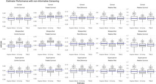
Figure 2 and Table 2 show the simulation results for the Kaplan-Meier, G-computation, and TMLE estimators in a simulation with noninformative right censoring. With independent censoring and predictive covariates, we expect the Kaplan-Meier and TMLE estimators to be unbiased, and for TMLE to show improved efficiency relative to Kaplan-Meier. Indeed we see this pattern throughout Figure 2 and Table 2. The relative efficiency of TMLE with initial estimation using Super Learner (TMLE + SL) compared to Kaplan-Meier ranged from a minimum of 1.14 for control survival to 1.32 for relative risk. Since both Kaplan-Meier and TMLE exhibit negligible bias, as is expected given the non-informative censoring, the mean squared errors of the TMLEs were also lower across the five target parameters (control survival, treated survival, risk difference, relative risk, relative survival) with magnitudes mirroring TMLE’s precision improvement over Kaplan-Meier. Table 2 and Figure 2 also illustrate how the G-computation estimator relies on correct model specification for good performance. Although the G-computation estimator using a correctly specified parametric model (top row of Figure 2) outperforms both Kaplan-Meier and TMLE, when the data generating process lies outside of the specified model (Table 2 and the middle and bottom rows of Figure 2) the G-computation estimator is subject to non-negligible bias and misleading inference. We can further see in Table 2 and Figure 2 that the degree of model misspecification determines the severity of the G-computation estimator’s bias: the G-computation estimator using a badly misspecified model (model adjusting for treatment only) is more severely biased than the G-computation estimator using a Super Learner of moderately misspecified models (models missing treatment interactions). Though G-computation estimators can at best outperform other estimators, their reliance on correct model specification makes them poorly suited for real world applications where the true data-generating mechanism is unknown and reliable inference is desired. In fact, the G-computation estimator’s precision makes false positives more likely when the estimator is biased, as seen in Table 2 where the 95% oracle coverage (coverage calculated using the estimators’ simulation variance) for the Super Learner G-computation estimator falls between 0.89 and 0.94 while the coverage of the misspecified G-computation estimator drops as low as 0.35. In contrast TMLE displayed its “double robustness” property, remaining unbiased and retaining nominal confidence interval coverage despite using the same badly misspecified hazard model to initially fit the conditional hazard of failure.

Figure 2: Estimator performance under non-informative censoring. Box-plots show estimators’ mean and 25–75% quantiles. Text boxes show coverage of 95% confidence intervals. Columns (left to right): Control Survival, Treated Survival, Risk Difference, Relative Risk, and Relative Survival Rows: Top—correct hazard model, Middle—misspecified hazard model, Bottom—SuperLearner ensemble The effect of model misspecification on G-computation estimators can be seen in the misspecified hazard (middle) and SuperLearner (bottom) rows, while in the same rows we see that TMLE is able to compensate for model misspecification. Kaplan-Meier is expected to be consistent in this independent censoring scenario, but TMLE can be seen throughout to provide mild efficiency gains.

Here we also note that the degree to which a well-specified TMLE will outperform Kaplan-Meier in the absence of informative censoring is related to the ability of the covariates in predicting outcomes. For example, when we multiply the covariate coefficients in this noninformative censoring simulation by approximately a factor of 3, relative efficiency gain of TMLE + SL over Kaplan-Meier increases to 1.24 for control survival and 1.51 for relative risk. On the other hand if we decrease the predictive power of the covariates by approximately a factor of 3, the relative efficiency gain of TMLE with Super Learner over Kaplan-Meier shrinks to 1.03 for control survival and 1.09 for relative risk. These results are summarized in Table 3, which shows that across all estimands and covariate predictiveness conditions, TMLE remains practically unbiased with reliable 95% confidence interval coverage. Across all estimands, the relative efficiency of TMLE compared to Kaplan-Meier grows with increasing covariate predictiveness while the relative MSE of Kaplan-Meier is greater than TMLE by almost exactly the same ratio. This is again expected, as both estimators are unbiased and thus the increased relative MSE of Kaplan-Meier over TMLE is driven by the higher variance of the Kaplan-Meier estimator.

Table 3: The performance of TMLE using Superlearner versus Kaplan-Meier with non-informative censoring under different covariate predictiveness conditions: Medium is the hazard function as shown in Section 7.1, Low divides those covariate coefficients by $\sim$3 while High multiplies the covariate coefficients by $\sim$3.

Estimand	Predictiveness	Truth	TMLE Bias	Rel. Eff	Rel. MSE	TMLE 95% cov
Control survival	Low	0.756	0.001	1.03	1.03	0.95
	Medium	0.430	0.000	1.13	1.13	0.95
	High	0.291	–0.001	1.24	1.24	0.95
Treated survival	Low	0.821	–0.001	1.06	1.06	0.94
	Medium	0.601	–0.001	1.18	1.17	0.94
	High	0.493	–0.001	1.24	1.24	0.95
Risk difference	Low	−0.065	0.002	1.09	1.09	0.95
	Medium	−0.172	0.001	1.31	1.31	0.95
	High	−0.202	–0.001	1.52	1.52	0.94
Relative risk	Low	0.734	0.010	1.10	1.10	0.95
	Medium	0.699	0.002	1.31	1.31	0.94
	High	0.715	0.000	1.48	1.48	0.94
Relative survival	Low	1.090	–0.002	1.09	1.09	0.95
	Medium	1.400	0.001	1.28	1.28	0.94
	High	1.690	0.011	1.51	1.51	0.95

NOTE: Relative Efficiency is calculated by dividing the Kaplan-Meier variance by the TMLE variance and relative MSE is calculated by dividing the MSE of Kaplan-Meier over TMLE.

7.2 Informative Censoring

Failure events for the informative censoring simulation were generated with the hazard function $${\lambda }_1(t)=0.0015\hspace{0.17em}\exp \hspace{0.17em}(2.8\times W_{\text{Smoker}}+0.4\times A\times W_{\text{Smoker}})$$

Censoring events in this simulation were generated from the following: $$\begin{array}{cc}{\lambda }_c(t)=\text{KM}(t)\times \hspace{0.17em}\exp \hspace{0.17em}(1.1\times I(A=0)\times W_{\text{Smoker}}+2.8\hfill & \hfill \\ \hspace{1em}\times I(A=1)\times W_{\text{Smoker}})\hfill & \hfill \end{array}$$where KM is the same Kaplan-Meier fit of observed censoring events in the LEADER trial that was used in the non-informative censoring simulation.

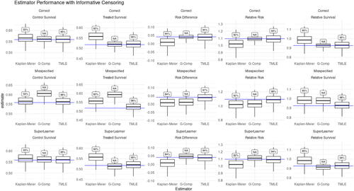
Figure 3 and Table 4 show the simulation results for the Kaplan-Meier, G-computation, and TMLE estimators in the presence of informative censoring. Since censoring is now informative, we no longer expect the Kaplan-Meier estimator to be unbiased, and indeed this is reflected throughout Figure 3 as well as in the bias and drop in 95% confidence interval coverage reported in Table 4. Comparing the performance of the G-computation estimator in Table 4 and across the rows of Figure 3 continues to illustrate the sensitivity of the G-computation estimator to model misspecification. TMLE in contrast continues to correct for the bias introduced by using misspecified parametric models to estimate the conditional hazard of failure. One might also notice that compared to its performance in the prior non-informative censoring simulation, the Super Learner based G-computation estimator seems to perform better in the presence of informative censoring. This is coincidental to our simulations and reflects the fact that by chance our Super Learner fit the informative censoring data better than it did the non-informative censoring data. To illustrate that this is not a reliable property of the G-computation estimator, the G-computation estimator based on a simple misspecified hazard had much poorer oracle coverage in the informative censoring simulation (0.04 and 0.87) than it did in the non-informative censoring simulation (0.35 and 0.95).

Figure 3: Estimator performance under Informative Censoring. Box-plots show estimators’ mean and 25–75% quantiles. Text boxes show coverage of 95% confidence intervals. Columns (left to right): Control Survival, Treated Survival, Risk Difference, Relative Risk, and Relative Survival Rows: Top—correct hazard model, Middle—misspecified hazard model, Bottom—SuperLearner The effect of model misspecification on G-computation estimators can be seen in the misspecified hazard (middle) and SuperLearner (bottom) rows, while in the same rows we can see TMLE is able to compensate for model misspecification. Kaplan-Meier is expected to be biased in the presence of informative censoring, which we see throughout, while TMLE is able to adjust for informative censoring and remain consistent.

Together, this pair of simulations show some general properties of these estimators. The Kaplan-Meier estimator becomes increasingly biased with growing dependency between the outcome and censoring processes, a behavior shown by the Kaplan-Meier estimator performance in the non-informative censoring versus informative censoring simulations. The Kaplan-Meier estimator is also not efficient, as seen in the increasing efficiency gains of TMLE over Kaplan-Meier as covariates become more predictive. Meanwhile, the performance of the G-computation estimator depends wholly on the degree of model misspecification, which is usually not knowable in real data, but can be seen in the above simulations. Finally, TMLE performance depends on (a) estimating either the outcome process or the treatment assignment and censoring processes consistently and (b) using either models that are not excessively flexible or using cross-validated TMLE. Fulfilling these requirements without knowing the complexity of the data-generating process can be difficult, which is why a carefully considered and ideally simulation-tested Super Learner specification is an important component of TMLE analysis.

8 Applied Analysis: LEADER

To be an appealing alternative to Cox-based analysis, a method should not only reliably perform well in simulations, but also demonstrate in real data that it will not underperform Cox-based analysis in settings where Cox performs well. In this section we reanalyze data from the LEADER cardiovascular outcome trial (CVOT) (Marso et al. 2016) and show that the causal roadmap-based analysis detailed in this article produces compatible conclusions with effect estimates at least as precise as the paper’s original Cox-based analysis. The LEADER trial was a large, well conducted study with excellent patient follow-up and minimal dropout and in which the proportional hazards assumption likely holds. The trial randomized 9340 subjects with type 2 diabetes and high cardiovascular risk to either liraglutide or placebo plus standard of care; of these subjects, 1302 experienced the primary outcome of a MACE, defined as the first occurrence of death from cardiovascular causes, nonfatal myocardial infarction, or nonfatal stroke. Subjects were followed for (a) a minimum of 42 months after the last subject was randomized and (b) until the number of reported primary endpoints reached the number calculated to achieve 90% power for ruling out a HR of 1.3 given an event rate of 1.8% per year for both study arms (611 events). This resulted in a median follow-up time of 3.8 years and only 26 persons were lost-to-follow up before scheduled study close. 273 persons died of non-CV causes and the remaining 7739 persons were right censored at study close. The primary LEADER analysis reported a hazard ratio 0.87 (95%CI: 0.78,0.97), interpreted as a 13% decrease in risk of first MACE with liraglutide therapy versus placebo, and also included 33 prespecified subgroup analyses which reported unadjusted p-values for tests of homogeneity for between-group differences in Cox HR.

8.1 Primary Analysis

For the primary analysis, we estimated the relative risk of experiencing first MACE by 12, 24, 36, and 48 months months if treated with liraglutide versus placebo using TMLE with Super Learning as well as with a Kaplan Meier estimator, and then compared the 48 month relative risk estimate to the previously published Cox estimates of the HR. Although the risk ratio and hazard ratio are fundamentally different estimands, in the case of rare events and proportional hazards the two quantities can be numerically close (Jewell 2003) so in this application we feel it is reasonable to juxtapose the two estimands. 80 baseline covariates comprised of baseline patient measurements and demographics were included in the baseline covariate adjustment set $\mathbf{W}$. The censoring conditional hazard was estimated with a library of seven logistic regression models and the outcome conditional hazard was estimated with five logistic regression variants (main terms, Bayesian, lasso, ridge, and elastic net), extreme gradient boosting (xgboost), and recursive partitioning and regression trees (rpart). Propensity score and censoring hazard were estimated using the above logistic regression variants, and all Super Learners used 10-fold cross-validation with negative log-likelihood loos with a convex combination metalearner. Greenwood’s formula was used to produce standard errors for the Kaplan-Meier estimator, while standard errors of TMLE were calculated from the variance of the influence curve at the updated density estimate. Figure 4 contrasts the G-computation (Super Learner selection), Kaplan-Meier, and TMLE estimators of the relative cumulative risk of MACE by each of the four time points. Variance for the G-computation estimator was not calculated, though in practice one may attempt to do so via bootstrapping. One might notice that the confidence intervals shown in Figure 4 counterintuitively shrink at later time points. The reason for this can be seen in the delta method expression for the influence curve of relative risk at a time t. $$\text{IC}({\widehat{RR}}_t)=\frac{\text{IC}(\widehat{S_1}(t))}{1-\widehat{S_0}(t)}+\text{IC}(\widehat{S_0}(t))\frac{1-\widehat{S_1}(t)}{{(1-\widehat{S_0}(t))}^2}.$$

Figure 4: Point estimates for relative risk of MACE at years 1–4. Error bars show 95% CIs and text boxes show the relative efficiency of TMLE versus Kaplan-Meier (var(KM)/var(TMLE)).

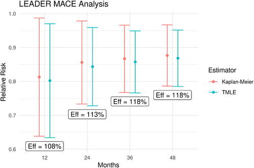
In our application, the estimated risks of MACE, $1-\widehat{S_0}(t)$, in the above denominators increase over time and the growing denominators overshadow the growing variances of the survival estimates, resulting in the shrinking variances for our relative risk estimators over time. While the true parameter value in this case is unknown, thus, precluding comparisons of estimator bias, MSE or confidence interval coverage; we do see the expected efficiency gains of TMLE over Kaplan-Meier of 7 to 18%. This modest precision improvement may be expected as baseline covariates rarely remain highly predictive of outcomes occurring multiple years in the future. When compared to the Cox HR estimator, TMLE estimates of the relative risks of MACE also show up to 13% reduction in 95% confidence interval width for the Year 4 relative risk compared to that of the Cox HR. We focus here and in the subsequent section on the Year 4 relative risks to allow the estimators comparable access to data, as Cox averages across all of the observed data whereas Kaplan-Meier and TMLE use only the events occurring at or before the targeted time.

8.2 Subgroup Analysis

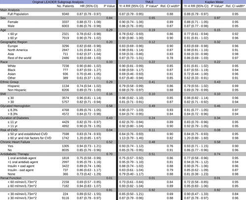
In the original LEADER analysis, Cox regressions were performed for each of 33 subgroups with respect to the primary outcome, MACE, and p-values for between-group differences were reported without adjustment for multiple testing. We performed an analogous subgroup analysis using TMLE and Kaplan-Meier to estimate relative risk of MACE by the end of 12, 24, 36, and 48 months. Figure 5 compares the Kaplan-Meier and TMLE estimates of year 4 relative risk against the primary paper’s Cox HR results. Covariate adjustment set and the candidate hazard learners were the same as for the primary analysis, but prespecified, flexible covariate screening was performed to account for the varying sample sizes of various subgroups. Covariates were ranked according to their Pearson correlation coefficient with respect to the time-to-event and screening was set to the top 15, 40, or 60 covariates based on subgroup sample size cutoffs of less than 500, 1000, 1500 subjects, respectively. No covariate screening was done for subgroups containing more than 1500 subjects. In all 33 subgroups, TMLE with Super Learner returned a point estimate of the effect similar to Cox HR, which again we might expect given the low incidence of MACE in LEADER and seemingly proportional hazards. On the other hand, the TMLE estimate of the year four relative risk was more precise than the Cox HR estimate across all subgroups (up to a 26% relative reduction in 95% confidence interval width), while also showing precision gains relative to Kaplan-Meier.

Figure 5: Primary and Subgroup LEADER Analysis: Treatment effects are summarized by a hazard ratio in the original LEADER analyses (left) and by relative cumulative risk at four years estimated using TMLE (middle) and Kaplan Meier (right). p-values from Welch’s t-test and Welch’s ANOVA are reported without adjustment for multiple testing. Relative 95% CI widths are reported with respect to the confidence interval of the unadjusted Cox HR.

9 Discussion

In this article we echoed concerns regarding the use of Cox HR-based analysis for time-to-event RCTs; in light of the advances in our understanding of causal inference and in the development of estimators for survival estimands, continued adherence to the Cox HR as a survival estimand is becoming increasingly indefensible. We argued for a principled alternative to Cox in the form of a causal roadmap using targeted learning to estimate a survival curve derived estimand and then applied the three part process; (a) defining a causal target quantity in terms of an ideal experiment, (b) establishing the necessary conditions for identifying the causal target with a statistical estimand defined by the observed data, and (c) estimating the target statistical quantity using a prespecified statistical approach that provides robust and efficient inference; to a hypothetical RCT data structure with a right-censored time-to-event outcome. Though nontrivial, adhering to this process will provide researchers with clear benefits: an interpretable and well-defined statistical estimand, with clearly stated assumptions under which this estimand identifies their true causal quantity of interest. In simulations we demonstrated the double robustness and efficiency properties of TMLE, showing the ability of a TMLE using Super Learner for initial estimates to correct for model misspecification and informative censoring. The simulations also showed the finite sample precision gains offered by TMLE relative to Kaplan-Meier. Our parallel reanalysis of LEADER trial data then reassuringly demonstrated that a TMLE targeting relative risk when compared to Cox provides compatible but more precise estimates of treatment effects, even in a setting where Cox is expected to perform well. In fact, TMLE did so not only for the primary analysis, but also across all 33 subgroup analyses. Though this result is expected from theory, here we have shown in real data that treatment effect estimation using TMLE carries little risk when Cox assumptions are plausible, while providing substantial improvement when those assumptions are not plausibly met. Using Super Learner to flexibly adjust for informative censoring reinforces prespecified TMLE analysis plans against unexpected and potentially informative subject dropout; meanwhile flexible adjustment in estimating event hazards provides the opportunity for researchers and clinicians to posit a variety of dependencies and covariate interactions, all while allowing the data to select a model that best captures the actual underlying data-generating process. In practice, the potential efficiency gains offered by TMLE translates to the possibility to achieve desired levels of power with shorter and smaller trials, and can enhance the ability of trials to detect treatment effects in underrepresented subject subgroups. We suggest that more widespread adoption of this targeted learning approach would improve the relevance of survival RCTs for protecting patient safety and improving health.

Acknowledgments

We are grateful for the help of our colleagues in the “Joint Initiative for Causal Inference” from UC Berkeley, University of Copenhagen, and Novo Nordisk; this article has benefited greatly from their broad input.

Disclosure Statement

The authors report no competing interests to declare.

Additional information

Funding

The author(s) disclosed receipt of the following financial support for the research, authorship, and/or publication of this article: This work was supported by a Research Gift from Novo Nordisk. The authors gratefully acknowledge Novo Nordisk A/S.

References

- Aalen, O. O., Cook, R. J., and Røysland, K. (2015), “Does Cox Analysis of a Randomized Survival Study Yield a Causal Treatment Effect?” Lifetime Data Analysis, 21, 579–593. DOI: 10.1007/s10985-015-9335-y.
- Administration UFaD. (2008), “Guidance for Industry Diabetes Mellitus — Evaluating Cardiovascular Risk in New Antidiabetic Therapies to Treat Type 2 Diabetes.”
- Administration UFaD (2018), “Meeting of the Endocrinologic and Metabolic Drugs Advisory Committee Meeting Announcement,” October 24–25, 2018.
- Administration UFaD (2020), “Type 2 Diabetes Mellitus: Evaluating the Safety of New Drugs for Improving Glycemic Control: Guidance for Industry.”
- American Diabetes Association (2020), “10. Cardiovascular Disease and Risk Management: Standards of Medical Care in Diabetes-2020,” Diabetes Care, 43, S111–S134.
- Benkeser, D., and van der Laan, M. J. (2016), “The Highly Adaptive Lasso Estimator,” in 2016 IEEE International Conference on Data Science and Advanced Analytics (DSAA), pp. 689–696. DOI: 10.1109/DSAA.2016.93.
- Benkeser, D., Carone, M., and Gilbert, P. B. (2018), “Improved Estimation of the Cumulative Incidence of Rare Outcomes,” Statistics in Medicine, 37, 280–293. DOI: 10.1002/sim.7337.
- Benkeser, D., Díaz, I., Luedtke, A., and Segal, J., Scharfstein, D., and Rosenblum, M. (2020), “Improving Precision and Power in Randomized Trials for COVID-19 Treatments Using Covariate Adjustment, for Binary, Ordinal, and Time-to-Event Outcomes,” Biometrics, 77, 1467–1481. DOI: 10.1111/biom.13377.
- Bibaut, A. F., and van der Laan, M. J. (2019), “Fast Rates for Empirical Risk Minimization over càdlág Functions with Bounded Sectional Variation Norm,” arXiv:1907.09244 [math, stat]. version: 2.
- Bickel, P. J., Klaassen, C. A. J., Ritov, Y., and Wellner, J. A. (1998), Efficient and Adaptive Estimation for Semiparametric Models, New York: Springer-Verlag.
- Cai, W., and van der Laan, M. J. (2020), “One-Step Targeted Maximum Likelihood Estimation for Time-to-Event Outcomes,” Biometrics, 76, 722–733. DOI: 10.1111/biom.13172.
- Cochran, W. G., and Rubin, D. B. (1973), “Controlling Bias in Observational Studies: A Review,” Sankhyā: The Indian Journal of Statistics, Series A (1961–2002), 35, 417–446.
- Cox, D. R. (1972), “Regression Models and Life-Tables,” Journal of the Royal Statistical Society, Series B, 34, 187–220. DOI: 10.1111/j.2517-6161.1972.tb00899.x.
- Daniel, R., Zhang, J., and Farewell, D. (2021), “Making Apples from Oranges: Comparing Noncollapsible Effect Estimators and their Standard Errors after Adjustment for Different Covariate Sets,” Biometrical Journal, 63, 528–557. Available at DOI: 10.1002/bimj.201900297.
- Didelez, V., and Stensrud, M. J. (2022), “On the Logic of Collapsibility for Causal Effect Measures,” Biometrical Journal, 64, 235–242. Available at DOI: 10.1002/bimj.202000305.
- Efron, B. (1988), “Logistic Regression, Survival Analysis, and the Kaplan-Meier Curve,” Journal of the American Statistical Association, 83, 414–425. DOI: 10.1080/01621459.1988.10478612.
- Gill, R. D., van der Laan, M. J., and Robins, J. M. (1997), “Coarsening at Random: Characterizations, Conjectures, Counter-Examples,” in: Proceedings of the First Seattle Symposium in Biostatistics. Lecture Notes in Statistics, eds. D. Y. Lin and T. R. Fleming, pp. 255–294, New York: Springer. DOI: 10.1007/978-1-4684-6316-3_14.
- Greenwood, M. (1926), The Natural Duration of Cancer. Reports of Public Health and Related Subjects 1926 (no. 33), pp. 1–26, London: Her Majesty’s Stationery Office.
- Heitjan, D. F., and Rubin, D. B. (1991), “Ignorability and Coarse Data,” Annals of Statistics, 19, 2244–2253.
- Hernán, M. A. (2010), “The Hazards of Hazard Ratios,” Epidemiology (Cambridge, Mass.), 21, 13–15. DOI: 10.1097/EDE.0b013e3181c1ea43.
- Hernán, M. A., Hernández-Díaz, S., and Robins, J. M. (2004), “A Structural Approach to Selection Bias,” Epidemiology, 15, 615–625. DOI: 10.1097/01.ede.0000135174.63482.43.
- Ishwaran, H., Kogalur, U. B., Blackstone, E. H., and Lauer, M. S. (2008), “Random Survival Forests,” The Annals of Applied Statistics, 2, 841–860. DOI: 10.1214/08-AOAS169.
- Jacobsen, M., and Keiding, N. (1995), “Coarsening at Random in General Sample Spaces and Random Censoring in Continuous Time,” Annals of Statistics, 23, 774–786.
- Jewell, N. P. (2003), Statistics for Epidemiology (1st ed.), p. 25, Boca Raton, FL: Routledge.
- Lin, R. S., Lin, J., Roychoudhury, S., Anderson, K. M., Hu, T., Huang, B., et al. “Alternative Analysis Methods for Time to Event Endpoints Under Nonproportional Hazards: A Comparative Analysis. Statistics in Biopharmaceutical Research 12, 187–198. DOI: 10.1080/19466315.2019.1697738:187–98.
- Marso, S. P., Daniels, G. H., Brown-Frandsen, K., Kristensen, P., Mann, J. F. E., Nauck, M. A., et al. (2016), “Liraglutide and Cardiovascular Outcomes in Type 2 Diabetes,” New England Journal of Medicine, 375, 311–322. DOI: 10.1056/NEJMoa1603827.
- Martinussen, T., Vansteelandt, S., and Andersen, P. K. (2018), “Subtleties in the Interpretation of Hazard Ratios,” arXiv:1810.09192 [math, stat].
- Moore, K. L., and van der Laan, M. J. (2009a), “Covariate Adjustment in Randomized Trials with Binary Outcomes: Targeted Maximum Likelihood Estimation,” Statistics in Medicine, 28, 39–64. DOI: 10.1002/sim.3445.
- Moore, K. L., and van der Laan, M. J. (2009b), “Increasing Power in Randomized Trials with Right Censored Outcomes Through Covariate Adjustment,” Journal of Biopharmaceutical Statistics, 19, 1099–1131.
- Neyman, J., Dabrowska, D. M., and Speed, T. P. (1990), “On the Application of Probability Theory to Agricultural Experiments. Essay on Principles. Section 9,” Statistical Science, 5, 465–472. DOI: 10.1214/ss/1177012031.
- Pearl, J. (2000), Causality: Models, Reasoning, and Inference (1st ed.), 400 pp., Cambridge, UK; New York: Cambridge University Press.
- Pearl, J. (2009), “Causal Inference in Statistics: An Overview,” Statistics Surveys, 3, 96–146.
- Pearl, J. (2010), “On the Consistency Rule in Causal Inference: Axiom, Definition, Assumption, or Theorem?” Epidemiology, 21, 872–875.
- Pearl, J., Glymour, M., and Jewell, N. P. (2016), Causal Inference in Statistics - A Primer (1st ed.), 156 pp., Chichester: Wiley.
- Petersen, M. L., and van der Laan, M. J. (2014), “Causal Models and Learning from Data: Integrating Causal Modeling and Statistical Estimation,” Epidemiology (Cambridge, Mass.) 25, 418–426. DOI: 10.1097/EDE.0000000000000078.
- Petersen, M. L., Porter, K. E., Gruber, S., Wang, Y., and van der Laan, M. J. (2012), “Diagnosing and Responding to Violations in the Positivity Assumption,” Statistical Methods in Medical Research, 21, 31–54. DOI: 10.1177/0962280210386207.
- Robins, J. (1986), “A New Approach to Causal Inference in Mortality Studies with a Sustained Exposure Period–Application to Control of the Healthy Worker Survivor Effect,” Mathematical Modelling, 7, 1393–1512. DOI: 10.1016/0270-0255(86)90088-6.
- Robins, J. (1999), “Robust Estimation in Sequentially Ignorable Missing Data and Causal Inference Models,” in Proceedings of the American Statistical Association: Section on Bayesian Statistical Science, pp. 6–10, Alexandria, VA.
- Robins, J. M., and Rotnitzky, A. (1992), “Recovery of Information and Adjustment for Dependent Censoring Using Surrogate Markers,” in AIDS Epidemiology: Methodological Issues, eds. N. P. Jewell, K. Dietz, and V. T. Farewell, pp. 297–331, Boston, MA: Birkhäuser.
- Rubin, D. B. (1974), “Estimating Causal Effects of Treatments in Randomized and Nonrandomized Studies,” Journal of Educational Psychology, 66, 688–701. DOI: 10.1037/h0037350.
- Rytgaard, H. C. W., Eriksson, F., and van der Laan, M. J. (2021), “Estimation of Time-Specific Intervention Effects on Continuously Distributed Time-to-Event Outcomes by Targeted Maximum Likelihood Estimation,” arXiv:2106.11009 [stat].
- Simon, N., Friedman, J., Hastie, T., and Tibshirani, R. (2011), “Regularization Paths for Cox’s Proportional Hazards Model via Coordinate Descent,” Journal of Statistical Software, 39, 1–13. DOI: 10.18637/jss.v039.i05.
- Sparapani, R. A., Logan, B. R., McCulloch, R. E., and Laud, P. W. (2016), “Nonparametric Survival Analysis using Bayesian Additive Regression Trees (BART),” Statistics in Medicine, 35, 2741–2753. DOI: 10.1002/sim.6893.
- Stensrud, M. J., Aalen, J. M., Aalen, O. O., and Valberg, M. (2019), “Limitations of Hazard Ratios in Clinical Trials,” European Heart Journal, 40, 1378–1383. DOI: 10.1093/eurheartj/ehy770.
- Stensrud, M. J., Valberg, M., Røysland, K., and Aalen, O. O. (2017),“Exploring Selection Bias by Causal Frailty Models: The Magnitude Matters,” Epidemiology, (Cambridge, Mass.), 28, 379–386. DOI: 10.1097/EDE.0000000000000621.
- Stitelman, O. M., De Gruttola, V., and van der Laan, M. J. (2012), “A General Implementation of TMLE for Longitudinal Data Applied to Causal Inference in Survival Analysis,” The International Journal of Biostatistics, 8. DOI: 10.1515/1557-4679.1334.
- Stitelman, O. M., Wester, C. W., De Gruttola, V., and van der Laan, M. J. (2011), “Targeted Maximum Likelihood Estimation of Effect Modification Parameters in Survival Analysis,” The International Journal of Biostatistics, 7, 19. DOI: 10.2202/1557-4679.1307.
- Uno, H., Claggett, B., Tian, L., Inoue, E., Gallo, P., Miyata, T., et al. (2014), “Moving Beyond the Hazard Ratio in Quantifying the Between-Group Difference in Survival Analysis,” Journal of Clinical Oncology, 32, 2380–2385. DOI: 10.1200/JCO.2014.55.2208.
- Uno, H., Wittes, J., Fu, H., Solomon, S. D., Claggett, B., Tian, L., et al. (2015), “Alternatives to Hazard Ratios for Comparing Efficacy or Safety of Therapies in Noninferiority Studies,” Annals of Internal Medicine, 163, 127–134. DOI: 10.7326/M14-1741.
- van der Laan, M. J. (2017), “A Generally Efficient Targeted Minimum Loss Based Estimator based on the Highly Adaptive Lasso,” The International Journal of Biostatistics, 13. DOI: 10.1515/ijb-2015-0097.
- van der Laan, M. J., Hubbard, A. E., and Robins, J. M. (2002), “Locally Efficient Estimation of a Multivariate Survival Function in Longitudinal Studies,” Journal of the American Statistical Association, 97, 494–507. DOI: 10.1198/016214502760047023:494–507.
- van der Laan, M. J., Polley, E. C., and Hubbard, A. E. (2007), “Super Learner,” Statistical Applications in Genetics and Molecular Biology, 6. DOI: 10.2202/1544-6115.1309.
- van der Laan, M. J., and Robins, J. M. (2003), Unified Methods for Censored Longitudinal Data and Causality. Springer Series in Statistics. New York: Springer-Verlag.
- van der Laan, M. J., and Rose, S. (2011), Targeted Learning: Causal Inference for Observational and Experimental Data. Springer Series in Statistics. New York: Springer-Verlag. DOI: 10.1007/978-1-4419-9782-1.
- van der Laan, M. J., and Rose, S. (2018), Targeted Learning in Data Science: Causal Inference for Complex Longitudinal Studies. Springer Series in Statistics. Cham: Springer. DOI: 10.1007/978-3-319-65304-4.
- van der Laan, M. J., and Rubin, D. (2006), “Targeted Maximum Likelihood Learning,” The International Journal of Biostatistics, 2. DOI: 10.2202/1557-4679.1043.