Bayesian and Frequentist Approaches to Rescuing Disrupted Trials: A Report from the NISS Ingram Olkin Forum Series on Unplanned Clinical Trial Disruptions

Abstract

The COVID-19 pandemic impacted clinical trials in ways never expected. However, similar challenges should now be expected going forward. These challenges made us aware of statistical problems arising from other types of disruptions that had not previously captured the attention of the statistical community. This article describes some frequentist and Bayesian statistical tools that can be used with future disruptions and illuminates issues that could benefit from more statistical research. Disruptions may threaten a clinical trial’s validity. Here, we address two resultant challenges: (a) performing an unplanned analysis with options to stop and/or change the sample size; and (b) changes in the study population that are observable or unobservable at the patient level. Different paradigms lead to different ways of doing things, but many statisticians work exclusively within a Bayesian or frequentist paradigm. We propose and provide side-by-side descriptions of Bayesian and frequentist approaches to dealing with these challenges. An illustrative phase III trial aims to compare second-line therapies for type 2 diabetes. We compare and contrast Bayesian and frequentist coping strategies assuming the trial was interrupted due to COVID-19, focusing on Type I error control and the expected loss from a specific utility function.

Keywords:

• Decision-theoretic designs
• Flexible designs
• Informative interim adaptations
• Population changes
• Sample size re-estimation

1 Introduction

Disruptions of a clinical trial due to extenuating circumstances are defined in Orkin et al. (2021) as unavoidable situations that prompt modifications to a trial. The advent of the COVID-19 pandemic in early 2020 halted recruitment to trials, interfered with treatment regimens, and postponed or modified patient assessments. In many cases, exposure to COVID-19 led to changes in the patient population and required reassessment of study objectives. The validity of a clinical trial may be threatened by such disruptions. We provide guidance for meeting challenges arising from disrupted phase III clinical trials.

A simple example of a study of treatments for type 2 diabetes is introduced in Section 2 along with descriptions of planned Bayesian and frequentist designs and analyses. Section 3 describes frequentist rules for unplanned interim design changes, while Section 4 discusses Bayesian approaches. Section 5 compares these approaches in the context of our diabetes example. Section 6 considers how to accommodate changes to the underlying population. We conclude in Section 7 with a summary of our findings and suggestions for future work. Supplementary materials lists the R code files for computations, simulations and figures which are provided in a zip file. A table showing notation is included in the supplementary material which also includes an overview of Bayesian methods and the likelihood principle.

This article is the product of a working group formed from Session 6 of the National Institute of Statistical Sciences (NISS) Ingram Olkin Forum Series on Unplanned Clinical Trial Disruptions held on April 27, 2021. For more information on this scholarly activity click here.

2 A Clinical Trial Example—A Diabetes Study

2.1 Statistical Model

We consider a hypothetical clinical trial to compare the effect of metformin combined with a new drug versus metformin plus sulfonylurea as second-line therapies for diabetes patients for whom first-line treatment with metformin no longer controls the patient’s HbA1c, a measure of glycated hemoglobin in the blood. The primary outcome is defined as the six-month change in HbA1c from baseline.

Let μ_j represent the mean six-month change from baseline in HbA1c for metformin plus sulfonylurea (j = 0) and for metformin plus the new agent (j = 1). For simplicity, we use mean six-month change from baseline to highlight the issues regarding inference on the treatment effect without adding extra notation for covariates, although in practice, the most efficient design is ANCOVA with baseline HbA1c as a covariate (Vickers 2001; Colantuoni and Rosenblum 2015; Khunti et al. 2018, Appendix B.1 in the supplementary material).

Suppose the trial recruits 2m patients and randomizes these equally to the control arm and the new treatment arm. The observed six-month changes in HbA1c are $y_{\mathit{\text{ij}}}\sim N({\mu }_j,{\sigma }^2)$, $i=1,\dots ,m$; $j=0,1$. We assume σ is known with ${\sigma }^2=0.95$. The treatment effect is $\delta ={\mu }_1-{\mu }_0$. The changes y_ij are calculated as (Baseline - 6-month), so positive values of δ indicate greater reduction in HbA1c with metformin plus the new agent. At the end of the study, we will recommend metformin + ‘new drug’ if we reject the (one-sided) null hypothesis.

2.2 An Initial Frequentist Approach

In the frequentist setting, the decision taken at the end of the study is commonly based on a hypothesis test. Let H₀ denote the null hypothesis that $\delta \le 0$. Conventionally, the decision is taken to recommend the new drug if this (one-sided) null hypothesis is rejected at the α level.

An estimate of the treatment effect $\widehat{\delta }$ is the difference between the two treatment groups of the mean six-month change in HbA1c, ${\overline{Y}}_1-{\overline{Y}}_0$, with variance $\mathit{\text{Var}}(\widehat{\delta })$. The decision rule is then to recommend the new treatment if $\widehat{\delta }$ is sufficiently large, say $Z\ge k$, where $Z=\widehat{\delta }/\surd \{\mathit{\text{Var}}(\widehat{\delta })\}$ so that $Z\sim N(0,1)$ under H₀, and $k={\Phi }^{-1}(1-\alpha )$ to give a one-sided Type I error rate of α.

Suppose randomization is 1:1 and power $1-\beta$ is required under a specified effect size δ_alt, that is, the probability of rejecting H₀ should be $1-\beta$ if $\delta ={\delta }_{\mathit{\text{alt}}}$. Then, the required sample size per group is (1) $$m=\frac{2{\sigma }^2{(z_{1-\alpha }+z_{1-\beta })}^2}{{\delta }_{\mathit{\text{alt}}}^2}.$$(1)

For $1-\beta =0.9$, $\alpha =0.025$, ${\delta }_{\mathit{\text{alt}}}=0.2$ and ${\sigma }^2=0.95$, 500 patients per group are needed.

This design does not include interim analyses, so as not to conflate issues that come with unplanned disruptions. Although we focus on procedures that have parametric assumptions, randomization tests could be used to control Type I error without parametric assumptions. Their role in clinical trials with unplanned disruptions is described in a working paper by Diane Uscher, Alex Sverdlov, Kerstine Carter, Jonathan Chipman, Olga Kuznetsova, Jone Renteria, Victoria Johnson, Chris Barker, Nancy Geller, Michael Proschan, Martin Posch, Sergey Tarima, Frank Bretz and William F. Rosenberger.

2.3 Initial Bayesian Approaches

There are different ways one can apply Bayesian inferential ideas to the design of clinical trials. Appendix B.2 in the supplementary material provides an overview of Bayesian approaches. We consider two Bayesian designs: The first chooses the new treatment if the posterior probability that the treatment effect exceeds a prespecified amount is greater than some threshold, say, 95%, at the time of the analysis, and the second design uses a decision-theoretic approach that incorporates a utility function. Both designs are simple Bayesian designs without interim analyses as in the frequentist design of Section 2.2 to simplify comparisons of these approaches after the onset of disruptions (see Section 5), even though many Bayesian and frequentist designs incorporate interim looks at the data.

2.3.1 A Design Based on a Bayesian Posterior Distribution

Suppose the prior distribution for the treatment effect is $\delta \sim N({\nu }_0,{\tau }_0^2)$. Then $\widehat{\delta }|\delta \sim N(\delta ,2{\sigma }^2/m)$, and the posterior distribution is $\delta |\widehat{\delta }\sim N({\delta }_{\text{post}},{\tau }_{\text{post}}^2)$, where $$\begin{array}{c}{\tau }_{\text{post}}^2={\{1/{\tau }_0^2+m/(2{\sigma }^2)\}}^{-1}\hspace{1em}\text{and}\\ {\delta }_{\text{post}}={\tau }_{\text{post}}^2[{\nu }_0/{\tau }_0^2+m\widehat{\delta }/(2{\sigma }^2)].\end{array}$$

Following observation of data, a decision in favor of the new treatment may be made if the posterior probability that the treatment difference is larger than a certain pre-specified amount exceeds some threshold. Posterior probability thresholds for decision making or the values of hyperparameters in the prior distributions may then be set to provide operating characteristics that align with typical frequentist designs’ error probabilities. Little (2006) calls such designs stylized Bayes or calibrated Bayes. In our working example, we will conclude that the new treatment is better than the control if the posterior probability that $\delta >0$ is greater than or equal to 0.95.

The choice of a prior distribution is discussed in Appendix B.4 in the supplementary material. One possibility is to use a skeptical prior distribution that places most of the probability around no treatment difference, reflecting a prior belief that the new treatment is not superior to the control. As data accumulate, the likelihood will dominate, and the posterior distribution will shift in favor of values supported by the data.

It is convenient to express the prior variance for δ relative to the (assumed known) data variance as ${\sigma }_{\text{skep}}^2={\sigma }^2/n_{0,\text{skep}}$ for this skeptical prior distribution. One may think of this formulation of the prior variance as a posterior distribution of δ from an independent sample of $n_{0,\text{skep}}$ individuals.

The example (Section 2.2) sets a target sample size of 1000 patients to achieve 90% power for a treatment difference $\delta =0.2$ with a one-sided 0.025-level test. If the skeptic believes that $\mathrm{\text{Pr}}(\delta \ge 0.2)=\gamma$, for some small γ ($0\le \gamma \le 1$), then we can solve for $n_{0,\text{skep}}$ with the skeptical prior $\delta \sim N(0,{\sigma }^2/n_{0,\text{skep}})$. We calibrate the decision rule “Decide in favor of H₁: $\delta >0$ if the skeptic’s posterior ${\text{Pr}}_{\text{skep}}(\delta >0.0|\text{Data})>0.95$ at the end of the study” to correspond (roughly) to these frequentist error probabilities. A little algebra shows that $n_{0,\text{skep}}/(2m)=z_{1-\gamma }^2/4{(z_{1-\alpha }+z_{1-\beta })}^2.$ If, for example, $\gamma =0.05$, then the prior sample size for the skeptic is 0.1287 times the sample size per group or $n_{0,\text{skep}}=64.4$. Figure 1(a) shows the prior and posterior densities when the sample estimate $\widehat{\delta }$ is 0 and Figure 1(b) shows these densities when $\widehat{\delta }$ is 0.2. (The R code for simulating the diabetes data and creating Figure 1(a) and (b) is in the files “GenerateDiabetesData.R” and “PlotsForPaper.R”, respectively, in the supplementary material.)

Fig. 1 Prior and posterior distributions for the skeptic under two different scenarios. The data (likelihood) dominate the posterior inference in this example clinical trial.

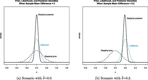
Estimates of operating characteristics based on 10,000 simulations show that with this prior specification (assuming the variance is known), the frequentist operating characteristics roughly match the example study. Simulating data with δ = 0 shows that the skeptic’s posterior probability $${\text{Pr}}_{\text{skep}}(\delta >0.0|\text{Data})>0.95$$ occurred around 3.2% of the time. When generating data with $\delta =0.2$, the decision in favor of the new treatment based on ${\text{Pr}}_{\text{skep}}(\delta >0.0|\text{Data})>0.95$ occurred 92.2% of the time. (This R code is in the file “CalibratedPriorBayesianDesign.R” in the supplementary material.)

2.3.2 A Bayesian Decision-Theoretic Design

A Bayesian decision-theoretic design requires specification of a utility function that reflects the needs and goals of the study. The optimal study design is the one that maximizes the expected utility. We base our utility function on the one in Berry and Ho (1988).

Suppose that the potential gain from choosing the new treatment over the control is proportional to the treatment effect, δ. This gain would be realized if one correctly concludes that the study treatment is better than the control. Although one could posit a future loss that is proportional to the relative inferiority of the new treatment, we assume a constant loss.

If the decision is to recommend the new treatment, our utility (future “loss”) is $$L(\delta )=\{\begin{array}{cc}-B(\delta -{\delta }_0)& \text{if}\delta >{\delta }_0\\ L& \text{if}\delta \le {\delta }_0,\end{array}$$ and zero otherwise. Here B > 0 is the benefit, L > 0 is the constant loss, and δ₀ is 0 or a minimal improvement that one wants to see. As shown in eq. (3.4) on p. 222 of Berry and Ho (1988), if the new treatment is recommended at the end of the trial, the expected risk as a function of the posterior of δ is (2) $$R({\delta }_{\text{post}})=L\Phi (s)-B{\tau }_{\text{post}}\left\{\varphi (s)-s\left[1-\Phi (s)\right]\right\},$$(2) and the risk is zero if the new treatment is not recommended. Here, $\Phi (·)$ is the cdf of the standard normal function, $\varphi (·)$ is the pdf of the standard normal, ${\delta }_{\text{post}}$ is the posterior mean of δ, ${\tau }_{\text{post}}$ is the posterior standard deviation, and $s=-{\delta }_{\text{post}}/{\tau }_{\text{post}}$ (see Appendix C.2 in the supplementary material).

We consider L and B to be in the same units, without loss of generality, expressed in units per patient, as in Berry and Ho (1988). The sample size does not appear explicitly in the risk function given by equation (2)(2) $$R({\delta }_{\text{post}})=L\Phi (s)-B{\tau }_{\text{post}}\left\{\varphi (s)-s\left[1-\Phi (s)\right]\right\},$$(2) , because the utility function consists of future gain and loss after the trial when one decides in favor of or against the new treatment. At the end of the trial, the cost of the current study has already been spent. Any application of (2) to interim decision making will reflect the decision to continue the study to its pre-planned conclusion and the cost of continuing.

Since our initial design did not include interim analyses, we do not use dynamic programming to determine the optimal sequential decision. Instead, we calibrate the design parameters to make our Bayesian decision-theoretic design’s operating characteristics match those of the frequentist design in our example. As shown in Berry and Ho (1988), (2) gives the expected utility at the end of the study relating to the decision to conclude that the new treatment combination is better than the control.

Assuming the skeptic’s prior, empirically we found that $B=\mathit{\text{cL}}=0.415L$ provides a rejection threshold that leads to a risk of 2.5% of falsely rejecting the null hypothesis of no treatment difference, assuming a known variance in the data equal to 0.95. The probability of correctly declaring that the new treatment is better is 0.90. (This R code is in the file “BayesianDecisionTheoreticDesign_ForPaper.R” in the supplementary material.)

3 Frequentist Rules for Changing the Design

The distribution of the end-of-study estimated effect size depends on if and how pre-disruption data is used in procedures for deciding to terminate a study or recalculate the sample size use at the time of a disruption. We briefly discuss design changes that do not use pre-disruption data in Section 3.1. In Sections 3.2.1 and 3.2.2, we pre-specify how decisions will depend on the pre-disruption analysis; in this case, the probabilities of modification under various scenarios can be calculated. At the end of the study, these known probabilities can be used to obtain the joint distribution of the pre-disruption data and the post-disruption data (if the study continued). Section 3.2.1 shows how to develop a most powerful end-of-study test ($H_0:\delta =0$) given an (exemplary) pre-specified sample size recalculation procedure. Section 3.2.2 describes how a test of $H_0:\delta =0$ can be introduced at the time of disruption that has the desired Type I error rate and maximum power whether or not the study stops or continues.

The popular combination test does not use the sampling distribution of the final summary test statistic (Section 3.2.3). Because the pre- and post-disruption data are combined with fixed weights as independent data, it does not need to specify the decision probabilities at the time of disruption. With the combination test, Type I error rates can be preserved exactly regardless of the way in which the trial design was modified. We also show that the conditional Type I error method (Proschan and Hunsberger 1995) is essentially equivalent. Section 3.3 shows how the combination test applies when the trial design is modified after the pre-disruption response data have been observed.

3.1 Changes to the Study Design That Do Not Use Study Data

We now consider how the trial might be conducted after a disruption has occurred and we elaborate on options to terminate recruitment, pause recruitment, or resume the trial with a new target for the final sample size.

Terminate Recruitment and Perform a Final Data Analysis

Depending on how much of the originally planned data has been collected at the onset of the disruption, we might want to stop the trial and analyze it. The situation can be compared to a trial with more missing data than anticipated. In the case considered here (i.e., circumstances unrelated to the trial), the data is truly missing completely at random (MCAR). Terminating recruitment and analyzing the observed data will control the Type I error rate but yield a smaller power. For trials that have collected nearly all the data, this might be an option assuming the decision to stop the trial is not based on any data other than the amount of data collected so far.

Pause Recruitment with an Option to Restart

When a disruption halts recruitment, one might wish to analyze the data and stop the study if the data observed are not sufficiently promising, otherwise continuing as originally planned to the end of the trial. As stopping for futility cannot lead to rejection of the null hypothesis to claim that the new treatment is effective, introducing a stopping option for futility without changing other design aspects does not inflate the Type I error rate but can slightly reduce power.

It is tempting to analyze the data and stop the trial if the result is significant, and otherwise continue, conducting another analysis when more data is available. However, using the full significance level for both the pre- and post-disruption analyses will lead to Type I error rate inflation (Dmitrienko, D’Agostino Sr., and Huque 2013). To continue the trial after an analysis one needs to formally plan repeated interim analyses in order to control Type I error rates (see Section 3.2.2).

Change the Sample Size

In considering the resumption of a trial following a disruption, one might consider changing the sample size. A decision to change the sample size might be made without using any pre-disruption study data. For example, perhaps external data published on the treatment effect and/or the variance have led to concerns about the planning assumptions. Such a change will not affect the Type I error rate. In an extreme case, the trial might not be resumed because the resulting loss in power is considered unacceptable.

A disruption affecting a trial’s operations might lead to a change in sample size. For example, patients might have missed treatment cycles due to lockdowns and hence receive fewer doses than prescribed, leading to a smaller treatment effect. In this case, an increase in sample size can make up for the expected loss in power.

3.2 Planning Modifications Prior to Looking at Pre-Disruption

In this section, we consider the situation where plans for design modifications based on pre-disruption data are to be made before actually looking at pre-disruption response data. The rules themselves are functions of pre-disruption data, for example, the post-disruption sample size formula could be a function of the estimated effect size, but this function is to be specified before the value of this estimate becomes known.

In Section 3.3, we suppose the team responsible for making design modifications already has knowledge of the pre-disruption results, such as the treatment effect estimate.

3.2.1 Sample Size Recalculation

If one suspects a disruption has led to changes in the response variance ${\sigma }^2$ or the treatment effect δ, it is natural to base design modifications on estimates of ${\sigma }^2$ and δ from the data collected thus far. A key distinction here is whether interim data have been observed by those responsible for making design modifications. If no interim data have been observed, rules for study adaptations may be drawn up as might have been done before the first patient was recruited. Even if the trial monitoring committee has seen interim estimates of ${\sigma }^2$ or δ, the trial steering group, who have not seen such data, may make design modifications and pass on revised rules for study conduct and data analysis to the monitoring committee. However, when response data that allow estimation of ${\sigma }^2$ or δ have been observed by those deciding on study adaptations, protecting the Type I error rate is more challenging.

Using an Interim Estimate of ${\sigma }^2$

Wittes and Brittain (1990) proposed a general framework for updating sample size based on interim estimates of nuisance parameters, such as ${\sigma }^2$ in the normal model: one simply recalculates the sample size using new estimates of these parameters and conducts the final analysis as for a fixed sample size study. Jennison and Turnbull (1999, chap. 14) show this approach can lead to a small amount of Type I error rate inflation when applying a t-test. Friede and Kieser (2003) also note the potential Type I error rate inflation when modifying sample size based on an estimate of ${\sigma }^2$. Kieser and Friede (2003) show that this inflation disappears almost completely if one uses a pooled estimate of the variance, ignoring treatment labels and the possible difference in means of the two treatment groups. Re-estimation of ${\sigma }^2$ does not inflate nominal asymptotic Type I error rates, but power against a fixed alternative tends to 1 asymptotically. Tarima and Flournoy (2019) show that nominal power against a local alternative is realized asymptotically.

It is possible that, in the process of examining data to estimate ${\sigma }^2$, one may learn about the current estimate of δ and we note in the next section that using this to update the sample size can lead to Type I error inflation. In the absence of other information, in the setting of normally distributed data, the use of the pooled estimate of ${\sigma }^2$ to revise the final sample size leads to virtually no inflation of the Type I error rate.

Using an Interim Estimate of δ

Modifying sample size using an estimate of δ poses a greater challenge. In general, changing the final sample size in light of interim data and then conducting a fixed sample size analysis of the resulting data can cause the Type I error rate to be inflated (Proschan et al. 1992), and in extreme cases, more than doubled (Graf and Bauer 2011). The desire for methods that allow sample size increases while protecting the Type I error rate has led to the rapid growth of interest in adaptive designs; see, for example, Cui, Hung, and Wang (1999).

A reason for recalculating the sample size is to have reasonable power at the end of the study over a range of treatment effects. Suppose disruption occurs after $n_1=300$ patients per treatment arm have been observed and let ${\widehat{\delta }}_1$ denote the estimated treatment effect based on responses from these pre-disruption patients. One option is to devise a rule for recalculating the sample size at the interim analysis before observing ${\widehat{\delta }}_1$. We consider two sample size recalculation (SSR) rules, one “Realistic” and one “Expository”, that are defined in terms of fixed ranges of ${\widehat{\delta }}_1$. The modified sample size options in the former are “Realistic” in that they are of the same order of magnitude as the original plan. The “Expository” rule includes the option of using a much larger sample size if the ${\widehat{\delta }}_1$ is very close to the null. We are not promoting the use of any particular rule or sample size reduction. We include these to demonstrate properties under a range of approaches.

The post-disruption sample sizes per treatment arm determined by the “Realistic” and the “Expository” SSR rules are shown in Table 1. The SSR decision is denoted by the random variable D, which takes a value $d\in \{1,2,3,4,5\}$, and this determines the realization n₂ of N₂, the number of patients per treatment arm after the onset of the disruption. Power curves for different test procedures are very similar under the Realistic SSR rule whereas the Expository SSR rule leads to visually different power curves for different testing procedures.

Table 1 Expository and realistic sample size recalculation rules.

	$\text{Pr}(D=d)$	Expository	Realistic
Range for ${\widehat{\delta }}_1$	when δ = 0	SSR rule	SSR rule	Decision D
${\widehat{\delta }}_1\le 0$	0.500	$n_2=0$	$n_2=0$	d = 1, STOP for futility
$0<{\widehat{\delta }}_1\le 0.1$	0.396	$n_2=1000$	$n_2=300$	d = 2, increase sample size
$0.1<{\widehat{\delta }}_1\le 0.2$	0.098	$n_2=200$	$n_2=200$	d = 3, maintain sample size
$0.2<{\widehat{\delta }}_1\le 0.3$	0.006	$n_2=20$	$n_2=100$	d = 4, decrease sample size
${\widehat{\delta }}_1>0.3$	<0.001	$n_2=0$	$n_2=0$	d = 5, STOP for efficacy

NOTE: The value n₂ is a realization of the random post-disruption sample size N₂.

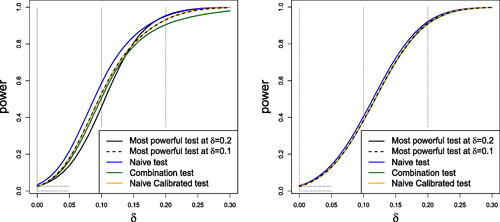
Figure 2 shows the power curve for the end-of-study test under the Expository and Realistic Sample Size Rules using five different hypothesis testing procedures: (a) the most powerful test at $\delta =0.2$ for the given Sample Size Rule, (b) the most powerful test at $\delta =0.1$ for the given Sample Size Rule, (c) the “Naive Test”, (d) the “Combination Test” and (e) the “Naive Calibrated Test”. The Naive test rejects the null hypothesis if the standard Z-statistic based on all the observed data exceeds the standard normal quantile $z_{1-\alpha }$; the Naive Calibrated test uses the same test statistics but with the critical value adjusted so that the overall Type I error is equal to $\alpha =\mathrm{0.025.}$ The Combination Test controls the Type I error probability even when the SSR rule is not pre-specified: see Section 3.2.3 for details. Properties of the most powerful test (that provides the highest possible power at a specific $\delta ={\delta }_{\text{alt}}$ across all α-size tests for a predefined SSR rule) are not standard, and so we elaborate on them before discussing the results in Figure 2 further.

Fig. 2 Power curves under the expository (left) and realistic (right) SSR rules

In the case of the Expository SSR rule: if D = 1, the trial stops for futility and $n_2=0$; if D = 2, the trial continues with $n_2=1000$; if D = 3, then $n_2=200$; if D = 4, then $n_2=20$; if D = 5, the trial stops for efficacy and $n_2=0$. When $n_2>0$, we denote by ${\widehat{\delta }}_2$ the estimate of δ based on n₂ post-disruption observations per treatment arm. For each interim decision $D\in \{2,3,4\}$ and the consequent sample size n₂, the distribution of the Naive test statistic is a convolution of two normal random variables based on n₁ pre-disruption observations and n₂ post-disruption observations per treatment arm. When $D\in \{1,5\},n_2=0$ and the final Z-score is fully determined by the pre-disruption data.

By the Neyman-Pearson Lemma, the likelihood ratio test is the most powerful test between two simple hypotheses $\delta ={\delta }_0$ and $\delta ={\delta }_{\text{alt}}$ (in our example ${\delta }_0=0$), the likelihood ratio $f(\widehat{\delta },d;{\delta }_{\text{alt}})/f(\widehat{\delta },d;{\delta }_0)$ depends on the sufficient statistic $(\widehat{\delta },d)$, where $\widehat{\delta }=[n_1{\widehat{\delta }}_1+n_2(d){\widehat{\delta }}_2(d)]/[n_1+n_2(d)]$. For simplicity, the dependence of n₂ and $\widehat{\delta }$ on the realized interim decision d is suppressed in what follows. If $d\in \{1,5\},{\widehat{\delta }}_2$ is undetermined because n₂ in these two cases is equal to zero; we resolve this uncertainly by setting $n_2{\widehat{\delta }}_2=0$ when $d\in \{1,5\}$. Thus, the sufficient statistic $(\widehat{\delta },d)$ is determined for all sampling combinations. This test rejects the null hypothesis if (3) $$-2(n_1+n_2)\widehat{\delta }({\delta }_0-{\delta }_{\text{alt}})+(n_1+n_2)({\delta }_0^2-{\delta }_{\text{alt}}^2)>k,$$(3) where the critical value k is chosen to give the desired Type I error probability. Since d is the realization of the random variable D, which is a function of ${\widehat{\delta }}_1$, and n₂ is the realization of N₂, the distribution of the test statistic in equation (3)(3) $$-2(n_1+n_2)\widehat{\delta }({\delta }_0-{\delta }_{\text{alt}})+(n_1+n_2)({\delta }_0^2-{\delta }_{\text{alt}}^2)>k,$$(3) is complex. The critical value k may be estimated using Monte Carlo simulations. However, numerically exact computation is also possible. For a given value d of D, and the consequent value n₂ of N₂, the condition (3) can be written as $$Z_d=\surd \{n_1+n_2\}\widehat{\delta }>\frac{k-(n_1+n_2)({\delta }_0^2-{\delta }_{\text{alt}}^2)}{2\surd \{n_1+n_2\}({\delta }_{\text{alt}}-{\delta }_0)}=c_d,$$ say. The probability of observing Z_d > c_d can be calculated using the fact that when $D=d\in \{2,3,4\}$, the distribution of $(n_1+n_2)\widehat{\delta }$ is the convolution of the truncated normal density of $n_1{\widehat{\delta }}_1$ and the normal density of $n_2{\widehat{\delta }}_2$, while for $D=d\in \{1,5\},(n_1+n_2)\widehat{\delta }=n_1{\widehat{\delta }}_1$ is a truncated normal density. Hence, the critical value k can be found by ensuring that the sum of the probabilities $P(Z_d>c_d)$ over $d\in \{1,\dots ,5\}$ is equal to the required Type I error probability α. The resulting test maximizes the power at ${\delta }_{\text{alt}}$ while keeping the overall Type I error at the desired level. Tarima and Flournoy (2022) used a similar approach to finding the most powerful test for a group sequential design which is discussed further in Section 3.2.2.

For each of the five hypothesis testing procedures depicted in Figure 2, sampling terminates with acceptance of H₀ if D = 1 and with rejection of H₀ if D = 5. When $D\in \{2,3,4\}$, the critical value for the Naive and Combination Test Z-statistics is 1.96, whereas in the Naive Calibrated procedure, H₀ is rejected if the Z-statistic is greater than 2.01 in order to achieve a Type I error rate of $\alpha =0.05$. The Most Powerful test at alternative ${\delta }_{\text{alt}}=0.2$ has critical values $c_2=1.84,c_3=1.98$, and $c_4=2.10$, while the Most Powerful test at ${\delta }_{\text{alt}}=0.1$ has $c_2=2.25,c_3=2.10$, and $c_4=2.10$. The R code used to produce the power curves in Figure 2 is available in “LRT_with_SSR.R” in the supplementary material.

Figure 2 shows that, under the Expository SSR rule, the Naive test has the highest power curve of the five tests. However, the Naive test has a Type I error rate of 3.3%, whereas all the other tests secure the desired Type I error rate of 2.5%. The power curve of the Combination Test (the green line) is below that of other tests for $\delta >0.15$. This is because the Combination Test gives fixed weights to ${\widehat{\delta }}_1$ and ${\widehat{\delta }}_2$, and with this rather extreme SSR rule, the sample sizes on which these estimates are based can be very different. When changes from the initially planned sample size are smaller, the Combination Test is very competitive as seen in the power curves for the Realistic SSR rule. In this case, the Combination Test, the Naive Calibrated testing procedure and the two Most Powerful tests have almost identical power curves, while the Naive test has slightly higher power but its Type I error rate is also higher at 2.8%.

3.2.2 Perform a Hypothesis Test and Decide to Continue or Not

It might be desirable to analyze the data before resuming the study with the hope of obtaining a positive result, but continuing the study if this hypothesis test is not significant (without changing the maximum sample size). To plan for multiple testing, we need to pre-specify critical values that ensure control of the Type I error rate before examining the data. Any group-sequential boundaries based on error-spending functions that mimic Pocock (1977) or O’Brien and Fleming (1979) can be used. Depending on the extenuating circumstances and what impact they might have on our trial, one might prefer Pocock-like boundaries over O’Brien-Fleming’s as the probability to stop early with rejection of the null hypothesis is larger. For example, if one believes that data that will be collected after the onset of a disruption differs considerably from the data collected before its start, it might be difficult to interpret the combined data, in which case one would try to maximize the probability of stopping the trial early.

As long as we pre-specify how decisions will depend on the pre-disruption analysis before we look at any of that data, Type I error rates for the end-of-study test of effect size can be controlled. Assuming one knows the sampling distribution of the pre-disruption effect size, the probability of stopping under various scenarios can be calculated. At the end of the study, this known probability of stopping can be used to obtain the joint distribution of the pre-disruption data and the post-disruption data (if the study continued) to create a final test of the effect size as described by Tarima and Flournoy (2022) for two-stage studies with informative stopping rules. For one-parameter exponential families in canonical form, this procedure provides the most powerful test. An application to enrichment designs (Flournoy and Tarima 2023) was developed as an alternative to combination tests proposed by Stallard (2023).

The methods described in Section 3.2.3 avoid using the stopping probability and hence apply to more flexible design modifications, but in the simple testing situation just described they are less powerful.

3.2.3 Methods that Allow Flexibility in Design Modifications

The methods described above assume the SSR rule is specified before pre-disruption data are revealed and, furthermore, they require strict adherence to this rule. If these conditions are met in our example, then the most powerful tests at $\delta =0.1$ and $\delta =0.2$ and the Naive Calibrated test all have Type I error rates equal to 0.025. However, it may be desirable to allow design modifications to depend on additional information in the pre-disruption data and, in that case, another type of testing method is required if the Type I error rate is to be controlled. Two approaches have been proposed to control the Type I error rate when design changes are implemented with some flexibility—but we show that the two proposals can produce essentially the same methods.

Method 1. Combination Tests

One way to create a flexible design and hypothesis test with a given Type I error rate α is to stipulate that a combination test (Bauer and Kohne 1994) will be used to merge summaries of the pre- and post-disruption data. Various combination rules have been proposed but we shall restrict attention to the “inverse normal” combination test. We let n₁ denote the sample size per arm before disruption and N₂ the sample size per arm after the onset of the disruption, using a capital letter as N₂ is a random variable depending on pre-disruption data. Here, estimates ${\widehat{\delta }}_1$ and ${\widehat{\delta }}_2$ based on data before and after the onset of the disruption are used to define standardized statistics $Z_1={\widehat{\delta }}_1\surd \{n_1/(2{\sigma }^2)\}\text{and}{Z}_2={\widehat{\delta }}_2\surd \{N_2/(2{\sigma }^2)\}$ and these are combined in the overall test statistic $Z=w_1{Z}_1+w_2{Z}_2,$ where w₁ and w₂ are constants satisfying $w_1^2+w_2^2=1$. A key point is that w₁ and w₂ are defined before any re-design takes place and they retain their original values regardless of the choice of post-disruption sample size N₂. Under δ = 0, we have $Z_1\sim N(0,1)$, and the conditional distribution of Z₂ is N(0, 1), given the pre-disruption data and any other information that led to the chosen value of N₂. Since the conditional distribution of Z₂ is the same for all values of Z₁ it follows that when δ = 0, Z₁ and Z₂ are statistically independent and $Z\sim N(0,1)$ marginally, regardless of how N₂ is determined. This independence property only holds for the special case δ = 0: if $\delta \ne 0$, Z is not normally distributed since the distribution of $N_2=N_2({\widehat{\delta }}_1)$ depends on δ. However, it is just the properties of Z₁ and Z₂ under δ = 0 that are needed to show that the combination test protects the Type I error rate.

If no early stopping is permitted at the onset of disruption (i.e., $N_2>0$), then at the final and only test, the null hypothesis $\delta \le 0$ is rejected if $Z\ge z_{1-\alpha }$. If early stopping is permitted, to accept H₀ if $Z_1<c_1$ or to reject H₀ if $Z_1>c_2$ say, standard group sequential calculations can be made to set the critical value of Z so that the overall Type I error rate is α. If $\delta <0$, Z₁ and Z₂ are no longer independent, but a coupling argument can be used to show that $P(\text{Reject}{H}_0)<\alpha$ in this case.

Method 2. Preserving the Conditional Type I Error Probability

Suppose, as in our example, the design for a trial is specified and the plan states that the null hypothesis H₀ will be rejected if the final test statistic Z exceeds $z_{1-\alpha }$. Now suppose that design changes are to be made at an interim point during the trial. Let $Z_1={\widehat{\delta }}_1\surd \{n_1/(2{\sigma }^2)\}$, as before. Proschan and Hunsberger (1995) define the conditional Type I error probability as (4) $$A(z_1)=P_{\delta =0}(Z>z_{1-\alpha }|Z_1=z_1).$$(4)

They note that, if δ = 0, the overall Type I error probability can be expressed as (5) $$\int A(z_1)\varphi (z_1)d{z}_1=\alpha ,$$(5) where $\varphi$ denotes the probability density of a N(0, 1) random variable. If the trial design is modified at the onset of the disruption, Type I error probability α can be maintained by ensuring that the conditional probability of rejecting H₀ remains equal to $A(z_1)$, so the overall Type I error probability is still represented by the left-hand side of equation (5)(5) $$\int A(z_1)\varphi (z_1)d{z}_1=\alpha ,$$(5) and so is equal to α. As an example, if a new post-disruption sample size N₂ per arm is chosen, H₀ should be rejected if $Z_2={\widehat{\delta }}_2\surd \{N_2/(2{\sigma }^2)\}>z_{1-A(z_1)}.$ Proschan and Hunsberger (1995) propose several “conditional type I error” functions $A(z_1)$. However, in our example, the function $A(z_1)$ is determined by the fact that H₀ would be rejected in the original design if $Z>z_{1-\alpha }$ where $$Z=\frac{n_1{\widehat{\delta }}_1+n_2^{*}{\widehat{\delta }}_2}{\sqrt{2{\sigma }^2(n_1+n_2^{*})}}=\sqrt{\frac{n_1}{n_1+n_2^{*}}} Z_1+\sqrt{\frac{n_2^{*}}{n_1+n_2^{*}}} Z_2$$ and $n_2^{*}=m-n_1$ is the fixed value for the post-disruption sample size per treatment arm in the original design. Thus, we see that this method is actually equivalent to using an inverse normal combination test with weights $$\surd \{n_1/(n_1+n_2^{*})\}\hspace{1em}\text{and}\hspace{1em}\surd \{n_2^{*}/(n_1+n_2^{*})\}.$$

3.3 Making Design Modifications After Seeing the Data

Now we consider the situation where design modifications are to be made by investigators who have already seen response data. For clarity, we reiterate the distinction from the case considered previously. In Section 3.2.3 we assumed that the rules for making design modifications were specified before any trial data were revealed. The rules themselves could involve trial data, for example, the post-disruption sample size N₂ could be a function of ${\widehat{\delta }}_1$, but this function was to be specified before the value of ${\widehat{\delta }}_1$ became known. In this Section, we shall suppose the team responsible for making design modifications already has knowledge of pre-disruption results, such as the pre-disruption treatment effect estimate ${\widehat{\delta }}_1$.

The key to making progress here is to argue that, although a combination test or conditional Type I error rate function is not mentioned in the original study plan, the original analysis can be described in such a way. In the context of our example, suppose a trial, originally designed to enroll 500 patients per arm, is paused at the onset of a disruption with 300 patients enrolled on each arm. No patients have been admitted since then, but follow-up has continued so that the 6-month endpoint has been recorded for all 300 patients on each treatment arm. It is now planned to resume the study, possibly with some changes to the design.

Müller and Schäfer (2004) propose the use of methods based on the conditional Type I error rate function. In our example, the conditional Type I error probability equation (4)(4) $$A(z_1)=P_{\delta =0}(Z>z_{1-\alpha }|Z_1=z_1).$$(4) can be calculated using current data and the original decision rule. Then once this conditional probability $A(z_1)$ is known, additional data will be collected and a test of H₀ with Type I error probability $A(z_1)$ conducted based on the new data alone. If this test rejects H₀, then H₀ is rejected in the overall testing procedure.

An alternative route to essentially the same end is to note that, in the original plan, H₀ would be rejected if $$Z=\sqrt{\frac{n_1}{n_1+n_2^{*}}} Z_1+\sqrt{\frac{n_2^{*}}{n_1+n_2^{*}}} Z_2\ge z_{1-\alpha },$$ where Z₁ and Z₂ are standardized statistics based on the data gathered before and after the disruption, respectively, and this has the form of an inverse normal combination test with weights $w_1=\surd \{n_1/(n_1+n_2^{*})\}$ and $w_2=\surd \{n_2^{*}/(n_1+n_2^{*})\}$. Following the principles for applying a combination test in a pre-planned adaptive design, one should calculate Z₁, w₁ and w₂, then continue to obtain a standarized statistic Z₂ based on the new data alone and, at the end of the trial, reject H₀ if $w_1{Z}_1+w_2{Z}_2>z_{1-\alpha }$.

The methods described above explain how data from a modified design will be handled. It remains to decide how the design should be modified. Consideration of power or conditional power of the hypothesis test will lead to a choice of post-disruption sample size that will depend on $\widehat{\delta }$ (and possibly ${\widehat{\sigma }}^2$). Since values of these are known, a rule for what would have been done had other values of ${\widehat{\sigma }}^2$ and $\widehat{\delta }$ been observed is not required.

In calculating a conditional error rate or interpreting the original analysis as a combination test we have assumed that, without disruption, the trial would have run as initially described in the trial’s protocol and, in particular, the target sample size would be reached exactly as planned. If there is evidence of a higher or lower recruitment rate than anticipated, with a potential impact on the final sample size, it would be wise to check the sensitivity of the conditional error rate or the weights in a combination test to assumptions about the final sample size.

The methods in this Section have a limitation in that there is no scope for early stopping to make a positive conclusion in favor of the new treatment. This would require the choice of a group sequential testing boundary and setting this after the value of the test statistic is known is clearly problematic. For all these reasons, we recommend avoiding giving access to pre-disruption data before making any modifications to the form of decision rule to be used in the trial.

Even in the preferable setting of Section 3.2.3, flexible adaptive designs may suffer a loss of power due to the way in which summary statistics are combined (e.g., when weights w₁ and w₂ in a combination test are not aligned with sample sizes n₁ and N₂). Allowing many and different adaptations can affect the acceptability of a trial to regulatory agencies: the Committee for Medicinal Products for Human Use (2007) points out that re-assessing the sample size more than once in a trial might raise concerns about the trial while Evans (2007) addresses the issue of changing endpoints in clinical trials. The desire that adaptations be pre-specified is also reflected in the Food and Drug Administration guideline on adaptive designs (Food and Drug Administration 2019). Of course, the unanticipated nature of a disruption implies that unusual steps may be necessary: a middle path is therefore to use adaptive techniques to solve the major problems of trial design without over-elaborating this process.

4 Bayesian Handling of Disrupted Trials

The Bayesian philosophy allows the prior distribution at the time of design, re-design, or analysis to include information that is independent of the study data. That is, one may incorporate into an analysis new external information not available prior to the start of the study when determining the posterior distribution. Thus, in response to disruption of an ongoing trial, a Bayesian could update the posterior distribution to incorporate outside information about how the disruption, its cause, or its sequelae might affect the study population and/or changes that affect the study team’s ability to resume the study.

Recall our example diabetes trial of Section 2 that planned to enroll 500 patients per arm. Suppose a disruption causes the trial to pause with 300 patients enrolled on each arm; no patients have been admitted since the onset of the disruption, but follow-up has continued. Also suppose the 6-month endpoint has now been recorded for all 300 patients on each treatment. The investigators may feel it prudent to analyze the data currently available. In this section, we consider how disruptions to the Bayesian designs described in Section 2.3 might be handled. While we focus on the calibrated Bayesian designs, the interim analysis approaches discussed here could be applied to any design, with or without a disruption.

4.1 What Happens to the Calibrated Bayesian Design?

Simulations can be done to examine the effect an unplanned analysis has on the risk of a Type I error. If the results of the simulations lead regulators or sponsors to be concerned that the Type I error might be too high, the trial team may consider changing decision thresholds for this or subsequent interim analyses. Note that adding interim tests for futility (i.e., failure to reject the null hypothesis) will not, in general, increase the risk of a Type I error but may reduce power. At the same time, adding interim tests for efficacy (i.e., to reject the null hypothesis) may increase the risk of a Type I error but not the risk of a Type II error.

For an example of a Bayesian approach to interim monitoring, we borrow the ideas of Spiegelhalter, Freedman, and Parmar (1994) and consider priors from two perspectives. In Section 2.3.1, we presented a “skeptical” prior distribution that reflected the belief that the treatment difference is most likely around zero but allowed some small chance that δ exceeds a clinically meaningful threshold. We now also consider a second prior distribution that reflects the belief of an enthusiastic individual who places substantial prior probability on the event that the new treatment achieves a clinically significant improvement over the control. This enthusiastic prior, along with any relevant information external to the study, can be used for decisions regarding futility at the onset of the disruption and any subsequent interim analyses.

As an aid to decision making, we consider the range of possible values for the treatment difference δ a little more closely. One might consider a three-part partition of the range of possible δs. One region would correspond to values of δ that clearly indicate superiority of the new treatment by at least a minimally meaningful amount. Another region contains all values of δ that show that the new treatment is probably not worth further consideration. The remaining region may be called a “range of equivalence” (Freedman and Spiegelhalter 1992). If there is a high probability that δ lies in this region, then one would probably want to consider other aspects of the treatment, such as tolerability or cost, before one would recommend it over the control.

In our motivating example, $\delta >0$ favors the new treatment. The region of superiority of the new treatment would be $[{\delta }_{\text{sup}},\infty )$, where ${\delta }_{\text{sup}}$ is the treatment difference that one would think clinically meaningful. This value need not equal the value ${\delta }_{\text{alt}}$ in the frequentist’s alternative hypothesis for which the sample size provides predetermined power. It may well be that $0<{\delta }_{\text{sup}}<{\delta }_{\text{alt}}$. Without loss of generality, in our example we take ${\delta }_{\text{sup}}={\delta }_{\text{alt}}=0.2$. Our skeptic might place more prior probability on the region $(-\infty ,0]$ than on either of the other two regions. The enthusiast, on the other hand, would place more prior probability on $\delta \in (0,\infty )$ than on the complementary region, possibly even 50% probability on $\mathrm{\text{Pr}}(\delta \ge {\delta }_{\text{sup}})$.

Considering that the final analysis will correspond to the posterior probability of δ lying in some range of benefit for the new treatment, the calibrated Bayes design will determine this range and the appropriate probability thresholds for deciding in favor of H₀ or H₁. There are multiple ways that one may determine these tuning parameters for the design. In our example, we sought values that gave the calibrated Bayesian design roughly the same risks of erroneous conclusions under the null and alternative hypotheses. Specifically, a decision in favor of H₁: $\delta >0$ might occur if the skeptic’s ${\text{Pr}}_{\text{skep}}(\delta >0.0|\text{Data})>0.95$ at the end of the study. Similarly, the trial might decide in favor of H₀ if the enthusiast’s posterior probability ${\text{Pr}}_{\text{enth}}(\delta <0.2|\text{Data})$ has high probability.

A corresponding group sequential design might proceed as follows. We presented a skeptical prior $\delta \sim N(0,{\sigma }_{\text{skep}}^2)$ in Section 2.3.1. Similarly, the enthusiastic prior might be centered on the clinically minimal treatment difference with $\delta \sim N(0.2,{\sigma }_{\text{enth}}^2)$.

If the trial resumes, a comparison of the skeptical and enthusiastic posterior distributions at the onset of the disruption and at subsequent analyses could inform interim decisions. With increasing information, the two posterior distributions will get closer to each other. If the skeptic and enthusiast put high posterior probability on $\delta >0$, then the study may decide in favor of the alternative hypothesis. If, on the other hand, the two opinions begin to agree on $\delta \le 0$, then the study may conclude against the new treatment’s superiority. If the two posterior distributions put most of the probability between 0 and a pre-specified clinically important treatment difference, then other considerations will enter the ultimate decision, such as ease of delivery, fewer severe side effects, etc.

This sequential trial’s design should ultimately provide enough information to lead the two hypothetical opinions to more-or-less agree at the end of the study, if not sooner. The determination of the study’s sample size will help achieve that goal. As in Section 2.3.1, we express the prior variances as proportional to the (assumed known) data variance ${\sigma }^2$: ${\sigma }_{\text{skep}}^2={\sigma }^2/n_{0,\text{skep}}$ and ${\sigma }_{\text{enth}}^2={\sigma }^2/n_{0,\text{enth}}$, as if the priors derive from independent samples of $n_{0,\text{skep}}$ and $n_{0,\text{enth}}$ individuals, respectively. What remains is to set the prior variances by selecting the prior “sample sizes” $n_{0,\text{skep}}$ and $n_{0,\text{enth}}$.

In a calibrated Bayes approach, we can set some or all of the prior parameters and/or decision criteria to lead to acceptable frequentist characteristics. Typically, simulations will provide estimates of these frequentist probabilities. The example sets a target sample size of 1000 patients to achieve 90% power for a treatment difference $\delta =0.2$ with a one-sided 0.025-level test [equation (1)(1) $$m=\frac{2{\sigma }^2{(z_{1-\alpha }+z_{1-\beta })}^2}{{\delta }_{\mathit{\text{alt}}}^2}.$$(1) , Section 2.1]. In Section 2.3.1, we determined that $n_{0,\text{skep}}=64.4$, based on the skeptic’s belief that ${\text{Pr}}_{\text{skep}}(\delta \ge 0.2)=\gamma =0.05$.

In similar fashion, if the enthusiast believes a priori that ${\text{Pr}}_{\text{enth}}(\delta <0.0)=0.05$, then $n_{0,\text{enth}}=64.4$. For our example trial with 500 patients per arm, Figure 3(a) shows the prior and posterior densities when the sample estimate $\widehat{\delta }$ at the end of the trial is 0 and Figure 3(b) shows these densities when $\widehat{\delta }$ is 0.2. (The R code for Figure 3(a) and (b) is in the file “PlotsForPaper.R” in the supplementary material.)

Fig. 3 Prior and posterior distributions for the hypothetical skeptic and enthusiast at the end of the planned trial under the null and alternative scenarios. Although the two prior distributions are different, the data lead the two opinions expressed via posterior distributions to converge.

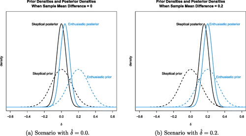
Sensitivity analyses consisting of 10,000 simulations show that with these two prior specifications (assuming the variance is known), the frequentist operating characteristics roughly match the example study. Data generated with δ = 0 show that the skeptic’s posterior probability ${\text{Pr}}_{\text{skep}}(\delta >0.0|\text{Data})>0.95$ occurred in around 3.2% of the simulations, and the enthusiast’s ${\text{Pr}}_{\text{enth}}(\delta <0.2|\text{Data})>0.9$ occurred around 96.5% of the time. The posterior 95% credible interval for δ at this interim analysis is (–0.026, 0.203) using the enthusiastic prior. For reference, the enthusiast’s prior 95% credible interval was (0.032, 0.3683), so there is less enthusiasm now. In this scenario, the skeptic’s skepticism is strongly reinforced, and the enthusiast agrees that $\delta <0.2$. This analysis may lead the study team to stop the trial now for futility.

On the other hand, when data are generated with $\delta =0.2$, the skeptic’s ${\text{Pr}}_{\text{skep}}(\delta >0.0|\text{Data})>0.95$ occurred 92.2% of the time, while the enthusiast’s ${\text{Pr}}_{\text{enth}}(\delta <0.2|\text{Data})>0.9$ only occurred in 7.2% of the simulations. In this scenario, both parties tend to agree that $\delta >0$ with the new treatment.

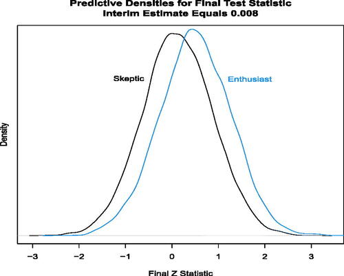
One can also compute the predictive probability that the trial will ultimately conclude at the end of the trial that the new treatment is significantly better, given data at an interim analysis. Suppose that we have full data on 600 (300 per arm) of the planned 1000 patients in our diabetes example. A simulation with δ = 0 yields a mean (standard error) 6-month HbA1c change of–0.070 {0.944/$\surd (300)$} in the control group and–0.078 {0.916/$\surd (300)$} in the group receiving the new treatment. The posterior 95% credible interval for δ at this interim analysis is (–0.065, 0.196) using the enthusiastic prior. For comparison, the enthusiast’s prior 95% credible interval was (–0.038, 0.438), so there is less enthusiasm now. Furthermore, the enthusiast’s predicted probability of ultimately achieving a statistically significant p-value (p < 0.025) is 2.8%. The skeptic’s prediction gives an even smaller probability. This analysis may lead the study team to stop the trial now for futility. (See Appendix B.3 in the supplementary material). Figure 4 shows the skeptic’s and enthusiast’s predictive distributions for the final test statistic ($Z=$ $\widehat{\delta }/\surd \{0.95\times 2/500\}$) as if the trial were to continue to enroll all 1000 patients, given the interim data $\widehat{\delta }$=0.008 at the onset of the disruption. (The R code for Figure 4 is in the file “PlotsForPaper.R” in Section 7 supplementary material.)

Fig. 4 Distribution of the predicted Z statistic at the end of the trial with 1000 patients, given the generated interim data with δ = 0 for 600 patients at the onset of the disruption. The predictive distribution integrates the sampling distribution for the future observations (200 per arm) with respect to the posterior distribution conditional on the interim data with $\widehat{\delta }$=0.008.

In summary, if a study design with skeptical and enthusiastic priors encounters a disruption, predictive probability calculations can provide useful information. The investigators may decide to stop the study at the onset of the disruption if the enthusiast feels there is a low probability that continuing will lead to a positive outcome. Similarly, the investigators may wish to restart the trial after the onset of the disruption if the probability of a positive trial result using the skeptical prior is, say, greater than 50%. The above examples assume that the target patient population is not affected by the disruption. Section 6 considers how changes in the patient population due to the onset of the disruption might impact the analysis.

4.2 Bayesian Decision-Theoretic Design:

The reference for the decision-theoretic design actually presented a group sequential design (Berry and Ho 1988). Our working example in Section 2.3.2 did not include interim analyses, but now we consider introducing an interim look at the data in the context of a clinical trial design based on Bayesian decision theory.

Consider an optimal Bayesian sequential trial design with pre-planned interim analyses at fixed increments of statistical information. The optimal sequential decision at each interim analysis is the one that maximizes the expected utility. This computation requires prediction of future observations and possible outcomes of future decisions based on accruing observations. The optimal sequential design is found through backward induction, a method of dynamic programming (Bellman 1957; DeGroot 2004). Briefly, one first determines the optimal action at the final analysis for each possible outcome at the end of the trial. With the optimal action known at the end, one then steps back and examines the set of possible outcomes at the penultimate analysis. For each outcome at the next-to-last look and action at that time, one projects forward to the last analysis and weights the utility at each final outcome by the probability of reaching that final outcome to compute the expected utility for that action at this interim outcome. Over the set of possible outcomes at the penultimate analysis, one will now have computed the expected utility for each. One then repeats the computational process at the second-from-the-last analysis and so on.

Even with finite, discrete outcomes (e.g., binary), as the number of interim looks increases, the set of possible outcomes for possible decisions explodes. Determining an optimal sequential design can, therefore, be computationally challenging, especially with continuous outcomes. Approximations to the optimal sequential design are available computationally via gridding of continuous outcomes (Brockwell and Kadane 2003) and forward simulation, as illustrated by Carlin, Kadane, and Gelfand (1998). Jennison and Turnbull (2013) also discuss the process of finding the optimal design.

5 Example: Comparing Frequentist and Bayesian Responses to a Disruption

5.1 The Planned Clinical Trial

We return to the example clinical trial presented in Section 2. Recall that responses are assumed to be normally distributed and we assume a known variance of ${\sigma }^2=0.95$. The parameter $\delta ={\mu }_1-{\mu }_0$ represents the treatment effect. In the initial design, the sample size of m = 500 patients on each treatment arm is chosen so that a test of H₀: $\delta \le 0$ versus $\delta >0$ with Type I error probability $\alpha =0.025$ has power $1-\beta =0.9$ when $\delta =0.2$. The data at the end of the trial yield an estimate $\widehat{\delta }\sim N(\delta ,{\mathcal{I}}^{-1})$, where ${\mathcal{I}}^{-1}=2{\sigma }^2/m=500/(2\times 0.95)=263.16$.

We consider three versions of this clinical trial, each with its own distinctive statistical analysis plan (Plan). If the trial continued as planned, each Plan would lead to the same decision rule so the conclusion would be the same in each case. When the trial design is modified in response to an unanticipated disruption, the final data are analyzed differently in each of the three plans and final decisions can differ between analyses. In this example, we illustrate how different decision rules can arise and compare properties of the resulting procedures. We first describe the three plans for the case of no disruption.

5.2 Statistical Analysis Plans Assuming No Disruption

Plan 1: A Frequentist Hypothesis Test

The frequentist test of H₀ with Type I error probability 0.025 rejects H₀ if $\widehat{\delta }\surd \mathcal{I}>{\Phi }^{-1}(0.975)$ that is, if $\widehat{\delta }>{\Phi }^{-1}(0.975)/\surd \mathcal{I}=0.1208$, and if $\delta =0.2$, this has probability $1-\Phi \{0.2\surd \mathcal{I}-{\Phi }^{-1}(0.975)\}=\mathrm{0.9005.}$

Plan 2: Bayesian Analysis based on the Posterior Distribution of δ

We follow the analysis of Section 2.3.1 and assume the skeptic’s prior $\delta \sim N(0,{\mathcal{I}}_0^{-1})$ (Section 2.3), where ${\mathcal{I}}_0$ is such that $$P(\delta >0.2)=1-\gamma =0.05$$ and this implies ${\mathcal{I}}_0=67.64$. After observing $\widehat{\delta }$ where $\widehat{\delta }|\delta \sim N(\delta ,{\mathcal{I}}^{-1})$, the posterior distribution of δ is (6) $$\delta |\widehat{\delta }\sim N\left(\frac{{\mathcal{I}}_0\times 0+\mathcal{I}\times \widehat{\delta }}{{\mathcal{I}}_0+\mathcal{I}},{({\mathcal{I}}_0+\mathcal{I})}^{-1}\right).$$(6)

In this form of Bayesian analysis, the new treatment is declared to be superior to the control if, in the posterior distribution, $P\{\delta >0|\widehat{\delta }\}>\psi$. This requires $\mathcal{I} \widehat{\delta }/\surd ({\mathcal{I}}_0+\mathcal{I})>{\Phi }^{-1}(\psi )$, or equivalently (7) $$\widehat{\delta }>\frac{{\Phi }^{-1}(\psi )\sqrt{{\mathcal{I}}_0+\mathcal{I}}}{\mathcal{I}}.$$(7)

We use the phrase “H₀ is rejected” to describe the outcome that “the new treatment is declared to be superior to the control”, for brevity, to facilitate comparability with frequentist methods and to discuss calibration of procedures to achieve a specific Type I error rate.

To calibrate this Bayesian rule to give Type I error probability $\alpha =0.025$, ψ is chosen to ensure that (8) $$\begin{array}{c}P\left\{\widehat{\delta }>\frac{{\Phi }^{-1}(\psi )\sqrt{{\mathcal{I}}_0+\mathcal{I}}}{\mathcal{I}}|\delta =0\right\}\\ =1-\Phi \left\{{\Phi }^{-1}(\psi )\sqrt{\frac{{\mathcal{I}}_0+\mathcal{I}}{\mathcal{I}}}\right\}=0.025\end{array}$$(8) and hence $\psi =\Phi \left\{{\Phi }^{-1}(0.975)\surd [\mathcal{I}/({\mathcal{I}}_0+\mathcal{I})]\right\}=0.9598$.

Note this value of ψ is higher than the threshold of 0.95 suggested in Section 2.3.1 which produced a Type I error probability a little higher than 0.025.

Substituting ${\Phi }^{-1}(\psi )\surd \{({\mathcal{I}}_0+\mathcal{I})/\mathcal{I}\}={\Phi }^{-1}(0.975)$ from (8), we see that the condition (7) to reject H₀ can be written as $\widehat{\delta }\surd \mathcal{I}>{\Phi }^{-1}(0.975)$ and this is precisely the condition to reject H₀ in the frequentist analysis. This should not be surprising since both analyses regard higher values of $\widehat{\delta }$ as stronger evidence against H₀ and in both cases, the critical region where H₀ is rejected has the same probability, $\alpha =0.025$, given that δ = 0. Thus, despite the different ways of describing the testing procedure in the frequentist and Bayesian paradigms, the process of calibrating to achieve a specified Type I error rate has led to the same decision rule in both cases.

Plan 3: Bayesian Decision-Theoretic Analysis

In the third version of our trial, the Plan follows from minimizing the expected value of a loss function of the form $$L(\delta ,\mathcal{D})=\{\begin{array}{cc}-B \delta \hfill & \text{if}\delta >0\text{and}\mathcal{D}=\text{Reject}{H}_0\hfill \\ 0\hfill & \text{if}\delta >0\text{and}\mathcal{D}=\text{Accept}{H}_0\hfill \\ L\hfill & \text{if}\delta <0\text{and}\mathcal{D}=\text{Reject}{H}_0\hfill \\ 0\hfill & \text{if}\delta <0\text{and}\mathcal{D}=\text{Accept}{H}_0\hfill \end{array}$$ where $\mathcal{D}\in \{\text{Accept}{H}_0,\text{Reject}{H}_0\}$ denotes the final decision taken. The loss L associated with a Type I error is set equal to 1000 and B = cL for some constant c. A priori, the treatment effect δ is assumed to follow the skeptic’s prior as in Plan 2 of the trial.

At the end of the trial, the expected loss under the posterior distribution of δ is calculated for the two possible decisions, Accept H₀ and Reject H₀, and the decision leading to the lower expected loss is taken. With treatment effect estimate $\widehat{\delta }$, we write the posterior distribution stated in (6) as $\delta |\widehat{\delta }\sim N({\delta }_{\text{post}},{\tau }_{\text{post}}^2$). Then, taking expectations over the posterior distribution of δ, we have (9) $$E\{L(\delta ,\text{Reject}{H}_0)\}=L \Phi (s)-B {\tau }_{\text{post}}\{\varphi (s)-s \Phi (-s)\},$$(9) where $s=-{\delta }_{\text{post}}/{\tau }_{\text{post}}$. Since $E\{L(\delta ,\text{Accept}{H}_0)\}=0$, the expected loss is minimized by rejecting H₀ precisely when the expression in (9) is less than or equal to zero.

The constant c is set to ensure the resulting procedure has Type I error probability $\alpha =0.025$ and a numerical search shows this results in c = 0.415. With this value of c, the benefit of a positive outcome when $\delta =0.2$ is only 0.083 times the cost of a false positive outcome, reflecting the cautious approach taken both by regulators and scientists in general that a new treatment should be shown to be superior with a high degree of certainty before it can be adopted for widespread use. Calculations confirm that the final decision rule in this case is the same as for Plan 1 and Plan 2. Again, this is to be expected since, in the original design, ${\tau }_{\text{post}}$ is fixed and $E\{L(\delta ,\text{Reject}{H}_0)\}$ is a decreasing function of ${\delta }_{\text{post}}$, and hence of $\widehat{\delta }$. Thus, H₀ is rejected for sufficiently high values of $\widehat{\delta }$ and the threshold for rejection is set so that the Type I error probability is equal to $\alpha =0.025$.

5.3 Unplanned Interim Analysis Due to Onset of Disruption

We now suppose a design modification occurs at an interim analysis, which was originally unplanned, but occurs due to the onset of an unforeseen disruption. In particular, we consider the case discussed in Section 3 where the trial’s sample size is modified after pre-disruption data have been seen. Recall that we denote the pre-disruption sample size per treatment arm by n₁. The post-disruption sample size per treatment arm is n₂ and we use the notation N₂ to denote the random variable with realized value n₂. The post-disruption sample size per treatment arm under the original study design is $n_2^{*}=m-n_1$.

As a specific example, suppose the onset of the disruption occurs after $n_1=300$ pre-disruption patients in each treatment arm have been observed and pre-disruption data give a treatment estimate ${\widehat{\delta }}_1=0.08$. Suppose also that information external to this trial encourages the investigators to increase the final sample size from $n_1+n_2^{*}=300+200$ to $n_1+n_2=300+300$ patients per treatment arm in order to increase the chance of detecting a positive result in the case that a positive treatment effect is indeed present. The different plans in the three versions of the trial can lead to different approaches to the final data analysis.

We adopt the following notation in discussing each analysis plan. At the time of the onset of the disruption, data from the initial 300 patients per treatment arm yield the treatment effect estimate ${\widehat{\delta }}_1\sim N(\delta ,1/{\mathcal{I}}_1)$, where ${\mathcal{I}}_1={(2{\sigma }^2/300)}^{-1}$. The trial continues with a further N₂ patients per treatment arm and these data yield an estimate ${\widehat{\delta }}_2|N_2=n_2\sim N(\delta ,1/{\mathcal{I}}_2)$, where ${\mathcal{I}}_2={(2{\sigma }^2/n_2)}^{-1}$.

Plan 1: Frequentist Analysis

Plan 1.1. Naive Frequentist analysis: We first describe a naive analysis that treats the final dataset as if the final sample size of 600 patients per treatment arm had been planned from the beginning. Here we pool the data to obtain the estimate ${\widehat{\delta }}_3=({\mathcal{I}}_1 {\widehat{\delta }}_1+{\mathcal{I}}_2 {\widehat{\delta }}_2)/({\mathcal{I}}_1+{\mathcal{I}}_2).$ Then assuming that ${\widehat{\delta }}_3$ follows a $N(\delta ,{({\mathcal{I}}_1+{\mathcal{I}}_2)}^{-1})$ distribution, we reject H₀: $\delta \le 0$ if ${\widehat{\delta }}_3\surd ({\mathcal{I}}_1+{\mathcal{I}}_2)>{\Phi }^{-1}(0.975).$

Plan 1.2. Analysis using a combination test: One might hope that frequentist analysts would recognize the effect that a data-dependent change in sample size may have on the Type I error rate and thus protect the Type I error rate by using a combination test, as described in Section 3.2.3. Since the original study design specified a total of 500 patients per treatment arm, $n_1=$ 300 patients per arm would have been observed before the disruption point and $n_2^{*}=$ 200 patients per arm afterwards, giving information for δ equal to ${\mathcal{I}}_1={(2{\sigma }^2/300)}^{-1}$ from the pre-disruption patients and ${\mathcal{I}}_{2*}={(2{\sigma }^2/200)}^{-1}$ from the post-disruption patients. Denoting the estimates of δ from the pre- and post-disruption groups by ${\widehat{\delta }}_1$ and ${\widehat{\delta }}_2$ and defining $Z_1={\widehat{\delta }}_1\surd {\mathcal{I}}_1$ and $Z_{2*}={\widehat{\delta }}_2\surd {\mathcal{I}}_{2*}$, respectively, we note that under the original study design, with the fixed value of ${\mathcal{I}}_{2*}$, the overall estimate of δ would have been $${\widehat{\delta }}_3=\frac{{\mathcal{I}}_1 {\widehat{\delta }}_1+{\mathcal{I}}_{2*} {\widehat{\delta }}_2}{{\mathcal{I}}_1+{\mathcal{I}}_{2*}}\sim N(\delta ,{({\mathcal{I}}_1+{\mathcal{I}}_{2*})}^{-1})$$ and the final standardized test statistic ${\widehat{\delta }}_3\surd ({\mathcal{I}}_1+{\mathcal{I}}_{2*})$ may be expressed as $Z=w_1 Z_1+w_2 Z_{2*}$, where $$w_1=\sqrt{\frac{{\mathcal{I}}_1}{{\mathcal{I}}_1+{\mathcal{I}}_{2*}}}\text{and}{w}_2=\sqrt{\frac{{\mathcal{I}}_{2*}}{{\mathcal{I}}_1+{\mathcal{I}}_{2*}}}.$$

When the sample size modification that depends on the value of ${\widehat{\delta }}_1$ occurs, $Z_{2*}$ is replaced by $Z_2={\widehat{\delta }}_2\surd {\mathcal{I}}_2$, where ${\mathcal{I}}_2={(2{\sigma }^2/N_2)}^{-1}$.

It is important to note that the weights w₁ and w₂ do not change with the value of N₂; so when N₂ differs from the original value of 200, the pre-disruption and post-disruption data are weighted in a somewhat unnatural way which is necessary to protect the Type I error rate.

Plan 2: Bayesian Analysis based on the Posterior Distribution of δ

We suppose that the same Bayesian rule as originally defined in Section 2.3.1 is applied to the post-disruption data. Thus, H₀ is rejected if, in the posterior distribution, $$P\{\delta >0|{\widehat{\delta }}_1,{\widehat{\delta }}_2,N_2=n_2\}>\psi =\mathrm{0.9598.}$$

Here, the posterior distribution for δ given the pre-disruption and post-disruption data is $N(\eta ,{\mathcal{I}}_3^{-1})$ where ${\mathcal{I}}_3={\mathcal{I}}_0+{\mathcal{I}}_1+{\mathcal{I}}_2$ and $$\eta =\frac{{\mathcal{I}}_0\times 0+{\mathcal{I}}_1 {\widehat{\delta }}_1+{\mathcal{I}}_2 {\widehat{\delta }}_2}{{\mathcal{I}}_3}.$$

It follows that H₀ is rejected if $\eta \surd {\mathcal{I}}_3>{\Phi }^{-1}(\psi )$. In the example as described, ${\mathcal{I}}_2={(2{\sigma }^2/300)}^{-1}$ but we shall use the more general formula ${\mathcal{I}}_2={(2{\sigma }^2/N_2)}^{-1}$ when considering sample size re-estimation rules in which N₂ depends on ${\widehat{\delta }}_1$.

Plan 3: Bayesian Decision-Theoretic Analysis

We suppose that the same loss function $L(\delta ,\mathcal{D})$ is used when analyzing the post-disruption data. Hence, the decision rule has the same form as before, but now the posterior distribution of δ is based on data including $N_2=n_2=300$ patients per treatment arm after the disruption, namely $$\delta |{\widehat{\delta }}_1,{\widehat{\delta }}_2,N_2\sim N({\delta }_{\text{post}},{\tau }_{\text{post}}^2)$$ where ${\delta }_{\text{post}}=\eta$ and ${\tau }_{\text{post}}^2=1/{\mathcal{I}}_3$ for η and ${\mathcal{I}}_3$ as defined in Plan 2.

5.4 Overall Properties of the Statistical Analysis Plans

We can investigate how the outcomes from the four plans, including two different decision rules for Plan 1, may differ. While further exploration of the particular case where ${\widehat{\delta }}_1=0.08$ and $N_2=$ $n_2=300$ is possible, it is of interest, at least from a frequentist perspective, to consider overall properties of each analysis plan, integrating over what would have happened if different values of ${\widehat{\delta }}_1$ had been observed. We present results for the two sample size re-estimation (SSR) rules that were presented in Table 1. (The R code that generated these results is in the file “Figures-5-and-6.R” in the supplementary material.)

One should not read too much into the specific results in the section. With other sample size rules, other patterns may emerge. The take-home message is that, if you are interested in the Type I error rate and/or power, then you should explore what your proposed re-design might do to it before committing to it.

The Expository Sample Size Rule

Under the “Expository” SSR rule, there are some radical changes to the sample size with N₂ increasing to 1,000 for ${\widehat{\delta }}_1\in (0,0.1)$ and decreasing to 20 for ${\widehat{\delta }}_1\in (0.2,0.3)$. This rather extreme rule serves to illustrate the possible impact of design adaptations on Type I error probability and power. The power curves for the four different plans are shown in the left hand panel of Figure 5. In the left panel, the power curves all appear close at the null δ = 0, but the power for the combination test drops off almost immediately thereafter. Table 2 details the inflated Type I error rates under Plans 1.1, 2, and 3, as well as their improved power at $\delta =0.1$ and 0.2. The right-hand panel of Figure 5 provides greater detail by showing the differences between the power curves of Plans 1.1, 2, and 3 compared to the power for the combination test (Plan 1.2).

Fig. 5 Power curves for expository sample size rule: (a) shows the power curves for the four different plans. The power appears similar at the null δ = 0, but the power for the combination test (Plan 1.2, dashed blue line) drops off almost immediately thereafter. (b) highlights the greater power for Plan 2 (Bayes posterior analysis, dashed red line) versus the power for Plan 1.2 (Combination test).

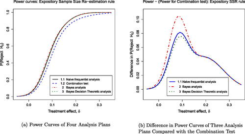
Table 2 Properties of four plans under the expository sample size re-estimation rule.

Statistical analysis plan	$P_{\delta }(\text{Reject}{H}_0)$			E(Loss)
	δ = 0	$\delta =0.1$	$\delta =0.2$
1.1 Naive frequentist test	0.033	0.587	0.952	–12.21
1.2 Combination test	0.025	0.506	0.905	–11.66
2 Bayes posterior rule	0.037	0.606	0.951	–12.17
3 Bayes decision theory	0.032	0.582	0.951	–12.22

NOTE: Results are based on 10⁷ replications, standard errors for probabilities ∼ 0.0001, standard errors for differences in E(Loss) between two plans ∼ 0.005.

In addition to presenting the probabilities of rejecting H₀ conditional on the stated value of δ, Table 2 provides the expected loss, which is an integral over both the prior distribution of δ and the trial outcomes given δ. Note that a negative loss is desirable, so the Bayes Decision Theory rule is optimal in terms of expected loss. These results show that three of the four plans have an inflated Type I error rate, while the combination test is effective in maintaining the original Type I error rate of 0.025. This is despite the fact that early stopping to reject H₀ takes place when ${\widehat{\delta }}_1>0.3$ and this was not assumed to be the case when defining the combination test. The reason this early stopping to reject H₀ has so little impact is that such a high value of ${\widehat{\delta }}_1$ is highly unlikely when δ = 0 (with probability less than ${10}^{-4}$). Even if such a value does occur, it is quite likely that H₀ would be rejected were the trial to continue with a positive post-disruption sample size.

It is to be expected that the naive frequentist test has an inflated Type I error rate: when the initial results are unpromising, a high post-disruption sample size gives almost a fresh opportunity to see a false positive result, but when initial results are more favorable for the new treatment, a small post-disruption sample size helps preserve this pattern. The fact that the Type I error rate for the two Bayesian analyses have similarly inflated probabilities of rejecting H₀ under δ = 0 may be more surprising since the calculation of the posterior distribution is not affected by how N₂ might have been chosen had other values of ${\widehat{\delta }}_1$ been observed. However, the posterior distribution in a Bayesian analysis conditions on observed data rather than on a particular value of the parameter δ. The results show that the probability of a false positive result can increase by essentially the same mechanism as for the naive frequentist test when initially promising results are retained by decreasing the post-disruption sample size while unpromising results are diluted by a much higher post-disruption sample size.

One might, however, question the need to preserve Type I error rate from a Bayesian perspective. In particular, if the elements of the Bayes decision problem are viewed as appropriate to the problem, it is natural to retain these elements (the values of B and L in our case). By definition, Plan 3 minimizes the expected loss and this is evident from the results in Table 2. Interestingly, it is only the combination test that has a markedly higher expected loss and this appears to be a consequence of that plan’s stricter control of the Type I error rate.

The Realistic Sample Size Rule

Turning now to the “Realistic” SSR rule, Figure 6 shows power curves for the four plans and Table 3 presents properties of these procedures. The changes in sample size are more modest in this case, with the post-disruption sample size N₂ varying between 100 and 300 patients per treatment arm. The impact is reduced accordingly, although the pattern of results remains the same. The combination test provides strict protection of the Type I error rate while the other three plans show a small inflation in this error rate and higher power under $\delta =0.1$ and $\delta =0.2$. The Bayes decision theory analysis minimizes expected loss for the specified loss function, although Plans 1.1 and 2 also achieve the same expected loss to two decimal places.

Fig. 6 Power curves for the realistic sample size re-estimation rule: (a) shows the power curves for the four different plans. (b) shows the slightly higher power for each plan (1.1, 2, 3) compared to the power for the combination test: Naive (solid blue line), Bayes posterior analysis (dashed red line), and Bayes decision theoretic (dotted green line).

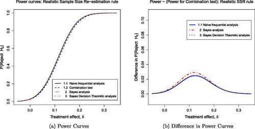
Table 3 Properties of four plans under the realistic sample size re-estimation rule.

Statistical analysis plan	$P_{\delta }(\text{Reject}{H}_0)$			$E(\mathit{\text{Loss}}$)
	δ = 0	$\delta =0.1$	$\delta =0.2$
1.1 Naive frequentist test	0.028	0.406	0.921	–10.56
1.2 Combination test	0.025	0.382	0.908	–10.50
2 Bayes posterior rule	0.029	0.410	0.922	–10.56
3 Bayes decision theory rule	0.028	0.406	0.921	–10.56

NOTE: Results are based on 10⁷ replications, standard errors for probabilities ∼ 0.0001, standard errors for differences in E(Loss) between two plans ∼ 0.005.

6 Changes to the Underlying Population

Our example trial contained inclusion and exclusion criteria that defined a target population. A disruption such as the COVID-19 pandemic may result in changes to the distribution of patient characteristics. In addition, compliance to the treatment protocol may be altered. These changes may be different for treatment and control groups. For example, lockdowns may reduce compliance with the prescribed treatment, reducing the treatment effect. We consider the scenario where there is a change in the patient population with the onset of the disruption and how this might impact the analysis. This change could be represented by a known factor, such as time of recruitment into the study or a patient’s observed COVID-19 status, or represented as an unknown factor that captures the population differences but is not observed at the individual patient level.

6.1 When Population Status is Known

As an example, assume the populations after the onset of the disruption are defined by their known observed COVID-19 status. Then we can simply include a COVID-19 indicator covariate in the linear model and add a parameter β_c in the regression model. The model might allow for an interaction between COVID-19 status and the treatment effect, as in (10) $$Y_i|C_i,T_i,\Theta \sim N\left({\mu }_0+\delta T_i+{\beta }_c{C}_i+{\gamma }_c{C}_i{T}_i,{\sigma }^2\right)$$(10) where $i=1,\dots ,m_0+m_1$ indexes patients; m₀ and m₁ are the numbers of patients in the control and treatment group, respectively; T_i is the treatment assignment indicator (T_i=0 for the control group; T_i=1 for the new treatment group); C_i is a covariate that is an indicator of patient i having the condition associated with the disruption (e.g., COVID-19); μ₀ is the mean response for the control group without the condition, δ is the effect of the new treatment, β_c is the effect of the condition; and γ_c is the interaction effect of the condition within treatment group. The set of model parameters is $\Theta =({\mu }_0,\delta ,{\beta }_c,{\gamma }_c)$; ${\sigma }^2$ is known.

Letting μ_i be the expected value for patient i, the resulting likelihood is (11) $$\prod _{i=1}^{m_0+m_1}\frac{1}{\sigma }\varphi \left[\frac{{(y_i-{\mu }_i)}^2}{{\sigma }^2}\right],$$(11) where $\varphi$ denotes the probability density of a N(0, 1) random variable. We note that in this section we assume that the parameters of interest (e.g., δ) among all model parameters (Θ) in the statistical model retain the same meaning throughout the course of the trial. This assumption may not be tenable and may lead to challenges in interpretation of the analyses or require changes in the prior distribution (see Section 6.2).

Bayesian Approaches

Bayesian statistical methodology is useful for assessing how changes in the patient population might affect the final analysis of the data before and after the onset of the disruption if the trial resumes. Predicting future outcomes via the predictive distribution allows one to carry out various sensitivity analyses to inform decisions regarding the resumption of the trial as originally planned or with changes. We assume that equation (10)(10) $$Y_i|C_i,T_i,\Theta \sim N\left({\mu }_0+\delta T_i+{\beta }_c{C}_i+{\gamma }_c{C}_i{T}_i,{\sigma }^2\right)$$(10) is the model for inference.

As mentioned in Appendix B.3 in the supplementary material, there are Bayesian designs that use the predictive distribution rather than the posterior distribution to inform decision-making at interim analyses. These interim analyses typically predict the final hypothesis test in a trial given current data, yielding a distribution. If one is concerned that the post-disruption population distribution may differ from the pre-disruption population, one can calculate the predictive distribution to infer what might be the outcome of the trial had the disruption not occurred. If $p^{\star }({\mathbf{Y}}_{\text{new}}|\Theta )$ denotes some hypothesized sampling distribution after the trial restarts, then one can carry out simulations with $\int p^{\star }({\mathbf{Y}}_{\text{new}}|\Theta )p(\Theta |{\mathbf{Y}}_{\text{current}})d\Theta$ and compare the results with $p({\mathbf{Y}}_{\text{new}}|{\mathbf{Y}}_{\text{current}})$, the sampling distribution in the original statistical model. Future observations are independent conditional on pre-disruption data. This independence can be used to re-design future trials conditional on the past.

Frequentist Approaches

Frequentist methods may be based on the regression equation (10)(10) $$Y_i|C_i,T_i,\Theta \sim N\left({\mu }_0+\delta T_i+{\beta }_c{C}_i+{\gamma }_c{C}_i{T}_i,{\sigma }^2\right)$$(10) and/or the likelihood equation (11)(11) $$\prod _{i=1}^{m_0+m_1}\frac{1}{\sigma }\varphi \left[\frac{{(y_i-{\mu }_i)}^2}{{\sigma }^2}\right],$$(11) to estimate parameters and test hypotheses regarding the parameters, in particular, the treatment effect δ.

Calderazzo et al. (2023) describe Bayesian and frequentist methods developed for estimating δ (assuming ${\mu }_0={\beta }_c=0$) in the presence of uncertainty about γ_c, the interaction. They combine likelihoods $$L_{\mathit{\text{in}}}=\prod _{i=1}^{m_{\mathit{\text{in}}}}\frac{1}{\sigma }\varphi \left[\frac{Y_i-\delta T_i}{\sigma }\right]$$

for m_in in-study patients and $$L_{\mathit{\text{ext}}}=\prod _{i=m_{\mathit{\text{in}}}+1}^{m_{\mathit{\text{in}}}+m_{\mathit{\text{ext}}}}\frac{1}{{\sigma }_1}\varphi \left[\frac{Y_i-(\delta +{\gamma }_c)T_i}{{\sigma }_1}\right]$$ for m_ext external patients into a single estimating procedure under prior uncertainty about γ_c, where T_i is a treatment indicator. Under ${\gamma }_c=0$, δ is estimated through the MLE from a regression model fitted on $m_{\mathit{\text{in}}}+m_{\mathit{\text{ext}}}$ observations. Under ${\gamma }_c\ne 0$, datasets cannot be pooled and the MLE of δ is effectively limited to m_in observations because δ is confounded with γ_c in the external dataset. Calderazzo et al. (2023) report methods that balance between the two extremes (${\gamma }_c=0$ and ${\gamma }_c\ne 0$) to adaptively use external information.

6.2 When Population Status is Not Known

Suppose the disruption or its cause have led to concern that the treatment effect and/or baseline characteristics might be altered and affect outcomes for patients entering the study when accrual restarts after the onset of the disruption. If there are unobserved or unmeasurable changes to a subset of the population as a result of the disruption or its cause, then one probably needs to consider changing the statistical model for the post-disruption data.

One way to accommodate such population changes would be to consider the patients who enroll into the trial after the onset of the disruption to represent a mixture of two populations. That is, we may consider that the sampling distribution for the post-disruption data is a mixture, and we do not know the subpopulation to which each patient belongs. One post-disruption subpopulation may be very similar to the pre-disruption population and the other post-disruption subgroup may reflect, say, a prognostically-altered population as a result of the cause of the disruption (e.g., COVID-19).

The sampling distribution for a patient in the control or treatment group (j = 0 or 1, respectively) after the onset of the disruption is $Y_{i,j}|\Theta \sim \omega N({\mu }_{j,1},{\sigma }^2)+(1-\omega )N({\mu }_{j,2},{\sigma }^2)$, with ${\mu }_{j,1}$ the mean treatment in the first component, ${\mu }_{j,2}$ the mean in the second component of the mixture, and mixture weight ω. In this model, $\Theta =({\mu }_{0,1},{\mu }_{0,2},{\mu }_{1,1},{\mu }_{1,2},\omega )$ is the set of parameters. We could also allow for different residual variances in the two components, although our example trial assumes the variance in the data (${\sigma }^2$) is known.

The statistical model for a single patient is $$\begin{array}{c}\Theta \sim p(\Theta )\\ Y_{i,j}|\Theta \sim \omega N({\mu }_{j,1},{\sigma }^2)+(1-\omega )N({\mu }_{j,2},{\sigma }^2)\end{array}$$ where $i=1,\dots ,m_j$ indexes the patient; j = 0, 1 indexes the treatment group; the mixture weight $\omega \in (0,1)$; and ${\mu }_{j,k}$ is the mean for population k = 1, 2. Assuming the unaffected patients after the onset of the disruption have the same mean as the pre-disruption patients, then the full likelihood for pre-disruption and post-disruption data can be expressed as (12) $$\begin{array}{c}\prod _{j=0}^1 \prod _{i=1}^{m_j} {\left\{\frac{1}{\sigma }\varphi \left[\frac{y_{\mathit{\text{ij}}}-{\mu }_{j,1}}{\sigma }\right]\right\}}^{(1-D_{\mathit{\text{ij}}})}\\ \mathrm{\hspace{1em}}\mathrm{\hspace{1em}}\times {\left\{\frac{\omega }{\sigma }\varphi \left[\frac{y_{\mathit{\text{ij}}}-{\mu }_{j,1}}{\sigma }\right]+\frac{(1-\omega )}{\sigma }\varphi \left[\frac{y_{\mathit{\text{ij}}}-{\mu }_{j,2}}{\sigma }\right]\right\}}^{D_{\mathit{\text{ij}}}},\end{array}$$(12) where D_ij = 1 if patient i in treatment group j entered the trial after the onset of the disruption and D_ij = 0 otherwise, and $\varphi (·)$ is the standard normal density function.

This model does not make any assumptions about the nature of any change to the means that is attributable to the onset of the disruption (or its cause) affecting the patients or the treatment effect. We opted for this more flexible model, since subpopulation membership is unobserved.

Bayesian Approaches

In the Bayesian setting, the statistical model will now include an augmented or new prior distribution for the expanded parameter set (relative to the original pre-disruption model). It may seem reasonable to assume that the original prior model applies to the component of the mixture for the unaffected patients, and a new model applies to the parameters in the component for the affected patients. For example, let ${\mu }_{0,1}$ be the pre-disruption mean in the control group and ${\mu }_{1,1}={\mu }_{0,1}+\delta$ be the pre-disruption mean in the group assigned the new treatment. The model could include the same prior distributions for $({\mu }_{0,1},{\mu }_{1,1},\delta )$ as in the original pre-disruption model. The expanded prior model would need to include prior distributions for the mean outcomes among the post-disruption patients and for ω, that is, $({\mu }_{0,2},{\mu }_{1,2},\omega )$. We might want the pre-disruption (unaffected) data to inform the post-disruption mean outcomes with a model such as ${\mu }_{j,2}|{\mu }_{j,1}\sim N({\mu }_{j,1},{\sigma }^2/m_0)$. This prior distribution reflects, a priori, that we expect the average outcome among post-disruption patients within a treatment group to be the same as the pre-disruption mean for that same treatment group. Thus, this prior for affected patients is centered on the original prior for unaffected patients pre-disruption but allows for more variability.

What is the interpretation of the treatment effect in such models, particularly if we do not assume that the treatment difference after the onset of the disruption is the same as for the pre-disruption patients [i.e., $({\mu }_{1,1}-{\mu }_{0,1})\ne ({\mu }_{1,2}-{\mu }_{0,2})$]. Consider our example diabetes trial and COVID-19 as the cause of the disruption. Even if we assume that the baseline HbA1c has changed for one of the populations after the onset of the disruption (e.g., those who had COVID-19), then it is still possible for the treatment effect (δ) to have the same prior specification as before and not be a mixture. We have ${\mu }_{0,1}$ denoting the 6-month difference in HbA1c for the control patients who have not had COVID-19, and ${\mu }_{1,1}$ as the 6-month change for the patients who received the new treatment but never had COVID-19. Let ${\delta }_1={\mu }_{1,1}-{\mu }_{0,1}$. After the onset of the disruption, the treatment effect may be altered for those who have had COVID-19. Set ${\delta }_2={\mu }_{1,2}-{\mu }_{0,2}$. We might consider the same prior distribution for both δs if we consider it likely that ${\delta }_1={\delta }_2=\delta$, where δ is the treatment effect in the statistical model for pre-disruption patients. That is, we might consider ${\delta }_1,{\delta }_2\sim p(\delta )$ with $p(\delta )$ the prior as specified in the original protocol. Such an assumption would seem reasonable, as long as a priori we had $p(\delta ,{\mu }_0)=p(\delta )p({\mu }_0)$, that is, independent priors.

Another possible revision to the prior distribution would be to consider a hierarchical model for key model parameters before and after the onset of the disruption. To allow for different values of δ before and after the disruption, set up two models, each with its own treatment effect. For example, we might have $f({\mathbf{Y}}_{\text{pre‐disruption}}|{\delta }_1)$ for the pre-disruption data and $f({\mathbf{Y}}_{\text{post‐disruption}}|{\delta }_2)$ for data collected after the onset of the disruption. One might propose a hierarchical prior distribution for $({\delta }_1,{\delta }_2)$, viz., ${\delta }_1,{\delta }_2|\xi \sim p(\delta |\xi )$ with a prior distribution $p(\xi )$ for the hyperparameter ξ. The prior distribution for ξ could be the distribution in the original protocol for δ, perhaps with some larger variance. This model would allow the possibility that ${\delta }_1\ne {\delta }_2$, but also provide shrinkage in the estimation of the two posterior estimates. That is, this model allows the reasonable assumption that the treatment effect, say, is similar before and after the disruption, while allowing some probability that the treatment effect changes. The amount of shrinkage would depend on the differences inherent in the data and the between-δ variance in the prior $p(\delta |\xi )$.

Another alternative Bayesian model would be something akin to the robust meta-analytic-predictive (MAP) prior (Schmidli et al. 2014). Let δ be the parameter of interest, and ${\mathbf{Y}}_{\text{current}}$ be the patient data available at the time of the disruption-related analysis. The robust MAP is $$ϵ p(\delta |{\mathbf{Y}}_{\text{current}})+(1-ϵ)p_0(\delta ).$$

In this mixture, $p(\delta |{\mathbf{Y}}_{\text{current}})$ is the posterior distribution of δ at the time of the analysis based on currently available data, $p_0(\delta )$ is the protocol-specified prior distribution, and $ϵ\in (0,1)$ is a weighting factor. One might use this mixture prior distribution to analyze data collected once the trial resumes after the onset of the disruption. The MAP prior or something like it for repeated analyses accounting for change during and after the onset of the disruption (Wang et al. 2023) may be more applicable or more easily defended to regulators when dealing with the effects of a disruption.

If a Bayesian analysis in response to the disruption considers a different prior distribution than the prior specified in the protocol, then the resulting posterior distribution may lead to decisions that exhibit different operating characteristics than those given in the protocol. Simulations prior to the actual analysis could assess possible differences from the specifications in the protocol and discuss options with the trial’s stakeholders. One would compare results using the new prior to the frequentist characteristics with the original prior to assess future risks.

Despite its relative parsimony, the mixture model might not fit the data well. The fit will depend extensively on the amount of information available for the pre-disruption population and related subgroup of the patients entering after the onset of the disruption.

An even more flexible approach would be a Bayesian nonparametric prior model to the treatment effect alone or to several clinically important parameters (Müller et al. 2015). In this way, the data will inform the posterior inference if there are heterogeneities across patients in important clinical factors that are captured by the statistical model.

Careful consideration would have to apply if one characterizes the post-disruption data as a mixture. The data might not support the inference implied by the assumption that the same treatment effect pre-disruption is experienced by one of the post-disruption subgroups. Simulations could help answer questions about how different types of disruption-related changes might affect inference, as well as provide estimates of long-term effects of the disruptions on error probabilities.

Considering constraints imposed by working within the regulatory environment, the Bayesian may have to make changes to decision rules to satisfy regulators. Such constraints mean that the Bayesian has less freedom to make certain changes without altering the design. Regulators wish to protect against the introduction of medical products that are not adequately safe and effective. As a result, regulators will be concerned that the data and analyses upon which they make approval decisions accurately reflect the study results and satisfy regulatory considerations. Furthermore, the regulators will want to feel that any treatment effect seen in the trial can reasonably be expected to apply outside of the trial. Reviewers may be hesitant to accept mid-trial changes to prior distributions without strong justification and evaluation of potential consequences of any changes. There will likely be discussions among the stakeholders about the robustness of inferences if there are changes to the prior distribution.

Frequentist Approaches

Without the specification of prior distributions, frequentist methods for estimating the parameters of the mixture distribution can be challenging, as noted by Kieser, Friede, and Gondan (2013), Titterington, Smith, and Makov (1985), and Lindsay (1995). In particular, Lindsay (1995) describes problems concerning convergence issues which may relate to problems of identifiability.

One possible approach is to consider baseline patient covariates to account for the population marker in a regression model similar to equation (10)(10) $$Y_i|C_i,T_i,\Theta \sim N\left({\mu }_0+\delta T_i+{\beta }_c{C}_i+{\gamma }_c{C}_i{T}_i,{\sigma }^2\right)$$(10) (Food and Drug Administration 2023). For example, our simple trial might include the baseline HbA1c and look at the patient’s HbA1c at 6 months (which, as noted in Section 2.1, is a more efficient design than using the difference in the mean change at 6 months). This covariate analysis could be expanded to evaluate time-dependent population changes as the disruption continues (Van Lancker et al. 2022, sect. 2.2). However, the model fit would need to be assessed as well as the possibility of an interaction between the cause of the disruption and treatment effect.

7 Discussion and Conclusions

A disruption to an ongoing clinical trial, such as caused by the COVID-19 pandemic, raises many questions for clinical trialists and clinical trial statisticians in particular.

We have compared different approaches to analyzing a clinical trial when the design is modified after a disruption. We defined a frequentist hypothesis test and two Bayesian analyses, one based directly on the posterior distribution of the treatment effect δ, the other with a decision theory formulation. We specified the Type I error rate, prior distribution, and loss function in these analyses so that all three would give the same conclusion if the trial ran according to the original plan with no disruption. We then applied these methods when the trial’s final sample size was modified following a disruption after 60% of the planned number of patients had been recruited and their responses recorded.

In the simplest response to a disruption (Section 3.1), the study team decides to make design changes that do not depend on pre-disruption data. Pre- and post-disruption data remain independent and the revised model may contain some new covariates, but planning for the final analysis at the time of the disruption is essentially the same as if the modifications had been planned before the trial has commenced.

In Sections 3.2.1 and 3.2.2, we describe how the probabilities of modification under various scenarios can be calculated and used to obtain the joint distribution of the pre-disruption data and the post-disruption data (if the study continued) and a most powerful end-of-study test $H_0:\delta =0$ at the desired Type I error rate. The popular combination test is used to approximate the sampling distribution of the final summary test statistic (Section 3.2.3). This approximation does not need to specify the decision probabilities at the time of disruption; the pre- and post-disruption data can be combined with fixed weights as independent data. With the combination test, Type I error rates can be preserved exactly regardless of the way in which the trial design was modified. Section 3.3 shows how it can be applied when the trial design is modified after the pre-disruption response data have been observed.

In Section 5.4 we use simulations to evaluate the impact on the Type I error when selecting a post-disruption sample size based on the observed pre-disruption treatment effect $\widehat{\delta }$. We compared four analysis plans: two frequentist plans—a “Naive” plan (Section 3.2.1) and the combination test (Section 3.2.1); and two Bayesian approaches—one based on the posterior distribution of δ (Section 2.3.1) and a Bayesian decision theoretic plan based on minimizing expected loss (Section 2.3.2). The simulated trials found that for the two Bayesian analyses, the increase in Type I error rate above the target value $\alpha =0.025$ was similar to that seen for a Naive frequentist analysis which applied a level α significance test to the final set of data, ignoring the data-dependent sample size modifications.

If the trial design is modified based on knowledge of the pre-disruption data, it can be difficult to define a Type I error rate. The specific sample size re-calculation rules followed in Sections 3.2.1 and 5 are arbitrary examples. The combination test has the useful feature of guaranteeing the Type I error rate regardless of how the sample size might have been recalculated. However, in a Bayesian analysis, inferences are based on the posterior distribution of the treatment effect δ given the observed data and this distribution is not affected by what might have been done in situations that did not actually occur. One might argue that, since the Bayesian decision rules were acceptable for the original study design, they should also be acceptable to apply these in a modified design. For instance, if the loss function in a Bayesian decision theory rule provides the correct balance between the benefits of identifying an effective treatment and the risk of approving an ineffective treatment, then it should also do so when data come from a modified trial design. In our examples, the values of expected loss for different methods show the Bayes decision rule is clearly superior to the combination test for this criterion.

In Section 4, we illustrated how Bayesian approaches to sequential designs could handle disruptions to the Bayesian designs described in Section 2.3. Bayesian methods (Section 4) are useful for making early decisions. For example, stopping to reject the null hypothesis if the posterior distribution for δ is predominantly above zero or there is a large difference in posterior expected loss for the decisions “Reject H₀” and “Accept H₀”. Although there could be consequences for the Type I error rate, stopping for futility would, in general, only decreases the Type I error.

In Section 6 we discussed how the treatment effect or the distribution of patient characteristics and treatment compliance could change after the onset of a disruption. Some characteristics, for example, being infected by COVID-19, may not be known for all patients. Where possible, one may model patient response in terms of observed factors (Section 6.1). When a post-disruption condition cannot be described by an observable factor at the individual patient level, responses for patients enrolled after the onset of the disruption could be modeled as a mixture of two populations (Section 6.2). Fitting complex models to partially observed data is challenging, but Bayesian inference, with the posterior parameter distribution obtained by Markov chain Monte Carlo simulation, can overcome the computational problems as long as an appropriate model has been formulated.

We take three key points from our investigations. The first, perhaps primarily from a frequentist perspective, is that if a disruption occurs and the study team have not yet seen any patient response data, they should remain blinded to such data while they define rules for implementing design modifications. It will then be possible to respond to the pre-disruption data in a way that controls the Type I error rate unambiguously. The rules that are defined may be sophisticated, for example, group sequential stopping could be introduced, including the option of stopping at the onset of disruption, or a sample size re-calculation rule may be specified so that the modified sample size will depend on the interim data in a pre-determined way. Second, for both frequentist and Bayesian designs, we note it is beneficial to have a sequential stopping rule included in the original trial design: as well as the usual benefits for trial efficiency, a suitably defined rule could facilitate stopping at the onset of disruption based on the evidence in data observed thus far. Third, the COVID-19 pandemic highlights the potential for disruptions to alter patient characteristics, treatment compliance, and supportive or ancillary care, any of which could affect outcome. Initial study designs should include baseline patient covariates that could be useful for monitoring and perhaps accounting for changes in the pre-disruption versus post-disruption population and even changes in the treatment effect.

In our consideration of frequentist and Bayesian approaches to mitigating the effects of unplanned clinical trial disruptions, we have identified a number of open research questions:

1. If the trial resumes after the onset of the disruption, what statistical model would be most appropriate?

2. When is it necessary to account for pre-disruption patients separately from patients enrolled after the onset of the disruption?

3. If a disruption leads to an analysis that changes the sample space, how might one incorporate such changes in the statistical model?

4. There is a substantial literature on interim decision rules used on sequential tests and sample size re-estimation procedures. Can this work be extended to inform the choice of design modifications following a disruption?

5. How should the prior distribution be adjusted if new prognostic factors become known among some trial patients who were differentially affected by the cause of the disruption?

6. Bayesian and other adaptive trial designs offer great flexibility for adaptation, but regulators typically want decision rules and potential adaptations to be specified in the protocol before the trial commences [Food and Drug Administration (2019)]:

   • If the investigators designed the trial with a Bayesian analysis in a manner that satisfies regulators, how can they make changes in response to the disruption or any lasting effects of the factors that led to the disruption.

   • Could one incorporate new previously unavailable information into the analysis, particularly with respect to augmenting the prior distribution or statistical model in light of external information?

7. Knowing what we know now, more than three years after the onset of the COVID-19 pandemic caused major worldwide disruption and affected the health status of millions of people, how might we design future trials to make them more robust to the impact of another pandemic-related disruption?

8. When should we consider designing clinical trials based on the assumption that data will be analyzed with strata or covariates based on blocks of calendar time to allow for external factors that might affect the patients or treatment while the trial is ongoing?

We look forward to seeing the results of further research on these topics.

Supplementary Materials

Below is a list of the file names and brief descriptions of R code that can be found in the supplementary material. The R code files are included in zip file “R code for Bayesian and Frequentist Approaches to Rescuing Disrupted Trials Kunz et al.zip.”

LRT_with_SSR.R:(Section 3.2.1) R code for designing the most powerful test of a simple null versus a simple alternative hypothesis with a pre-determined interim sample size recalculation rule. The two sample size recalculation rules used by this R code are defined in Table 1 of Section 3.2.1. This file includes R code for Figure 2.

GenerateDiabetesData.R:(Section 2.3) Simulate diabetes data with baseline and 6-month HbA1c.

CalibratedPriorBayesianDesign.R:(Section 2.3.1) Program to compute prior sample size for calibrated Bayesian prior distribution and simulate the design to determine the frequentist operating characteristics of the design when the true delta is 0 and when it equals 0.2.

BayesianDecisionTheoreticDesign_ForPaper.R:(Section 2.3.2) Prog- ram to evaluate a decision-theoretic design. The design and utility function are based on Berry and Ho (1988).

PlotsForPaper.RR code for figures 1, 3, and 4:

Figures 1a, b(Section 2.3) The prior and posterior distributions, for the likelihood under $\widehat{\delta }=0$ and $\widehat{\delta }=0.2$.

Figures 3a, b(Section 4.1) Prior and posterior distributions for the skeptic and enthusiast under two different scenarios.

Figure 4(Section 4.1) Skeptic’s and enthusiast’s predictive distributions for the final test statistic if the trial were to continue to enroll all 1000 patients, given the interim data at the onset of disruption.

Figures-5-and-6.R(Section 5.4) Program to generate Figures 5 and 6, which show power curves for four hypothesis testing procedures.

Acknowledgments

The authors thank the National Institute of Statistical Sciences and its Director, James L. Rosenberger, for facilitating Session 6 of the Ingram Olkin forum series on “Bayesian and frequentist approaches to rescuing disrupted trials.” The authors would also like to recognize the organizers of the Ingram Olkin Forum Series on Unplanned Clinical Trial Disruptions: Nancy Flournoy (chair), Jonathan Bartlett, Chris Jennison, Adam Lane and Sergey Tarima.

Disclosure Statement

The authors report that there are no conflicts of interests to declare.

Additional information

Funding

R.E. is funded by UK National Institute for Health and Care Research (NIHR300051) and NIHR Maudsley Biomedical Research Centre (NIHR203318). N.S. is partially supported by the UK Medical Research Council (grant numbers MR/V038419/1 and MR/W021013/1). S.Z. is partially supported by the PEPR SN SMATCH France 2030 ANR-22-PESN-0003.

References

- Bauer, P., and Kohne, K. (1994), “Evaluation of Experiments with Adaptive Interim Analyses,” Biometrics, 50, 1029–1041.
- Bellman, R. (1957), Dynamic Programming, Princeton, NJ: Princeton University Press.
- Berry, D., and Ho, C. (1988), “One-Sided Sequential Stopping Boundaries for Clinical Trials: A Decision-Theoretic Approach,” Biometrics, 44, 219–227.
- Brockwell, A. E., and Kadane, J. B. (2003), “A Gridding Method for Bayesian Sequential Decision Problems,” Journal of Computational and Graphical Statistics, 12, 566–584. DOI: 10.1198/1061860032274.
- Calderazzo, S., Tarima, S., Reid, C., Flournoy, N., Friede, T., Geller, N., Rosenberger, J. L., Stallard, N., Ursino, M., Vandemeulebroecke, M., Van Lancker, K., and Zohar, S. (2023), “Coping with Information Loss and the Use of Auxiliary Sources of Data: A Report from the NISS Ingram Olkin Forum Series on Unplanned Clinical Trial Disruptions,” Statistics in Biopharmaceutical Research, 1–17. Advanced online publication. DOI: 10.1080/19466315.2023.2211023.
- Carlin, B. P., Kadane, J. B., and Gelfand, A. E. (1998), “Approaches for Optimal Sequential Decision Analysis in Clinical Trials,” Biometrics, 54, 964–975.
- Colantuoni, E., and Rosenblum, M. (2015), “Leveraging Prognostic Baseline Variables to Gain Precision in Randomized Trials,” Statistics in Medicine, 34, 2602–2617. DOI: 10.1002/sim.6507.
- Committee for Medicinal Products for Human Use. (2007), Reflection Paper on Methodological Issues in Confirmatory Clinical Trials Planned with an Adaptive Design, London, UK: European Medicines Agency.
- Cui, L., Hung, H. J., and Wang, S.-J. (1999), “Modification of Sample Size in Group Sequential Clinical Trials,” Biometrics, 55, 853–857. DOI: 10.1111/j.0006-341x.1999.00853.x.
- DeGroot, M. H. (2004). Optimal Statistical Decisions. Hoboken, N.J.: John Wiley & Sons, Inc.
- Dmitrienko, A., D’Agostino Sr., R. B., and Huque, M. F. (2013), “Key Multiplicity Issues in Clinical Drug Development,” Statistics in Medicine, 32, 1079–1111. DOI: 10.1002/sim.5642.
- Evans, S. (2007), “When and How Can Endpoints be Changed After Initiation of a Randomized Clinical Trial,” PLoS Clinical Trials, 2, e18. DOI: 10.1371/journal.pctr.0020018.
- Flournoy, N., and Tarima, S. (2023), “Discussion on “Adaptive Enrichment Designs with a Continuous Biomarker” by Nigel Stallard,” Biometrics, 79, 31–35. DOI: 10.1111/biom.13641.
- Food and Drug Administration. (2019), Adaptive Designs for Clinical Trials of Drugs and Biologics - Guidance for Industry, Silver Spring, MD: U.S. Department of Health and Human Services.
- ——— (2023), Adjusting for Covariates in Randomized Clinical Trials for Drugs and Biological Products Guidance for Industry, Silver Spring, MD: U.S. Department of Health and Human Services, Food and Drug Administration, Center for Drug Evaluation and Research (CDER) and Center for Biologics Evaluation and Research (CBER) and Oncology Center for Excellence (OCE).
- Freedman, L. S., and Spiegelhalter, D. J. (1992), “Application of Bayesian Statistics to Decision Making During a Clinical Trial,” Statistics in Medicine, 11, 23–35. DOI: 10.1002/sim.4780110105.
- Friede, T., and Kieser, M. (2003), “Blinded Sample Size Reassessment in Non-inferiority and Equivalence Trials,” Statistics in Medicine, 22, 995–1007. DOI: 10.1002/sim.1456.
- Graf, A. C., and Bauer, P. (2011), “Maximum Inflation of the Type I Error Rate When Sample Size and Allocation Rate are Adapted in a Pre-planned Interim Look,” Statistics in Medicine, 30, 1637–1647. DOI: 10.1002/sim.4230.
- Jennison, C., and Turnbull, B. (1999), Group Sequential Methods with Applications to Clinical Trials, Chapman & Hall/CRC Interdisciplinary Statistics, Boca Raton, FL: CRC Press.
- Jennison, C., and Turnbull, B. W. (2013), “Interim Monitoring of Clinical Trials: Decision Theory, Dynamic Programming and Optimal Stopping,” Kuwait Journal of Science, 40, 43–50.
- Khunti, K., Godec, T. R., Medina, J., Garcia-Alvarez, L., Hiller, J., Gomes, M. B., Cid-Ruzafa, J., Charbonnel, B., Fenici, P., Hammar, N., Hashigami, K., Kosiborod, M., Nicolucci, A., Shestakova, M. V., Ji, L., and Pocock, S. (2018), “Patterns of Glycaemic Control in Patients with Type 2 Diabetes Mellitus Initiating Second-Line Therapy after Metformin Monotherapy: Retrospective Data for 10,256 Individuals from the United Kingdom and Germany,” Diabetes, Obesity and Metabolism, 20, 389–399. DOI: 10.1111/dom.13083.
- Kieser, M., and Friede, T. (2003), “Simple Procedures for Blinded Sample Size Adjustment That Do Not Affect the Type I Error Rate,” Statistics in Medicine, 22, 3571–3581. DOI: 10.1002/sim.1585.
- Kieser, M., Friede, T., and Gondan, M. (2013), “Assessment of Statistical Significance and Clinical Relevance,” Statistics in Medicine, 32, 1707–1719. DOI: 10.1002/sim.5634.
- Lindsay, B. G. (1995), Mixture Models: Theory, Geometry, and Applications, Hayward, CA: Institute of Mathematical Statistics.
- Little, R. J. (2006), “Calibrated Bayes: A Bayes/Frequentist Roadmap,” The American Statistician, 60, 213–223. DOI: 10.1198/000313006X117837.
- Müller, H.-H., and Schäfer, H. (2004), “A General Statistical Principle for Changing a Design Any Time During the Course of a Trial,” Statistics in Medicine, 23, 2497–2508. DOI: 10.1002/sim.1852.
- Müller, P., Quintana, F., Jara, A., and Hanson, T. (2015), Bayesian Nonparametric Data Analysis, Springer Series in Statistics, Cham: Springer.
- O’Brien, P. C., and Fleming, T. R. (1979), “A Multiple Testing Procedure for Clinical Trials,” Biometrics, 35, 549–556.
- Orkin, A. M., Gill, P. J., Ghersi, D., Campbell, L., Sugarman, J., Emsley, R., Steg, P. G., Weijer, C., Simes, J., Rombey, T., Williams, H. C., Wittes, J., Moher, D., Richards, D. P., Kasamon, Y., Getz, K., Hopewell, S., Dickersin, K., Wu, T., Ayala, A. P., Schulz, K. F., Calleja, S., Boutron, I., Ross, J. S., Golub, R. M., Khan, K. M., Mulrow, C., Siegfried, N., Heber, J., Lee, N., Kearney, P. R., Wanyenze, R. K., Hróbjartsson, A., Williams, R., Bhandari, N., Jüni, P., Chan, A.-W., and C. Group, (2021), “Guidelines for Reporting Trial Protocols and Completed Trials Modified Due to the COVID-19 Pandemic and Other Extenuating Circumstances: The CONSERVE 2021 Statement,” JAMA, 326, 257–265. DOI: 10.1001/jama.2021.9941.
- Pocock, S. J. (1977), “Group Sequential Methods in the Design and Analysis of Clinical Trials,” Biometrika, 64, 191–199. DOI: 10.1093/biomet/64.2.191.
- Proschan, M. A., Follmann, D. A., and Waclawiw, M. A. (1992), “Effects of Assumption Violations on Type I Error Rate in Group Sequential Monitoring,” Biometrics, 48, 1131–1143. DOI: 10.2307/2532704.
- Proschan, M. A., and Hunsberger, S. A. (1995), “Designed Extension of Studies based on Conditional Power,” Biometrics, 51, 1315–1324.
- Schmidli, H., Gsteiger, S., Roychoudhury, S., O’Hagan, A., Spiegelhalter, D., and Neuenschwander, B. (2014), “Robust Meta-Analytic-Predictive Priors in Clinical Trials with Historical Control Information,” Biometrics, 70, 1023–1032. DOI: 10.1111/biom.12242.
- Spiegelhalter, D. J., Freedman, L. S., and Parmar, M. K. B. (1994), “Bayesian Approaches to Randomized Trials,” Journal of the Royal Statistical Society, Series A, 157, 357–387. DOI: 10.2307/2983527.
- Stallard, N. (2023), “Adaptive Enrichment Designs with a Continuous Biomarker,” Biometrics, 79, 9–19. DOI: 10.1111/biom.13644.
- Tarima, S., and Flournoy, N. (2019), “Distribution Theory Following Blinded and Unblinded Sample Size Re-estimation under Parametric Models,” Communications in Statistics-Simulation and Computation, 51, 1–12.
- Tarima, S., and Flournoy, N. (2022), “Most Powerful Test Squences with Early Stopping Options,” Metrika, 85, 491–513. DOI: 10.1007/s00184-021-00839-w.
- Titterington, D., Smith, A., and Makov, U. (1985), Statistical Analysis of Finite Mixture Distributions, New York: Wiley.
- Van Lancker, K., Tarima, S., Bartlett, J., Bauer, M., Bharani-Dharan, B., Bretz, F., Flournoy, N., Michiels, H., Parra, C. O., Rosenberger, J. L., and Cro, S. (2022), “Estimands and their Estimators for Clinical Trials Impacted by the COVID-19 Pandemic: A Report from the NISS Ingram Olkin Forum Series on Unplanned Clinical Trial Disruptions,” Statistics in Biopharmaceutical Research, 15, 94–111. DOI: 10.1080/19466315.2022.2094459.
- Vickers, A. J. (2001), “The Use of Percentage Change from Baseline as an Outcome in a Controlled Trial is Statistically Inefficient: A Simulation Study,” BMC Medical Research Methodology, 1, 6. DOI: 10.1186/1471-2288-1-6.
- Wang, C., Lin, M., Rosner, G. L., and Soon, G. (2023), “A Bayesian Model with Application for Adaptive Platform Trials Having Temporal Changes,” Biometrics, 79, 1446–1458. DOI: 10.1111/biom.13680.
- Wittes, J., and Brittain, E. (1990), “The Role of Internal Pilot Studies in Increasing the Efficiency of Clinical Trials,” Statistics in Medicine, 9, 65–72. DOI: 10.1002/sim.4780090113.