Work conjugate pair of stress and strain in molecular dynamics

ABSTRACT

Certain stress and strain form a thermodynamic conjugate pair such that their strain energy equals to a scalar-valued potential energy. Different atomistic stresses and strains are analytically derived based on the work conjugate relation. It is numerically verified with both two-body and three-body potentials that the atomistic Kirchhoff stress, first-order Piola–Kirchhoff stress and second-order Piola–Kirchhoff stress are conjugates to atomistic logarithmic strain, deformation gradient and Lagrangian strain, respectively. Virial stress at 0 K based on original volume is the special form of atomistic Kirchhoff stress for pair potential. It is numerically verified that Hencky strain is not conjugate to any stress.

KEYWORDS:

• Thermodynamic conjugacy
• logarithmic strain
• atomistic stress
• deformation gradient
• strain energy
• interatomic potential
• Tersoff potential
• atomistic first-order Piola–Kirchhoff stress
• atomistic second-order Piola–Kirchhoff stress
• atomistic Kirchhoff stress
• virial stress

1. Introduction

Stress tensor and strain tensor are fundamental in continuum mechanics (CM). In finite strain theory, stress and strain can take different forms that can often be converted to each other. Certain stress tensor and strain tensor form a conjugate pair such that the stress integrates over the strain yields a scalar-valued potential energy [1]. Only the conjugate pair of stress and strain should be chosen as dependent and independent constitutive variables, respectively, otherwise the existence of a scalar-valued potential energy is not guaranteed. The following conjugate pairs, (1) second-order Piola–Kirchhoff stress (PK2) and Lagrangian strain, (2) Hencky strain and Kirchhoff stress [2–4], (3) first-order Piola–Kirchhoff stress (PK1) and deformation gradient, have been mentioned. It is worthwhile to note that Cauchy stress tensor is not conjugate to any strain tensor, therefore it may not be directly used in constitutive equation.

As an effort to bridge the gap between molecular dynamics (MD) and CM, it is vitally important to define stress and strain at atomistic level. Large-strain tensorial definitions of stress and strain at atomistic level allow the results of MD be expressed in the form of stress–strain relation, which can be directly fed into the material model of CM [5]. This sequential multi-scale approach may potentially replace material testing in the development of material model for finite element analysis [6,7].

The concepts of stress and strain are well understood in CM. The atomistic definitions of stress and strain, on the contrary, are still in the developmental stage [8–11]. Notice that the definitions of the stress and strain in CM require the material points to be infinitesimally small, which is certainly not true in MD due to its discrete description and the finiteness of the atomistic mass. To formulate stress tensor in CM, the concept of the mass of a material point needs to be replaced by that of mass density. The force equilibrium leads to the conclusion that stress follows tensorial transformation rule. Now let us formulate the stress tensor not based on the concept of infinitesimal mass point. The balance of moment is applied (cf. Equation (1)) over the material of a finite size tetrahedron (cf. Figure 1)

(1)

Figure 1. Tetrahedron [1].

where is the mass density at some interior point in volume , is the acceleration vector at some interior point of , is the body force, and are the surface traction per unit area at some point on surface area and , respectively. Divide both side by

(2)

where is unit normal.

Assumption 1

In the limiting case, the ratio of volume over surface area is vanishingly small, i.e. . Therefore, the inertia effect and body force effect (last two terms of Equation (2)) can be neglected. This generally means the size of the system has to be relatively small.

Assumption 2

In the static equilibrium case with no body force and acceleration, the last two terms of Equation (2) vanishes.

Accepting either Assumption 1 or Assumption 2 leads to

(3)

The stress tensor is the -th component of the stress vector acting on the positive side of the -th coordinate surface. In other words,

(4)

where is the unit vector along -axis. Because both and are tensorial quantities, so is stress tensor [1]. Without such assumption, there is no rigorous definition for atomistic stress.

In the derivation of strain in CM, the displacement field has to be continuous and smooth to enable the calculation of deformation gradient. In MD simulation, the displacement field is discrete; without further assumption, the rigorous definition of strain does not exist. We thus assume that all atoms follow a single uniform deformation gradient [12]. Under such assumption, all forms of strains, such as Lagrangian strain and Eulerian strain, can be rigorously defined and calculated.

Many researchers have defined various atomistic stresses [10,13–17]. The most commonly used atomistic stress is virial stress of statistical mechanics. The derivation process offers no clue to tell which is the equivalence of virial stress in CM. Without knowing its equivalence, it is impossible to choose its conjugate strain in the constitutive relation.

Remark: We recall that in thermoelasticity, a branch of CM, the stress–strain–temperature relation can be expressed as

where are Cauchy stress tensor, strain tensor and temperature variation, respectively. On the other hand, the atomistic stress in MD has two parts: the potential part and the kinetic part, which are corresponding to the two parts in the above-mentioned Cauchy stress. In this work, only the potential part is considered, i.e. it is a static case of absolute zero temperature. The detailed expression of atomistic stress will be presented and discussed later.

In this article, the atomistic stress is derived based on the work conjugate relation and atomistic strain. We assume there is a single uniform deformation gradient for all atoms, therefore the strain can be defined unambiguously. The work conjugate relation requires that such stress and strain, upon integration, give total potential energy of the system, which can be readily obtained through interatomic potential. The continuum counterpart of atomistic stress and strain is identified. The conjugacy of atomistic stress and strain is numerically verified with both two-body potential and three-body potential.

2. Atomistic strain

The calculation of atomistic strain is based on the deformation gradient followed by a group of atoms. Practically, a single deformation gradient may be calculated for a group of atoms by minimizing the mapping error between the deformed and the undeformed configurations [12]

(5)

where and are the original and deformed positions of atom . Notice that a single does not always satisfy for a group of atoms [18]. Therefore, finding the single becomes a problem of optimization.

Remark: It is noticed that the Cauchy–Born rule is commonly used as a hypothesis to relate the motion of atoms in a crystal to the overall deformation of the continuum. However, for complex crystals, such as diamond or mono-layered crystalline (graphene, ), the rule needs to be modified to allow for internal degrees of freedom between the sublattices [19–22]. In this work, we follow the original idea of Cauchy–Born rule, i.e. the motion of all atoms (same kind of atoms) follow a single and uniform deformation gradient.

The Lagrangian strain can be obtained as

(6)

where is the identity matrix.

The atomistic logarithmic strain can be calculated as follows [18]. Decompose the deformation gradient as

(7)

where

(8)

are the three eigenvalues of the deformation gradient; are the three corresponding eigenvectors. Notice that is a diagonal matrix, one may define

(9)

where is the natural logarithm of . Define asymmetric logarithmic strain as

(10)

For abbreviation, the operation described by Equations (7)–(10) are named as ‘’.

(11)

The logarithmic strain is defined as the symmetric part of

(12)

Therefore Equation (12) can also be expressed as [18]

(13)

All eigenvalues of deformation gradient need to be positive in the calculation of logarithmic strain. Noticed that the natural logarithm of a negative real number is not defined (cf. Equation (9)). The atomistic logarithmic strain is objective and symmetric and is conjugate to virial stress in the case of two body potential [18] (cf. Appendix 1). Notice that the atomistic logarithmic strain is not equal to the Hencky strain. In Hencky strain calculation, one may perform polar decomposition for the deformation gradient

(14)

where is the rotational matrix. Then the Hencky strain is defined as

(15)

The logarithm is performed on the deformation gradient without the rigid body rotation [2,4]. Hencky strain is not conjugate to virial stress [18].

3. Atomistic stress

In CM, certain stress tensor and strain tensor form conjugate pair such that the strain energy, calculated by the integration of the stress over the strain, equals to the potential energy density [1]. For instance, first-order Piola–Kirchhoff stress and deformation gradient form a conjugate pair

(16)

Second-order Piola–Kirchhoff stress and Lagrangian strain form a conjugate pair;

(17)

Kirchhoff stress and logarithmic strain forms a conjugate pair [18]

(18)

where is the volume of the system in its undeformed state, is the strain energy of the system. In MD, system potential energy is explicitly given as the interatomic potential. Since a single deformation gradient can be calculated for a group of atoms, the stress can be determined by its corresponding strain through the work conjugate relation. In MD,

(19)

where is the interatomic potential energy, is the interatomic force acting on atom due to the interaction with all other atoms in the system. Consider a system of atoms, which has total potential energy

(20)

where is the total force acting on ; is the current position of . Assume the motion of all atoms follows a single uniform deformation gradient from its original position to their deformed position , , it leads to

(21)

(22)

(23)

Recall Equation (16) as

(24)

Equate Equations (23) and (24)

(25)

which implies

(26)

The atomistic first-order Piola–Kirchhoff stress is thus defined as

(27)

In this work, we adopt the first-order Piola–Kirchhoff stress tensor defined by Truesdell [23–25],

(28)

which is different from the definition given by Erigen [1,26,27]

(29)

where is the Jacobian, is the Cauchy stress tensor. Notice that

(30)

Recall the relation between first-order Piola–Kirchhoff stress and second-order Piola–Kirchhoff stress

(31)

Thus the atomistic second-order Piola–Kirchhoff stress is obtained as

(32)

The second-order Piola–Kirchhoff stress is symmetric, therefore Equation (32) can also be written as

(33)

In CM, the relation between Kirchhoff stress and the first-order Piola–Kirchhoff stress is

(34)

Recall Equation (26)

(35)

Therefore the atomistic Kirchhoff stress is defined as

(36)

which implies

(37)

Due to the symmetric nature of Kirchhoff stress, Equation (37) can be also written as

(38)

The Cauchy Stress and Kirchhoff stress are related as

(39)

Therefore the atomistic Cauchy stress becomes

(40)

where is the volume of the system in its deformed state. Because Cauchy stress is symmetric, one may write

(41)

Notice that there is no assumption that the interatomic potential is a pair potential in the derivation of Equations (27), (32) and (36). In fact, it is numerically verified that, with two body potential (Coulomb–Buckingham and Lennard–Jones) and three body potential (Tersoff), the atomistic first-order Piola–Kirchhoff stress (cf. Equation (27)) is conjugate to deformation gradient; atomistic second-order Piola–Kirchhoff stress (cf. Equation (32)) is conjugate to Lagrangian strain (cf. Equation (6)); atomistic Kirchhoff stress (cf. Equation (36)) is conjugate to atomistic logarithmic strain (cf. Equation (12)). The calculated strain energy is identically equal to the interatomic potential. It is also numerically tested that the Hencky strain as defined in Equation (15) is not conjugate to any atomistic stress.

4. Special case: atomistic stress for pair potential

Recall the system potential energy (cf. Equation (20))

(42)

Notice that is the summation of all forces acting on considering all influence within the system. It is not necessary that can be written as the summation of all contributing pair-wise forces as shown in Equation (43). For instance, the forces in Tersoff potential contain the influence of the third atom [28–30].

In the special case of two-body potential, the interatomic force on can be written as

(43)

where is the interatomic force acting on due to the interaction with . In case of pair potential, the atomistic first-order Piola–Kirchhoff stress becomes (cf. Equation (27))

(44)

Because and can be any atom within the group, Equation (44) remains valid if is interchanged with

(45)

In three-body potential

(46)

It is numerically verified that Equation (47) is not valid in three-body Tersoff potential (cf. Appendix 2) .

In two-body potential, however

(47)

therefore

(48)

Add Equations (44) and (48)

(49)

(50)

which gives , the second form of atomistic first-order Piola–Kirchhoff stress in two-body potential. It is numerically verified that only in the case of two-body potential.

It can be further derived from Equation (49) that

(51)

In two-body potential, the atomistic force vector is always parallel to the relative position vector (cf. Appendix 3).

(52)

Therefore,

(53)

(54)

(55)

(56)

Thus, it arrives at the third form of first-order Piola–Kirchhoff stress for two-body potential. Similarly, the atomistic second-order Piola–Kirchhoff stress also has its two-body form.

(57)

Interchange and

(58)

(59)

Add Equations (57) and (59)

(60)

which leads to the second form of atomistic second-order Piola–Kirchhoff stress for pair potential

(61)

Because force and relative position vector are always parallel to each other in pair potential,

(62)

(63)

(64)

(65)

which leads to the third form of atomistic second-order Piola–Kirchhoff stress for pair potential.

(66)

The atomistic Kirchhoff stress

(67)

also has its two-body form

(68)

Interchange and

(69)

(70)

Add Equations (68) and (70)

(71)

which leads to the second form of atomistic Kirchhoff stress for pair potential

(72)

Because force and relative position vector are always parallel to each other in pair potential,

(73)

(74)

(75)

(76)

which leads to the third form of atomistic Kirchhoff stress for pair potential

(77)

Notice that the third form of atomistic Kirchhoff stress is identical to virial stress at absolute zero temperature. Thus, it is concluded that virial stress at 0 K based on original volume is the special form of atomistic Kirchhoff stress for pair potential.

5. Numerical verification

A numerical process is proposed to verify the conjugacy between different pairs of atomistic stress and strain [18]. Assume atoms move from their original positions to their current position following a uniform deformation gradient , which specifies

(78)

where . In numerical process, the deformation can be divided into incremental steps

(79)

Interatomic potential can be calculated for given positions of all atoms. Define system potential energy of step as

(80)

where is the interatomic potential. The strain energy of the system can be obtained as

(81)

where is the volume of the system, and represents any conjugate pair of atomistic stress and strain, respectively. Knowing the history of all previous steps, the strain energy of step can be further derived as

(82)

with the understanding that , . The conjugacy of the chosen and is verified if the strain energy calculated by Equation (82) is always identical to the interatomic potential calculated by Equation (80), i.e.

(83)

It is worthwhile to emphasise that the refers to the summation of interatomic potential energy of all atoms and refers to the strain energy of the entire specimen.

The MATLAB® code used for verification can be found in Appendix 4. In Table 1, we list general atomistic stress–strain pairs whose work conjugacy have been numerically verified. The interatomic potential used for verification is three-body Tersoff potential.

Table 1. Conjugacy verification for general atomistic stress–strain pair.

General case	General atomistic stress	Atomistic strain	Conjugacy verification
PK1/deformation gradient
PK2/Lagrangian strain
PK2/Lagrangian strain
Kirchhoff stress/ logarithmic strain
Kirchhoff stress/ logarithmic strain
Kirchhoff stress/ Hencky strain

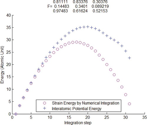
In Figures 2–4, it is seen that the interatomic potential are identical to the strain energy obtained through numerical integration of atomistic stress–strain pair. In each of the three cases, the initial atomic configuration and deformation gradient are randomly created. It is numerically verified again in Figure 5 that Hencky strain is not conjugate to atomic Kirchhoff stress. The number of atoms, , used in Figures 2–4 is 10. Actually it was numerically verified that the conclusion about conjugacy is independent of . Also, as an observation, the conjugacy is valid regardless whether the atoms are in their equilibrium position, i.e. work conjugacy is independent of initial stress or initial potential energy.

Figure 2. Interatomic potential energy compared with strain energy calculated by the atomistic first-order Piola–Kirchhoff stress and deformation gradient , verified by using Tersoff potential.

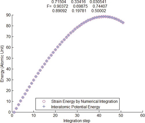
Figure 3. Interatomic potential energy compared with strain energy calculated by the atomistic second-order Piola–Kirchhoff stress and Lagrangian strain , verified by using Tersoff potential.

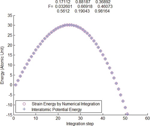
Figure 4. Interatomic potential energy compared with strain energy calculated by the atomistic Kirchhoff stress and Logarithmic strain , verified by using Tersoff potential.

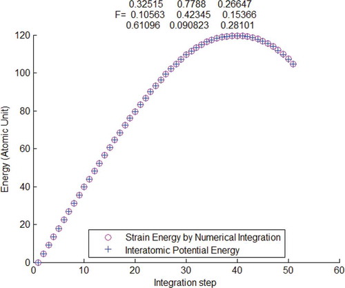
Figure 5. Interatomic potential energy compared with strain energy calculated by the atomistic Kirchhoff stress and Hencky strain , verified by using Tersoff potential.

In Table 2, we summarize the conjugacy verification of atomistic stress and strain in case of pair potential. The interatomic potential adopted here are Coulomb–Buckingham, Lennard–Jones potential and an artificial created interatomic potential.

Table 2. Conjugacy verification of atomistic stress strain pair in pair potential case.

Pair potential case	Atomistic stress for pair potential	Atomistic strain	Conjugacy verification
PK1 2nd form/deformation gradient
PK1 3rd form/deformation gradient
PK2 2nd form/Lagrangian strain
PK2 3rd form/Lagrangian strain
Kirchhoff stress 2nd form /logarithmic strain
Kirchhoff stress 3rd form(Virial)/logarithmic strain

Also, in case of pair potential, it is numerically verified that

(84)

(85)

(86)

Thus, in summary, it is concluded that the strain energy calculated from the conjugate pair of atomistic stress and strain (cf. Tables 1 and 2) equals to the interatomic potential energy for any given arbitrary deformation gradient and initial atomic configuration, i.e.

(87)

6. Conclusion and discussion

The atomistic first-order Piola–Kirchhoff stress is analytically obtained through work conjugate relation with deformation gradient. It is numerically verified that, for both pair potential and three-body potential, the atomistic first-order Piola–Kirchhoff stress , atomistic second-order Piola–Kirchhoff stress and atomistic Kirchhoff stress are conjugates to deformation gradient , Lagrangian strain and logarithmic strain respectively. The conjugacy for atomistic Kirchhoff stress and logarithmic strain is valid when deformation gradient has all positive eigenvalues, otherwise the logarithmic strain is not defined. For all other pairs of atomistic stress and strain, the only requirement for conjugacy is that the deformation gradient is real-valued. Hencky strain is not conjugate to any atomistic stress [18]. The conjugate atomistic stress and strain pair yields interatomic potential energy upon integration. It is noticed that the virial stress at 0 K based on the original volume is a special form of atomistic Kirchhoff stress for pair potential; virial stress based on the current volume is a special form of atomistic Cauchy stress.

In this work, the atomistic system used to calculate stress and strain involves all existing atoms. In the real-world application, a region has to be defined in order to calculate the stress and strain of the atoms within. A system may have several regions and may be much larger than the region specified. How to treat the atoms outside of the region and how to calculate the atomistic stress rigorously remain as an open question.

Disclosure statement

No potential conflict of interest was reported by the authors.

Additional information

Notes on contributors

Leyu Wang

Leyu Wang is a research assistant professor at the Center for Collision Safety and Analysis, George Mason University. He received his PhD degree in mechanical engineering from the George Washington University in 2015. His research interests include fracture mechanics, solid mechanics, molecular dynamics, multi-scale modeling, dynamic finite element analysis, material constitutive modeling, and automobile safety.

James D. Lee

James D. Lee is a professor in the Department of Mechanical and Aerospace Engineering, George Washington University since 1990. He is a fellow of ASME. He received his PhD from Princeton University in 1967. Since then, he has been teaching and/or doing research in universities (Purdue U., West Virginia U., U. of Akron, U. of Minnesota and GWU), industry (The General Tire and Rubber Company), and US government laboratories (NIST and NASA). His research fields include liquid crystals, fracture mechanics, composite materials, optimal control theory, robotics, finite element and meshless methods, molecular dynamics, biomechanics, and microcontinuum physics. Most recently, he has been doing research on multiple time/length scale modeling from atoms to continua. He has been a principal investigator of research grants awarded by NASA, NSF, and US DOT. He has published two books and more than 120 journal articles.

Cing-Dao Kan

Cing-Dao Kan received his PhD degree in Mechanical Engineering from University of Maryland in 1990. He joined George Mason University in May 2013 as Professor of Computational Solid Mechanics in the College of Science. At George Mason he serves as the Director of the newly founded Center for Collision Safety and Analysis (CCSA). Previously, Dr Kan worked at The George Washington University for more than 20 years. He served as the Director of the National Crash Analysis Center (NCAC) from July 2005 to May 2013. His research activities have been focused on computational solid mechanics using nonlinear finite element (FE) modeling and analysis methodologies. While at NCAC he led efforts to develop vehicle structural and occupant models, conduct evaluations of vehicle crashworthiness, assess bumper-height compatibility issues in collisions between large and small vehicles, analyze roadside hardware safety, and conduct component and full-scale crash tests to gather data for formulating models and/or validating simulation results.

Dr Kan was a pioneer in research on the implementation of the nonlinear explicit FE code on high-performance parallel computer platforms. His research and development efforts in benchmarking of high-performance computing platforms for crash simulations have become standards used today in the automotive industry. Under his leadership the NCAC landed multimillion dollar contracts that involved more than 60 task orders for testing, modeling building and validations, analysis of highway barrier crashworthiness, vehicle safety, occupant risk analysis, outreach programs, and crash information management.

Appendix 1.

Remark on the objectivity of logarithmic strain and Hencky strain

In this appendix, a MATLAB® Code is presented to show that Hencky strain, logarithmic strain and asymmetric logarithmic strain are objective tensor quantities with respect to Galilean transformation [31] and they are not equal to each other in general.

Because the reference Lagrangian configuration is affected by the change of the frame of the Eulerian coordinate, the Galilean objectivity of deformation gradient as defined [31,32].

where is a time independent transformation matrix. Notice that the deformation gradient should reduce to identity matrix at the initial undeformed stage, therefore the Lagrangian and Eulerian coordinates are essentially related. The same formula is also derived by Murdoch with different methodology [33].

First, we polar decompose the deformation gradient as [34]

where is the left stretch tensor; is the right stretch tensor; is the rotational matrix with . It leads to

The eigenvalue decomposition is performed on

where

are the three eigenvalues; are the three corresponding eigenvectors . One may define

Then the left stretch tensor and the Hencky strain are calculated as

where the operation ‘’ is defined in Equations (7)–(10).

If the Hencky strain is Galilean objective, the following equation should be valid.

(A1)

where , and stand for the Hencky strain, left stretch tensor and deformation gradient, respectively, in the transformed Eulerian coordinate.

Similarly, the asymmetric Logarithm is Galilean objective if the following equation is valid

(A2)

where is the asymmetric logarithmic strain in the transformed Eulerian coordinate and the operation ‘’ is defined in Equation (7)–(11).

The logarithmic strain as defined in Equation (13) is Galilean objective if the following equation is valid.

(A3)

It is noticed that, in general

(A4)

The following is a MATLAB® code, which enables one to prove numerically that Hencky strain, logarithmic strain, asymmetric logarithmic strain are objective.

function HenckyObjective clear;clc; F = rand(3,3); %random deformation gradient (3X3) alpha = rand; %rotational angle about x axis beta = rand; %rotational angle about y axis gama = rand; %rotational angle about z axis Rx = [1 0 0; 0 cos(alpha) -sin(alpha); 0 sin(alpha) cos(alpha)]; %Rotational matrix of x Ry = [cos(beta) 0 sin(beta); 0 1 0; -sin(beta) 0 cos(beta)];%Rotational matrix of x Rz = [cos(gama) -sin(gama) 0; sin(gama) cos(gama) 0; 0 0 1];%Rotational matrix of x Q = Rx*Ry*Rz; %random transformation matrix %FF is Deformation gradient F in the transformed coordinates FF = Q*F*Q’; %Galilean Objectivity: F* = QFQ %FF = Q*F; %Classic objective: F* = FQ %Verify Hencky Strain [R U V] = pol(F); H = logm2(V); [RR UU VV] = pol(FF); HH = logm2(VV); ‘Hencky is objective if value ~ = 0ʹ Q’*HH*Q-H %% Equation A3.1 Verified %Verify Asymmetric Logarithmic Strain D = logm2(F); %Asymmetric logarithmic strain in the original coordinates DD = logm2(FF); %Asymmetric logarithmic strain in the transformed coordinates ‘Asymmetric Atomic Logarithmic Strain is objective if value ~ = 0’ Q*D*Q’-DD %% Equation A3.2 Verified %Verify Logarithmic Strain L = zeros(3,3); LL = zeros(3,3); for i = 1:3 for j = 1:3 L(i,j) = 1/2*(D(i,j)+D(j,i)); LL(i,j) = 1/2*(DD(i,j)+DD(j,i)); end end ‘Logarithmic Strain is objective if value ~ = 0ʹ Q’*LL*Q-L %% Equation A3.3 Verified % ‘Hencky is equivalent to Logarithmic strain value ~ = 0ʹ H-L %% Equation A3.4 Verified ‘Hencky is equivalent to Asymmetric Logarithmic strain value~ = 0ʹ H-D %% Equation A3.4 Verified ‘Asymmetric Logarithmic strain is equals to logarithmic strain if value~ = 0ʹ L-D %% Equation A3.4 Verified end function [R U V] = pol(F) % F = RU = VR R’ = inv(R) VV = F*F’; [Q LL] = eig(VV); L = LL.^0.5; V = Q*L*Q’; R = inv(V)*F; U = inv(R)*F; end function [A] = logm2(F) % Matrix log, same as MATLAB ‘logm’ [V,D] = eig(F); logD = zeros(3,3); for i = 1:1:3 logD(i,i) = log(D(i,i)); end A = V*logD*inv(V); end

Appendix 2.

Tersoff potential

The Tersoff potential may be expressed as [28]

where

Note that

The atomistic forces can be obtained as

which implies

.

where

.

It is seen that , which implies, among any three atoms, , Tersoff potential yields

Thus it is proved that in general

Appendix 3.

Remark on virial stress

In the study of stress tensors in atomic scale, one frequently encounters a question: is atomistic Kirchhoff stress equal to virial stress ? In this Appendix, we utilize MATLAB® to show that there is a condition, that is has to be parallel to . If so, then . The MATLAB® code is attached herewith.

%The following is the MATLAB® code. clear clc R = rand(3,1); FA = rand(3,3); r = FA*R; f = rand(3,1); test1 = r*f’-f*R’*FA’ f = rand*r; %This is the condition that f parallel to r test2 = r*f’-f*R’*FA’ %‘test1’ is not zero indicates the equation does not hold when r and f is in arbitrary direction. %‘test2’ is zero indicates the equation holds if r is parallel to f.

Appendix 4.

MATLAB® code that numerically verify the conjugacy

Some of the conclusions and observations in this work are obtained through numerical simulations. Therefore, for interested readers to verify, cross exam or to apply for new examples, it is important and useful to have the access to the MATLAB® code, which verifies the conjugacy of atomistic stress–strain pairs as listed in Tables 1 and 2. Three-body Tersoff potential, two-body Lennard Jones potential, Coulomb Buckingham potential and an artificially created potential may be used to verify the conjugacy. The deformation gradient and the initial positions of atoms are randomly generated. All atoms follow a single-valued deformation gradient. Numerically integration is adopted to calculate the strain by dividing the deformation process into multiple small steps. The interatomic potential and the strain energy of each step are calculated. The result shows an exact match between the interatomic potential and the strain energy calculated by the specified conjugate pair (cf. Equation (81)).

% % Below is the MATLAB Code function []=conjugate4() clear;clc;close all % % This MATLAB Code numerically verified the conjugacy between % atomic stress and strain pairs with Tersoff, Lennard Jones and % Coulomb Buckingham Potential. Strain is calculated from a % single displacement gradient for all atoms and is consider uniform % within the volume. Stress is defined on a group of atoms. % Unit is atomic unit. % Written by Leyu Wang, James Lee on 05/04/2016. All rights reserved. % Please cite the associated paper % Leyu Wang, James D. Lee, Cing-Dao Kan, % “Work Conjugate Pair of Stress and Strain in Molecular Dynamics” % International Journal of Smart and Nano Materials % Volume X, Issue X, 2016 % http://dx.doi.org/10.1080/19475411.2016.12331

sw1=1;%set sw1 to chose the atomistic stress/strain pair to be verified %sw1=31 PK1(Truesdell) General Form(fxX)/Deformation Gradient(Conjugate) %sw1=311 PK1(Erigen)/Deformation Gradient(Not Conjugate) %sw1=7 PK1 2nd Form(Pair Potential)/Deformation Gradient(Conjugate) %sw1=3 PK1 3rd Form(Pair Potential)/Deformation Gradient(Conjugate)

%sw1=32 PK2 General Form(fxr)/Lagrangian Strain(Conjugate) %sw1=321 PK2 General Form(rxf)/Lagrangian Strain(Conjugate) %sw1=8 PK2 2nd Form (Pair Potential)/Lagrangian Strain(Conjugate) %sw1=2 PK2 3rd Form (Pair Potential)/Lagrangian Strain(Conjugate)

%sw1=33 Kirchhoff Stress General Form/Logarithmic Strain(Conjugate) %sw1=331 Kirchhoff Stress General Form/Logarithmic Strain(Conjugate) %sw1=332 Kirchhoff Stress General Form/Logarithmic Strain(Conjugate) %sw1=11 Kirchhoff 2nd Form (Pair Potential)/Logarithmic Strain(Conjugate) %sw1=1 Kirchhoff 3rd Form (Virial Stress)(Pair Potential)/Logarithmic % Strain(Conjugate)

sw2=1; %set sw2 to chose the interatomic potential %sw2=1 to use Coulomb-Buckingham potential %sw2=2 to use Lennard-Jones Potential %sw2=3 to use artificial non-linear spring %sw2=777 to use Tersoff potential %Caution: 2-body potential stress should not be used if three body Tersoff %is in use (sw2=1 requires % sw1=31,331,32,321,33,331,332)

sw3=1; %set sw3 to determine the integration step %sw3=1 to user linear integration step %sw3=2 to use nonlinear integration step (1st form) %sw3=3 to use nonlinear integration step (2nd form)

sw4=1; %set sw4 to determine which strain is used when stress is Kirchhoff %stress (sw1=33,331,332,11,1) %sw4=1 logarithmic strain: L=1/2(logm2(F)+logm2(F)’) %sw4=2 asymmetric logarithmic strain: Lhat=logm2(F) %sw4=3 Hencky strain: F=RU=VR; H=logm2(V)% Not Conjugate anum=10; % number of random generated atoms dstep=177;% number of numerical integration steps % more steps, better convergence if sw3>1;dstep=7777;end; % larger dstep for non-linear steps(sw3=2,3) X=randn(3,anum) /25;% Original position of atoms (randomly generated) q=randn(1,anum); % randomly generated electric charge for i=1:1:length(q) if q(i)>(1/2) q(i)=-1; else q(i)=1; end end A=0.3;% Coulomb-Buckingham Potential Parameter B=0.2;% Coulomb-Buckingham Potential Parameter C=0.5;% Coulomb-Buckingham Potential Parameter e=0.15;%Coulomb-Buckingham Potential Parameter anum=(length(X(1,:)));% total number of atoms epsl=0.15 ;% Coulomb-Buckingham parameter sigma=2.5e-2;% Coulomb-Buckingham parameter volume=1.2;% Volume of unit cell x=zeros(3,anum);% coordinate of the deformed atoms r=zeros(3);%relative potions vector of each j atom regards to an i atom rs=0; % scalar value of r f=zeros(3,1);% force vector of each j atom regards to a specific i atom fs=0; % scalar value of f strain=zeros(3,3);% “Hencky-like” strain laststrain=zeros(3,3);% “Hencky-like” strain of last deformation step laststress=zeros(3,3);% virial stress of last deformation step AA=zeros(3,3);% matrix used to make “Hencky-like” strain symmetry BB=zeros(3,3);% matrix used to make “Hencky-like” strain symmetry StrainE=zeros(1,dstep); % “Hencky-like” strain of each integration step PotentialE=zeros(1,dstep); % Potential energy of each integration step V=0;% Interatomic Potential Energy(absolute value) ECM=0;% Strain Energy(absolute value) ct=0; % logical control switch to determine the first deformation step FA=zeros(3,3);% deformation gradient % F=rand(3,3); % Randomly generate a deformation gradient FA which satisfy: [aa bb]=eig(F);% All three Eigen values of deformation gradient are positive while bb(1,1)<0 || bb(2,2)<0 || bb(3,3)<0 F=rand(3,3); [aa bb]=eig(F); end if 0 % set to 1,set sw1 = 1,11,31 and compare the stress value to verify F =[0.0915 0.1123 0.6035%the equivalent of 1 11 31 for two body potential 0.4053 0.7844 0.9644 0.1048 0.2916 0.4325] X =[0.0073 -0.0510 0.0031 -0.0351 -0.0077 -0.0300 -0.0212 0.0655 0.0794 -0.0215 -0.0211 0.0279 0.0321 -0.0632 -0.0312 -0.0457 0.0185 0.0514 -0.0150 0.0243 -0.0297 -0.0179 0.0511 0.0080 0.0223 0.0352 -0.0426 0.0337 -0.0303 0.0393]’ q =[1 -1 1 -1 -1 -1 1 1 1 1] end % if sw2==777&&(sw1==7||sw1==3||sw1==8||sw1==2||sw1==11||sw1==1) z=[‘The selected stress is only valid for pair potential. Please ‘…‘ use 2-body stress(sw1==7,3,8,2,11,1)with 2-body potential(sw2=1,2,3)’…‘ If general 3-body stress is chosen(sw1=31,32,321,33,331,332)’…‘ interatomic potential can be anything(sw2=1,2,3,777’] return end % for c=0:1/dstep:1 % c is the scale factor range from 0~1 to scale FA ct=ct+1;% c=0 FA=I;c=1 FA=F % calculate deformation gradient FA of current integration step if sw3==1; FA=(F-[1 0 0;0 1 0;0 0 1])*c+[1 0 0;0 1 0;0 0 1]; end; if sw3==2; %This verified the nonlinear step also proves the conjugacy FA=(F-[1 0 0;0 1 0;0 0 1])*(sin(c*3*pi)*exp(c-1)/exp(-1))+[1 0 0;0 1 0;0 0 1]; end; if sw3==3; %This verified the nonlinear step also proves the conjugacy FA=(F-[1 0 0;0 1 0;0 0 1])*exp(c-1)/exp(-1)+[1 0 0;0 1 0;0 0 1]; end; for i=1:1:anum % X: original position of atoms x(:,i)=FA*X(:,i);% x: current position of atoms end V=0;% Interatomic Potential stress=0;% stress strain=0;% strain if sw2==777 && (sw1==31||sw1==32||sw1==33||sw1==311||sw1==321||sw1==331||sw1==332) [ff,V]=tersoff(X’,x’); %ff: force V: interatomic Potential for i=1:1:anum f=ff(i,:)’; RX=X(:,i); rx=x(:,i); if sw1==31;stress=stress-f*RX’/1/volume ; end; if sw1==311; stress=stress-RX*f’/1/volume ; end; if sw1==32;stress=stress+(-inv(FA)*f*RX’/1/volume); end; if sw1==321; stress=stress+RX*((-inv(FA)*f)’/1/volume); end; if sw1==33;stress=stress+(-f*rx’/volume); end; if sw1==331; stress=stress+(-rx*f’/volume); end; if sw1==332; stress=stress-f*RX’*FA’/1/volume; end; end else %% if two body potential is used for i=1:1:anum fsumj=[0;0;0]; for j=1:1:anum if i~=j r=x(:,i)-x(:,j); % Calculate relative position vector r rx=x(:,i); rs=norm(r); R=X(:,i)-X(:,j); RX=X(:,i); RS=norm(R); if sw2==1;%Coulomb Buckingham force fs=-1*((6*C)/rs^7-(A*B)/exp(B*rs)-(q(i)*q(j))/(2*pi*e*rs^2)); end if sw2==2;%Lennard Jones force fs=-4.*epsl.*(-12.*sigma.^12*rs.^(-13)+6.*sigma.^6.*rs.^(-7)); end if sw2==3%Artifical Potential Force fs=-1*(exp(rs) + 13311976018446917659705292704529…. /(40564819207303340847894502572032*rs^(2959448103794363…. /4503599627370496)) + 17761006055167241326235515960117…. /(81129638414606681695789005144064*rs^(5917677560790051…. /9007199254740992)) + 3451862223852193902130508091051…. /(20282409603651670423947251286016*rs^(1925733552874571…. /9007199254740992))); end f=fs.*r./norm(r); fsumj=fsumj+f; % summation force act on i-th atom by all j-th atom % Stress Calculation if sw1==7 % PK1 2nd form(Pair Potential)/Deformation Gradient stress=stress-f*R’/2/volume end if sw1==3 % PK1 3rd form(Pair Potential)/Deformation Gradient stress=stress+(-(r*(f)’)*inv(FA)’/2/volume); end if sw1==8 % PK2 2nd Form (Pair Potential)/Lagrangian Strain stress=stress-inv(FA)*f*R’/2/volume end if sw1==2 % PK2 3rd form (Pair Potential)/Lagrangian Strain stress=stress+(-inv(FA)*(r*(f)’)*inv(FA)’/2/volume); end if sw1==11% Kirchhoff Stress 2nd form (Pair Potential)/Logarithmic Strain stress=stress+(-f*r’/2/volume); end if sw1==1 % Kirchhoff Stress 3rd form (Pair Potential)(Virial Stress)/Log Strain stress=stress+(-r*f’/2/volume); end % Interatomic Potential Energy Calculation if sw2==1 %Coulomb Buckingham Potential V=V+(A/exp(B*rs) - C/rs^6 + (q(i)*q(j))/(2*pi*e*rs))/2; end if sw2==2 %Lennard Jones Potential V=V+ (4.*epsl.*(sigma.^12.*rs.^(-12)-sigma.^6.*rs.^(-6)))./2; end if sw2==3 %Artificial Potential V=V+(exp(rs) + (487450249592031*rs^(7081465701866421/9007199254740992…. ))/2251799813685248 + (5748788263873337*rs^(3089521693950941/…. 9007199254740992))/9007199254740992 + (8620900096395613*rs^…. (1544151523576133/4503599627370496))/9007199254740992)/2; end end end if sw2~=777&&(sw1==31||sw1==32||sw1==33||sw1==311||sw1==321||sw1==331||sw1==332) f=fsumj; RX=X(:,i); rx=x(:,i); if sw1==31;stress=stress-f*RX’/1/volume;end; if sw1==311; stress=stress-RX*f’/1/volume;end; if sw1==32;stress=stress+(-inv(FA)*f*RX’/1/volume);end; if sw1==321; stress=stress+RX*((-inv(FA)*f)’/1/volume);end; if sw1==33;stress=stress+(-f*rx’/volume);end; if sw1==331; stress=stress+(-rx*f’/volume);end; if sw1==332; stress=stress-f*RX’*FA’/1/volume;end; end end end % % Strain Calculation % if sw1==31||sw1==311||sw1==7||sw1==3 strain=FA; end if sw1==32||sw1==321||sw1==8||sw1==2 strain=1/2*(FA’*FA-eye(3,3)); end if sw1==33||sw1==331||sw1==332||sw1==11||sw1==1 if sw4==1 AA=logm2(FA); for ii=1:3 %keep only the symmetric part of logm2(FA) for jj=1:3 BB(ii,jj)=1/2*(AA(ii,jj)+AA(jj,ii)); end end strain=BB; end if sw4==2 strain=logm2(FA); end if sw4==3% Hencky Strain; Not conjugate to any stress [RA UA VA]=pol(FA); HA=logm2(VA); strain=HA; end end % % Calculate strain energy by numerical integration % for a=1:3 for b=1:3 ECM=ECM+1/2*(stress(a,b)+laststress(a,b))*(strain(a,b)-laststrain(a,b)); end end if ct==1% save the initial strain energy and interatomic potential energy ECM0=ECM ; EMD0=V ; end laststress=stress; laststrain=strain; StrainE(ct)=(ECM-ECM0)*volume; % Relative stain energy by subtract the value of 1st step PotentialE(ct)=V-EMD0; % Relative interatomic potential energy by subtract the value of 1st step end % % plot relative interatomic potential and relative strain energy % of each integration step % figure2 = figure(‘Color’,[1 1 1]); hold on tt=num2str(F); tt=[‘ ‘,tt(1,:);’F= ‘,tt(2,:);’ ‘,tt(3,:)]; title(tt) plot(real(StrainE)’,’mo’,’MarkerSize’,7) plot(PotentialE’,’b+’,’MarkerSize’,7) legend(‘Strain Energy by Numerical Integration’,…. ‘Interatomic Potential Energy’,’Location’,’Best’) xlabel(‘Integration step’) ylabel(‘Energy (Atomic Unit) ‘) stress strain end function [A] = logm2(F)% F=RU=V; R is rotational matrix; R’=inv(R) [V,D] = eig(F); logD=zeros(3,3); for i=1:1:3 logD(i,i)=log(D(i,i)); end A=V*logD*inv(V); end

function [R U V] = pol(F)% F=RU=VR R’=inv(R) VV=F*F’; [Q LL]=eig(VV); L=LL.^0.5; V=Q*L*Q’; R=inv(V)*F; U=inv(R)*F; end % % Tersoff Potential % function [fatomtemp,engpot]=tersoff(X,x) anum=max(size(X)); xatom=X; uatom=x-X; engpot=0; atompot=zeros(anum,1); fatomtemp=zeros(anum,3); f2ij=zeros(3,1); %==================================================================== ri=zeros(3,1); rj=zeros(3,1); rk=zeros(3,1); tij=zeros(3,1); tik=zeros(3,1); f2ij=zeros(3,1); f3ij=zeros(3,1); f3ik=zeros(3,1); f3i=zeros(3,1); f3j=zeros(3,1); f3k=zeros(3,1); pram=zeros(11,1); pram(1)=1.3936d3*0.03674932587; pram(2)=3.467d2*0.03674932587; pram(3)=3.4879/1.889726134d0; pram(4)=2.2119/1.889726134d0; pram(5)=1.5724d-7; pram(6)=0.72751d0; pram(7)=3.8049d4; pram(8)=4.384d0; pram(9)=-.57058d0; pram(10)=1.8*1.889726134d0; pram(11)=2.1*1.889726134d0; %==================================================== uvol=1.0d0; factor=1.0d0/uvol; %==================================================== for iatom=1:1:anum kia=1; % carbon parameters ai=pram(1,kia); bi=pram(2,kia); aai=pram(3,kia); bbi=pram(4,kia); betai=pram(5,kia); eni=pram(6,kia); eni1=eni-1.0d0; eni2=-0.5d0/eni-1.0d0; eni3=-0.5d0/eni; ci=pram(7,kia); di=pram(8,kia); hi=pram(9,kia); rri=pram(10,kia); si=pram(11,kia); %==================================================== ri(1)=xatom(iatom,1)+uatom(iatom,1); ri(2)=xatom(iatom,2)+uatom(iatom,2); ri(3)=xatom(iatom,3)+uatom(iatom,3); %==================================================== %==================================================== %==================================================== for jatom=1:1:anum if jatom==iatom continue%ignor the rest of the code for this loop end kja=1; % carbon parameters aj=pram(1,kja); bj=pram(2,kja); aaj=pram(3,kja); bbj=pram(4,kja); rrj=pram(10,kja); sj=pram(11,kja); %==================================================== aij=sqrt(ai*aj); bij=sqrt(bi*bj); aaij=0.5d0*(aai+aaj); bbij=0.5d0*(bbi+bbj); rrij=sqrt(rri*rrj); sij=sqrt(si*sj); rj(1)=xatom(jatom,1)+uatom(jatom,1); rj(2)=xatom(jatom,2)+uatom(jatom,2); rj(3)=xatom(jatom,3)+uatom(jatom,3); t1=ri(1)-rj(1); t2=ri(2)-rj(2); t3=ri(3)-rj(3); rij=sqrt(t1*t1+t2*t2+t3*t3); if(rij>sij) continue%ignor the rest of the code for this loop end tij(1)=t1/rij; tij(2)=t2/rij; tij(3)=t3/rij; %================================================== % calculate attractive and repulsive energy terms %================================================== vaij=aij*exp(-aaij*rij); vrij=bij*exp(-bbij*rij); [fcij,dfcij]=fc(rij,rrij,sij); %================================================== % calculate third-body parameters %================================================== %==================================================== %==================================================== gxij=0.0d0; for latomt=1:1:anum%500 if(latomt==iatom)||(latomt==jatom) continue end kka=1; rrk=pram(10,kka); sk=pram(11,kka); %------------------------------------------ rrik=sqrt(rri*rrk); sik=sqrt(si*sk); %==================================================== %==================================================== rk(1)=xatom(latomt,1)+uatom(latomt,1); rk(2)=xatom(latomt,2)+uatom(latomt,2); rk(3)=xatom(latomt,3)+uatom(latomt,3); t1=ri(1)-rk(1); t2=ri(2)-rk(2); t3=ri(3)-rk(3); rik=sqrt(t1*t1+t2*t2+t3*t3); if(rik>sik) continue end tik(1)=t1/rik; tik(2)=t2/rik; tik(3)=t3/rik; [fcik,dfcik]=fc(rik,rrik,sik); %============================================================ %calculatekxi=fc(rik)g(theta) %============================================================ cost=tij(1)*tik(1)+tij(2)*tik(2)+tij(3)*tik(3); gtheta=1.0d0+(ci/di)^2-ci^2/(di^2+(hi-cost)^2); gxij=gxij+fcik*gtheta; end %500 %==================================================================== % calculate bond-factor bfij={1+(bi*kxi)^eni}^(-0.5/ni)and force coefs %==================================================================== temp1=betai*gxij; if(temp1<0.0d0) temp2=1.0d0; bfij=1.0; coef1=0.0d0 ; else; temp2=1.0d0+temp1^eni; bfij=temp2^eni3; coef1=0.5d0*betai*temp1^eni1*temp2^eni2*fcij*vrij; end %==================================================================== %potential energy engtersoff=fcij*(vaij-bfij*vrij)/2.0d0; engpot=engpot+engtersoff; atompot(iatom)=atompot(iatom)+engtersoff; %==================================================================== %calculate two-body forces %==================================================================== fij=-0.5d0*(vaij*(dfcij-fcij*aaij)-bfij*vrij*(dfcij-fcij*bbij)); %==================================================================== fijx=fij*tij(1); fijy=fij*tij(2); fijz=fij*tij(3); %==================================================================== fatomtemp(iatom,1)=fatomtemp(iatom,1)+fijx; fatomtemp(iatom,2)=fatomtemp(iatom,2)+fijy; fatomtemp(iatom,3)=fatomtemp(iatom,3)+fijz; fatomtemp(jatom,1)=fatomtemp(jatom,1)-fijx; fatomtemp(jatom,2)=fatomtemp(jatom,2)-fijy; fatomtemp(jatom,3)=fatomtemp(jatom,3)-fijz; %==================================================================== f2ij(1)=fijx; f2ij(2)=fijy; f2ij(3)=fijz; %--------------------------------------------------------------------- % for ic=1:1:3 % for jc=1:1:3 % stressa(ic,jc,iatom)=stressa(ic,jc,iatom)+0.5*factor*f2ij(ic)*(-tij(jc))*rij % stressa(ic,jc,jatom)=stressa(ic,jc,jatom)+0.5*factor*f2ij(ic)*(-tij(jc))*rij % end % end %==================================================================== %==================================================================== for katomt=1:1:anum%3000 if(katomt==iatom)||(katomt==jatom) continue end kka=1;%jtype(katomt); rrk=pram(10,kka); sk=pram(11,kka); rrik=sqrt(rri*rrk); sik=sqrt(si*sk); %==================================================================== rk(1)=xatom(katomt,1)+uatom(katomt,1); rk(2)=xatom(katomt,2)+uatom(katomt,2); rk(3)=xatom(katomt,3)+uatom(katomt,3); t1=ri(1)-rk(1); t2=ri(2)-rk(2); t3=ri(3)-rk(3); rik=sqrt(t1*t1+t2*t2+t3*t3); if(rik>sik) continue end tik(1)=t1/rik; tik(2)=t2/rik; tik(3)=t3/rik; [fcik,dfcik]= fc(rik,rrik,sik); cost=tij(1)*tik(1)+tij(2)*tik(2)+tij(3)*tik(3); gtheta=1.0d0+(ci/di)^2-ci^2/(di^2+(hi-cost)^2); coef2=-fcik*2.0d0*ci^2*(hi-cost)/(di^2+(hi-cost)^2)^2; %==================================================================== %------------------- fkx=0.5d0*coef1*(gtheta*dfcik*tik(1)+coef2*(tij(1)-cost*tik(1))/rik); %------------------- fky=0.5d0*coef1*(gtheta*dfcik*tik(2)+coef2*(tij(2)-cost*tik(2))/rik); %------------------- fkz=0.5d0*coef1*(gtheta*dfcik*tik(3)+coef2*(tij(3)-cost*tik(3))/rik); %------------------- fjx=0.5d0*coef1*coef2*(tik(1)-cost*tij(1))/rij; %------------------- fjy=0.5d0*coef1*coef2*(tik(2)-cost*tij(2))/rij; %------------------- fjz=0.5d0*coef1*coef2*(tik(3)-cost*tij(3))/rij; %==================================================================== fatomtemp(iatom,1)=fatomtemp(iatom,1)-(fkx+fjx); fatomtemp(iatom,2)=fatomtemp(iatom,2)-(fky+fjy); fatomtemp(iatom,3)=fatomtemp(iatom,3)-(fkz+fjz); %==================================================================== fatomtemp(jatom,1)=fatomtemp(jatom,1)+fjx; fatomtemp(jatom,2)=fatomtemp(jatom,2)+fjy; fatomtemp(jatom,3)=fatomtemp(jatom,3)+fjz; %==================================================================== fatomtemp(katomt,1)=fatomtemp(katomt,1)+fkx; fatomtemp(katomt,2)=fatomtemp(katomt,2)+fky; fatomtemp(katomt,3)=fatomtemp(katomt,3)+fkz; %==================================================================== %==================================================================== f3j(1)=fjx; f3j(2)=fjy; f3j(3)=fjz; %------------------- f3k(1)=fkx; f3k(2)=fky; f3k(3)=fkz; %==================================================================== %==================================================================== end %3000 continue end %2000 continue end %1000 continue %==================================================== %==================================================== end %========================================= %=========================================

function [f,df]= fc(r,rr,s) if (r<rr) f=1.0d0; df=0.0d0 ; elseif (r>s) f=0.0d0; df=0.0d0; else arg=pi*(r-rr)/(s-rr); f=0.5d0*(1.0d0+cos(arg)); df=-0.5d0*pi*sin(arg)/(s-rr); end end % End of the MATLAB Code

References

- A.C. Eringen, Mechanics of Continua, American Institute of Physics, New York, 1980.
- J.E. Fitzgerald, A tensorial Hencky measure of strain and strain rate for finite deformations, J. Appl. Phys. 51 (1980), pp. 5111–5115. doi:10.1063/1.327428
- H. Xiao, O.T. Bruhns, and A. Meyers, A natural generalization of hypoelasticity and Eulerian rate type formulation of hyperelasticity, J. Elast. 56 (1999), pp. 59–93. doi:10.1023/A:1007677619913
- H. Xiao and L.S. Chen, Hencky’s elasticity model and linear stress-strain relations in isotropic finite hyperelasticity, Acta Mech. 157 (2002), pp. 51–60. doi:10.1007/BF01182154
- M.J. Buehler and H. Gao, Modeling dynamic fracture using large-scale atomistic simulations, in Dynamic Fracture Mechanics, A. Shukla, ed., World Scientific, Singapore, 2006, pp. 1–68.
- Z. Zhang, X. Wang, and J.D. Lee, An atomistic methodology of energy release rate for graphene at nanoscale, J. Appl. Phys. 115 (2014), pp. 114314. doi:10.1063/1.4869207
- J. Li and J.D. Lee, Reformulation of the Nosé–Hoover thermostat for heat conduction simulation at nanoscale, Acta Mech. 225 (2014), pp. 1223–1233. doi:10.1007/s00707-013-1046-4
- S. Shen and S.N. Atluri, Atomic-level stress calculation and continuum-molecular system equivalence, Comput. Model. Eng. Sci.. 6 (2004), pp. 91–104.
- R.J. Hardy, Formulas for determining local properties in molecular-dynamics simulations: Shock waves, J. Chem. Phys. 76 (1982), pp. 622–628. doi:10.1063/1.442714
- J.A. Zimmerman, E.B. WebbIII, J.J. Hoyt, R.E. Jones, P.A. Klein, and D.J. Bammann, Calculation of stress in atomistic simulation, Model. Simul. Mater. Sci. Eng. 12 (2004), pp. S319–S332. doi:10.1088/0965-0393/12/4/S03
- F. Costanzo, G.L. Gray, and P.C. Andia, On the notion of average mechanical properties in MD simulation via homogenization, Model. Simul. Mater. Sci. Eng. 12 (2004), pp. S333–S345. doi:10.1088/0965-0393/12/4/S04
- P.M. Gullett, M.F. Horstemeyer, M.I. Baskes, and H. Fang, A deformation gradient tensor and strain tensors for atomistic simulations, Model. Simul. Mater. Sci. Eng. 16 (2008), pp. 15001. doi:10.1088/0965-0393/16/1/015001
- D.H. Tsai, The virial theorem and stress calculation in molecular dynamics, J. Chem. Phys. 70 (1979), pp. 1375–1382. doi:10.1063/1.437577
- K.S. Cheung and S. Yip, Atomic-level stress in an inhomogeneous system, J. Appl. Phys. 70 (1991), pp. 5688–5690. doi:10.1063/1.350186
- M. Zhou, A new look at the atomic level virial stress: On continuum-molecular system equivalence, Proc. R. Soc. Math. Phys. Eng. Sci. 459 (2003), pp. 2347–2392. doi:10.1098/rspa.2003.1127
- J. Cormier, J.M. Rickman, and T.J. Delph, Stress calculation in atomistic simulations of perfect and imperfect solids, J. Appl. Phys. 89 (2001), pp. 99–104. doi:10.1063/1.1328406
- R. Clausius, On a mechanical theorem applicable to heat, Philos. Mag. Ser. 40 (4) (1870), pp. 122–127.
- L. Wang, J. Li, and J.D. Lee, Work conjugate strain of virial stress, Int. J. Smart Nano Mater. 7 (2016), pp. 39–51. doi:10.1080/19475411.2016.1162218
- J.L. Ericksen, On the Cauchy—Born rule, Math. Mech. Solids 13 (2008), pp. 199–220. doi:10.1177/1081286507086898
- M. Arroyo and T. Belytschko, An atomistic-based finite deformation membrane for single layer crystalline films, J. Mech. Phys. Solids 50 (2002), pp. 1941–1977. doi:10.1016/S0022-5096(02)00002-9
- H.S. Park, P.A. Klein, and G.J. Wagner, A surface Cauchy–Born model for nanoscale materials, Int. J. Numer. Methods Eng. 68 (2006), pp. 1072–1095. doi:10.1002/nme.1754
- A. Kumar, S. Kumar, and P. Gupta, A Helical Cauchy-Born rule for special cosserat rod modeling of nano and continuum rods, J. Elast. 124 (2016), pp. 81–106. doi:10.1007/s10659-015-9562-1
- I.-S. Liu, Continuum Mechanics, Springer Berlin Heidelberg, New York, 2002.
- A.I. Murdoch, Physical Foundations of Continuum Mechanics, Cambridge University Press, Cambridge, 2012.
- S.-L. Xue, B. Li, X.-Q. Feng, and H. Gao, Biochemomechanical poroelastic theory of avascular tumor growth, J. Mech. Phys. Solids 94 (2016), pp. 409–432. doi:10.1016/j.jmps.2016.05.011
- Y.C. Fung and P. Tong, Classical and Computational Solid Mechanics, Vol. 1, World Scientific Publishing Company, Singapore, 2001.
- S. Nair, Introduction to Continuum Mechanics, Cambridge University Press, Cambridge, 2009.
- J. Tersoff, Empirical interatomic potential for carbon, with applications to amorphous carbon, Phys. Rev. Lett. 61 (1988), pp. 2879–2882. doi:10.1103/PhysRevLett.61.2879
- L. Lindsay and D.A. Broido, Optimized Tersoff and Brenner empirical potential parameters for lattice dynamics and phonon thermal transport in carbon nanotubes and graphene, Phys. Rev. B 81 (2010), pp. 205441. doi:10.1103/PhysRevB.81.205441
- H. Balamane, T. Halicioglu, and W.A. Tiller, Comparative study of silicon empirical interatomic potentials, Phys. Rev. B 46 (1992), pp. 2250–2279. doi:10.1103/PhysRevB.46.2250
- I.-S. Liu, On the transformation property of the deformation gradient under a change of frame, J. Elast. 71 (2003), pp. 73–80. doi:10.1023/B:ELAS.0000005548.36767.e7
- I.-S. Liu, Further remarks on Euclidean objectivity and the principle of material frame-indifference, Contin. Mech. Thermodyn. 17 (2005), pp. 125–133. doi:10.1007/s00161-004-0191-3
- A.I. Murdoch, On objectivity and material symmetry for simple elastic solids, J. Elast. Phys. Sci. Solids. 60 (2000), pp. 233–242. doi:10.1023/A:1011049615372
- Polar Decomposition. Available at http://www.continuummechanics.org/polardecomposition.html. (Accessed 16 June 2016).