Flow velocity and temperature sensing using thermosensitive fluorescent polymer seed particles in water

ABSTRACT

Particle image velocimetry (PIV) is an experimental technique that uses microscale particles as tracers to measure the velocity of a fluid flow. In this paper, we seek to extend this technique to simultaneously measure fluid temperature as well, by employing a novel class of thermosensitive polymer particles. Towards this aim, we designed a process to encapsulate highly fluorescent thermosensitive NBD-AE-co-poly(N-isopropylacrylamide) polymers into optically transparent poly(dimethylsiloxane) particles. These novel PIV particles enable direct measurement of water velocity while serving as temperature probes that increase their fluorescence intensity when the temperature rises above 32 °C. To demonstrate the ability of the particles to simultaneously serve as flow tracers and temperature sensors in water, we examine the flow velocity and temperature in the wake of a heated cylinder in a cross flow. Our results indicate the possibility of extending PIV to afford the spatial and temporal resolution of fluid velocity and temperature gradients in water, with potential application to the study of convection problems from life sciences to engineering.

KEYWORDS:

• Fluorescence sensing
• particle image velocimetry
• temperature sensing

1. Introduction

Particle image velocimetry (PIV) is an experimental technique that employs microscale particles as minimally invasive tracers to measure the velocity of a fluid flow [1,2]. In PIV, the particles are uniformly dispersed within the fluid and a laser is used to selectively illuminate a portion of the flow (typically a thin plane). Sequences of images are recorded using a digital camera and subsequently cross-correlated to determine the average displacement of the particles within small interrogation regions between successive frames. The velocity field of the flow is thus reconstructed.

This technique has been extensively applied in academic and industrial laboratories over the last three decades [1,2]. PIV analyses have been often conducted in the aerospace and automotive industries to study external and internal flows. For example, PIV has been used to investigate the flow in the vicinity of a propeller [3,4] and to study internal combustion of automotive engines [5,6]. PIV has also been employed in civil engineering to study air flows in the vicinity of large structures [7,8], and in environmental fluid mechanics to analyze rivers and coastal flows [9]. Further, PIV has been applied in the life sciences, where it has been utilized to inform the design of microfluidic biosensors [10] and investigate the behavior of biological flows [11,12].

The simultaneous measurement of flow temperature may add fundamental information in several PIV applications, ranging from the design of combustion chambers [13] to the optimization of microelectromechanical [14] and microfluidic devices [15]. In this framework, thermoresponsive particles have been recently used with success in air flows, where thermographic phosphor particles show excellent sensitivity and fast time response for temperatures ranging from 280 to 420 K [16]. However, if we look into the use of these tracers in water environments, their application is limited due to poor solubility [17].

A viable technique for temperature sensing in water has been developed using laser-induced fluorescence of Rhodamine dyes, to detect high and low temperature regions in a Rayleigh-Bernard convection cell [18]. While the dependence of the emission on the temperature may allow for repeatable measurements, the dye emission is strongly influenced by several fluid characteristics, such as composition and pH. Infrared thermography has also been used in combination with traditional PIV for the simultaneous study of flow velocity and temperature in a liquid film [19]. However, the application of this technique to water measurements beyond the free surface is not feasible, due to strong absorption of the infrared radiation by the fluid.

An alternative approach entails the integration of thermochromic liquid crystals with traditional particle tracers in PIV experiments [20]. For example, thermochromic liquid crystals have been proposed to study natural convection within a confined cavity [21] and investigate near-wall coherent structures in a turbulent boundary layer [22]. Despite good temperature resolution, the technology is limited by the low out-of-plane spatial resolution, on the order of several millimeters, and the necessity of complex calibration to obtain accurate measurements [23].

In recent years, thermosensitive and thermochromic polymers have attracted an increasing interest for the design of temperature sensors [24], although their application to PIV is presently untested. For example, thermochromic sensors have been prepared by blending fluorescent organic molecules in polyethylene [25] and poly-lactic acid [26]. Similarly, temperature sensors have been developed from oxygen permeable polymers blended with fluorescent platinum porphyrin [27] and from thermosensitive conductive polymer nanofilms [28]. The integration of thermosensitive polymers in optical devices has also been evaluated, whereby thermosensitive polymers have been used for lining optical fibers [29] and Rhodamine-doped polymers have been integrated in optical resonators for temperature sensing [30].

The optical response of thermosensitive polymers, such as poly(N-isopropylacrylamide) (PNIPAAm), could be tailored by incorporating a fluorescent dye into their structure [31–35]. The fluorescent yield of the dyes used in these applications, such as Rhodamine and Benzofurazan derivatives, presents a strong dependency on the polarity of the local environment [32,34–36]. During the thermodynamic transition at the lower critical solution temperature (LCST) of the polymer, the fluorescence of the dye is substantially increased by the reduced polarity of the chains. This class of polymer temperature sensors is particularly attractive for their hydrophilicity and bio-compatibility, which have been leveraged for thermal analysis of living cells [37–39], and to measure the temperature of nanoparticles for cancer treatment [40].

In this work, we develop novel polymer seed particles for simultaneous measurement of velocity and temperature in water flows. Specifically designed for water environments, the particles are biocompatible and neutrally buoyant. In addition, they can be used in traditional PIV systems without specific upgrades. Particles are prepared using a double emulsion process, where a fluorescent thermosensitive NBD-AE-co-PNIPAAm polymer solution is incorporated within a commercial poly(dimethylsiloxane) (PDMS) matrix.

The fluorescent dye selected for this application is a Nitrobenzofurazan derivative (NBD-AE) which is covalently bonded to the backbone of the PNIPAAm chains [32]. By exploiting the decrease in the microenvironmental polarity in the vicinity of the PNIPAAm chains above LCST, the intensity of the dye fluorescence is increased by two to three orders of magnitude for temperatures above 32 °C [32]. To enable PIV, the fluorescent polymer solution is incorporated in PDMS microparticles. The encapsulation process prevent large scale aggregation of the PNIPAAm-based polymers at high temperatures [34], constraining the aggregation of the chains within the particle, and thereby allowing for continuous measurement of the flow velocity and temperature. To demonstrate the possibility of simultaneous measurement of flow velocity and temperature in PIV experiments, we examine the wake off a heated cylinder in water.

The paper is organized as follows. In Section 2, we describe the process for the preparation of the particles and the PIV apparatus used for our demonstration. In Section 3, we discuss the fluorescence response of the particles as a function of temperature. Therein, we also present our results on simultaneous temperature and velocity measurements within PIV. The article concludes in Section 4 with a summary of its main findings. In the Appendix, we succinctly describe a numerical solution of the flow in the wake of the cylinder that is used for comparison with experimental results.

2. Materials and methods

2.1. Materials

N-Isopropylacrylamide (NIPAM, 97%), Azobisisobutyronitrile (AIBN, 98%), 4-Chloro-7-nitrobenzofurazan (NBD-Cl, 98%), Ethanolamine (EtNH₂, ≥98%), Acryloyl chloride (97%), Sorbitane monooleate (Span 80), Sodium dodecyl sulfate (SDS, 99%), Acetonitrile (ACN, 99.8%), 1,4-Dioxane (99.8%), Dichloromethane (DCM, 99.8%), Ethyl acetate (99.8%), N-hexane (95%), and Tetrahydrofuran (THF, ≥99.9%) are purchased from Sigma-Aldrich (www.sigmaaldrich.com). Sylgard 184 silicone elastomer kit (Part A and Part B) is purchased from Fisher Scientific. Deionized water (resistivity 18.2 MΩ) is used to dissolve the polymer and prepare the emulsions. All chemicals are used as received without further purification.

2.2. Polymers characterization

Nuclear magnetic resonance spectra of the dyes are recorded using a Bruker AV III 500 MHz NMR instrument. Infrared spectra of the polymers are measured via a Thermo-Scientific Nicolet 6700 spectrometer with a Smart iTR module for attenuated total reflectance Fourier transform infrared spectroscopy (ATR-FTIR). The molecular weight of the polymers is determined on a Shimadzu Gel Permeation Chromatograph (GPC) with DMF as the eluent.

2.3. Preparation of fluorescent NBD-AE-co-poly(N-isopropylacrylamide) polymer

Fluorescent NBD-AE dye is prepared following procedures reported in the literature [32,41]. NBD-Cl (200 mg) is dissolved in 40 ml ACN. EtNH₂ (200 µl) is added to 10 ml ACN. The EtNH₂ solution is added dropwise to the dye solution while stirring. The mixture is left to react for 30 minutes at room temperature. Products are extracted under reduced pressure and chromatographed on silica gel using DCM:Methanol (20:1) as the eluent to obtain 4-(2-Hydroxyethylamino)-7-nitro-2,1,3-benzoxadiazole (NBD-NHCH₂CH₂OH, ¹H NMR, 500 MHz, DMSO-d₆, δ 3.56 (2H, br), 3.69 (2H, t), 6.47 (1H, d), 8.53 (1H, d)).

NBD-NHCH₂CH₂OH (50 mg) is dissolved in 15 ml ACN, and 1 ml Acryloyl chloride is added to the solution in the reaction flask. The mixture is refluxed for four hours. Reaction products are extracted under reduced pressure and chromatographed on silica gel using ethyl acetate-n-hexane (1:1) to obtain 4-(2-Acryloyloxyethylamino)-7-nitro-2,1,3-benzoxadiazole (NBD-AE, ¹H NMR, 500 MHz, DMSO-d₆, δ 3.82 (2H, m), 4.40 (2H, t), 5.94 (1H, d), 6.16 (1H, m), 6.32 (1H, d), 6.53 (1H, d), 8.54 (1H, d)).

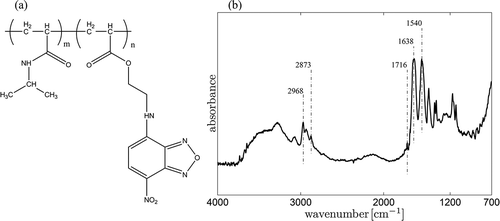
The fluorescent NBD-AE-co-PNIPAAm polymer is prepared by co-polymerizing 0.57 g of NIPAM and 9 mg of NBD-AE in 10 ml of 1,4-Dioxane using 18 mg of AIBN as the thermal initiator. The solution is vacuum-dried and purged with nitrogen five times. After that, the polymerization reaction is conducted for 16 hours at 70 °C under a nitrogen atmosphere. The polymer is extracted under reduced pressure and precipitated in n-hexane from a 5 ml THF solution. The polymer is collected by filtration using Whatman paper and dried under vacuum. The structure of the fluorescent polymer is reported in Figure 1(a). In Figure 1(b), the infrared spectrum recorded for the NBD-AE-co-PNIPAAm polymer confirms the presence of the characteristic absorption peaks of PNIPAAm, located at: 1638 cm⁻¹ and 1527 cm⁻¹ for the C=O and C-N bending vibrations in the amide bond; and at 2873 cm⁻¹ and 2968 cm⁻¹ for the stretching vibrations of the -CH₃ bond [42]. The peak at 1716 cm⁻¹ is attributed to the C=O stretching vibrations in the ester bond of the NBD-AE units.

Figure 1. (a) Structure of the NBD-AE-co-PNIPAAm polymer (m = 157, n = 1). (b) Infrared absorption spectrum of the NBD-AE-co-PNIPAAm polymer.

The weight average molecular weight of the polymer is determined through GPC using a 5 mg/ml solution in DMF as 68.5 kDa with a polydispersity index of 1.93. The dry NBD-AE-co-PNIPAAm polymer is dissolved in deionized water to prepare a 10 mg/ml solution, which is used for the fluorescence experiments and the preparation of the particles.

2.4. Synthesis of thermosensitive particle tracers

The thermosensitive particle tracers are prepared by encapsulating a solution of NBD-AE-co-PNIPAAm in DI water (10 mg/ml) inside a transparent PDMS matrix. The presence of both the fluorescent polymer (NBD-AE-co-PNIPAAm) and the solvent (DI water) inside the PDMS shell is functional to the thermoresponsive fluorescence of the sensors, whereby solubility of PNIPAAm in water is reduced with increasing temperature (at LCST) and the polarity in the vicinity of the chains decreases enhancing emission of the fluorescent units [32].

The particles are fabricated using a water-in-oil-in-water double emulsion process. The main steps of the process are depicted in Figure 2. The PDMS part A (polymer, 5 ml) and part B (crosslinker, 0.5 ml) are added to a 50 ml Falcon cylindrical tube with 0.2 ml of SPAN 80 as the water-in-oil emulsifier. The components are mixed for 2 minutes using a Scientific Industries G560 vortex mixer to prepare a homogenous solution. The water-in-oil emulsion is prepared by adding 1 ml of 10 mg/ml solution of NBD-AE-co-PNIPAAm to the tube and mixing the two phases for 2 minutes using the vortex mixer.

Figure 2. Schematic of the process for preparing the thermosensitive particle tracers.

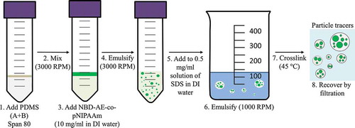
In a glass beaker (400 ml volume, 60 mm inner diameter) equipped with a teflon-coated stirring bar (50 mm length), 0.05–0.1 g of SDS is added to 100 ml deionized water. The water temperature is set to 45 °C and the stirring speed to 1000 rpm. The PDMS water-in-oil emulsion is added dropwise to the water solution containing the SDS emulsifier to prepare the water-in-oil-in-water emulsion. The emulsion is left under continuous stirring for three hours at 45 °C to crosslink the PDMS elastomer by an organometallic crosslinking reaction [43]. Particles with sizes ranging from a few tenths to a few hundred microns are collected by filtration using a Whatman filter for storage and testing¹.

2.5. Fluorescence experiments and particles’ morphology

Fluorescence spectra of the polymer solution and particles suspension are measured using a PTI Quanta Master 40 fluorescence spectrophotometer with 1200 line/mm gratings for emission (400 nm blaze) and excitation (300 nm). A 3.5 ml cuvette with 12.4 mm path length is employed in the experiments. The temperature inside the cuvette is controlled via a Thermo Scientific refrigerated/heated bath circulator. The effective temperature inside the cuvette is measured using an electronic thermometer probe after the temperature in the circulator is stabilized for five minutes.

Optical response of the NBD-AE-co-PNIPAAm polymer as a function of the temperature is investigated by measuring fluorescence emission of a 10 mg/ml solution at temperatures ranging from 14 to 50 °C. In a typical experiment, 3.5 ml of the polymer solution are added to the cuvette using a glass pipette. The cuvette is placed in the test chamber of the spectrophotometer and the temperature is stabilized at 14 °C for five minutes. The spectrum is acquired in the range 500–650 nm with an excitation wavelength of 462 nm. After the acquisition, the temperature in the refrigerated/heated bath circulator is increased using the electronic control to reach the next temperature condition. Temperatures tested are: 14, 20, 28, 31, 32, 35, 39, 43, and 50 °C. For each condition, the temperature is stabilized for five minutes before acquisition of the spectrum.

Fluorescence experiments are repeated after encapsulation of the fluorescent polymers in the PDMS microparticles. The fluorescence-temperature scan is also performed in the range 14 to 50 °C by using a similar setup, whereby the glass cuvette is filled with 3.5 ml of a 50 mg/ml homogeneous suspension of particles in DI water. Fluorescence optical micrographs of the particles are obtained using an Optika B-500TiFL microscope. Scanning electron microscopy (SEM) is performed using a Hitachi S-3400N microscope.

2.6. Apparatus and procedure for PIV experiments

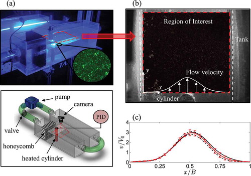
PIV experiments are conducted in an open channel. The experimental apparatus is displayed in Figure 3(a). The apparatus is composed of two rectangular tanks of width B = 100 mm, height H = 150 mm, and length L = 500 mm, with one serving as the test section and the other as a reservoir. The tanks are custom-made from 6.35 mm thick transparent acrylic panels. The test section tank is connected to the reservoir through a recirculation system, with flow generated by a Jebao DC1200 pump. The output of the pump is controlled via a mechanical valve connected in series in the hydraulic circuit. A cylinder is positioned 180 mm downstream from the inlet of the experimental tank in a vertical orientation. A 35 mm thick honeycomb panel with 5 mm cell diameter is positioned 75 mm upstream of the cylinder to minimize velocity fluctuations.

Figure 3. (a) Schematic of the experimental apparatus for the PIV experiment. (b) Image recorded during the PIV experiment. The portion of the image used to determine the velocity vectors is indicated by the red contour (region of interest, ROI). The ROI image is displayed after subtraction of the background image. (c) Normalized velocity in the experimental tank at a depth of 0.625 H without the cylinder: solid black, dashed black, and dashed-dotted black lines are the v component of the velocity at 20, 40, and 60 mm downstream of the cylinder, respectively. The solid red line is the average of the velocities in the three sections.

The cylinder consists of an aluminum tube with an external diameter D = 19 mm and a wall thickness of 1.25 mm². The tube is lined internally with heat transfer paste (MIL-C-47113), and a 405 W cartridge-style immersion heater is lodged inside the tube and fixed using the paste. The external temperature of the cylinder is monitored using via a J-type thermocouple, glued at a nominal height of 0.65 H on the external surface of the cylinder facing the fluid flow. The temperature control is performed using an Extech 96VFL Proportional-Integral-Derivative (PID) controller connected to the thermocouple and the heater. The system is powered through a 120 V power line. The upstream flow temperature is verified by disconnecting the heater and measuring the temperature on the surface of the cylinder using the thermocouple.

Two different experimental conditions are realized by modifying the velocity upstream from the cylinder using the valve. The components of the upstream velocity are determined in the absence of the cylinder using the PIV analysis discussed in Section 2.7. With respect to the coordinate system shown in Figure 3(b), u is the velocity component along the x-direction and v is along the y-direction. The nominal velocity V₀ is computed from the v component of the velocity, shown as the red line in Figure 3(c), by taking its average between x/B = 0 and x/B = 1. The conditions tested in the PIV experiments are V₀ = 15.3 mm/s and 30.7 mm/s; the upstream flow temperature does not exceed 28 °C during the experiments. During the experiments, the flow depth is 0.84 H and the measurement plane is located at 0.625 H.

Analysis of Figure 3(c) suggests that the flow in the tank is laminar, yet non uniform along the width of the channel. By observing the flow velocities at different depths, not shown here for brevity, we assess the presence of a three-dimensional velocity distribution in the tank. In particular, we observe a consistent decrease of the flow velocity close to the bottom of the tank (below 0.3 H).

Temperature sensing using the fluorescent particles is evaluated in two different conditions for each upstream flow velocity. In the first condition, the cylinder is kept at room temperature (approximately 20 °C), while in the second condition the temperature on the surface of the cylinder is set to 60 °C using the PID control.

The flow is seeded using a preparation of 10 g fluorescent particles for approximately 12 liters of tap water. To prevent aggregation of the particles, 4 g of SDS surfactant is added to the fluid. The addition of such a small volume fraction of the surfactant in water is assumed not to affect the dynamic or thermodynamic characteristics of the fluid in this experiment. The ability of the particles to follow the flow past the cylinder is assessed by evaluating the Stokes number [1], based on the cylinder diameter and nominal upstream velocity,

(1)

where d is the diameter of the particle and ν = 10^–6 m²/s is the kinematic viscosity of water at room temperature. For particles of size 20–200 µm, St ranges from 0.006 to 0.090, which is within the typical range of particle tracers for PIV experiments [1]³.

2.7. Image acquisition and processing for PIV experiments

The PIV apparatus comprises a FLEA FL3-U3-13E4C-C camera with a 1.3 megapixels CMOS sensor. The position of the camera is indicated in Figure 3(a), approximately 15 cm above the free surface of the channel. A NDB7675 462 nm 1.4 W diode mounted in a copper module is employed as the laser source, using a Melles Griot rectangular cylindrical plano-concave lens (LCN-25.0–7.0–3.3-C) to spread the beam into a laser sheet. The lens is positioned 5 cm from the laser source and approximately 60 cm from the wall of the tank. The acquisition frequency of the camera is set at 60 frames per second for the PIV experiment. Single frame images are recorded continuously for 20 seconds for each experiment.

One of the images collected during the PIV experiments is displayed in Figure 3(b) for illustration. Image analysis is performed by selecting a 100.0 × 107.5 mm² region of interest downstream from the cylinder. Figure 3(b) shows the presence of streaks in the PIV image, which may reduce the accuracy of the velocity measurement. These are attributed to: i) the shutter speed required to obtain sufficient contrast in the image between the particles and the background for the given laser power; and ii) the use of a continuous emission laser source – in contrast to pulsed lasers usually adopted in PIV experiments – which favors the formation of streaks in the images. These issues could be mitigated with more intense illumination, as generated by pulse lasers employed in many PIV systems.

Two separate image processing techniques are adopted to measure the velocity and temperature fields in the fluid. The estimation of the flow velocity is performed using the open-source MATLAB graphical user interface PIVlab [44]. To improve the quality of the images, the following preprocessing tools are employed: i) the background image is obtained by averaging 1000 frames, which is subsequently subtracted from all of the images; ii) the contrast limited adaptive histogram equalization (CLAHE) of PIVlab is applied to the images using a 20 pixels window size; iii) a highpass filter with 15 pixels size is applied to remove the low frequency background due to inhomogeneous lightning; and iv) an intensity capping algorithm is used.

The u-v components of the velocity are reconstructed via a fast Fourier transform PIV scheme with decreasing interrogation windows of size 128 × 128, 64 × 64, and 32 × 32 pixels and an overlap of 50% between adjacent interrogation windows. In the post-processing phase, a standard deviation filter with n = 5 is applied to eliminate spurious velocity vectors [44]. During this analysis, PIVlab does not report detection of spurious vectors. The final spatial and time resolutions of the PIV experiment are 0.12 mm/pixel and 16.7 ms/frame, respectively. The maximum velocity in pixels in the images is about 3 pixels/frame for V₀ = 15.3 mm/s and 6.5 pixels/frame for V₀ = 30.7 mm/s.

For image-based temperature sensing, a 532 nm bandpass filter is used to isolate the fluorescence emission from the laser scattering and measure the thermal response of the tracers. The image acquisition is set at 20 frames per second. A software routine is developed in MATLAB to estimate the number of particles whose fluorescence emission is above the detection threshold of the camera-filter system in each image. The total number of particles is correlated with the local temperature of the fluid. Individual particles are detected using the bwconncomp function in MATLAB. To locate the position of the particles in the image, we employ an 80 × 86 grid composed of 10 × 10 pixels interrogation regions. The correction factor is introduced to account for the effect of variable seeding density, where F is the average pixel intensity of scattered light obtained from the PIV images and is an arbitrary scaling factor.

In addition, we notice that the variable refractive index induced by density gradients in the thermal flow should only play a secondary role on the imaging process. Based on findings in reference [45], a small variation of refractive index due to temperature (approximately 0.2%, for a temperature range 20–60 °C and laser wavelength 462 nm [46]) in a test setup whose characteristic length scale is on the order of several centimeters, should have modest effect on the accuracy of the PIV measurement in the case of forced convection around a cylinder.

3. Results and discussion

3.1. Fluorescence experiments and particles’ morphology

Following the procedure detailed in Section 2, the NBD-AE-co-PNIPAAm polymer solution is tested at temperatures ranging from 14 to 50 °C. Figure 4 displays the emission spectra recorded at 28, 31, and 35 °C using an excitation wavelength of 462 nm. Spectra are normalized with respect to the polymer emission at 20 °C. In the inset, the peak value at 533 nm of the normalized fluorescence spectra is displayed as a function of the solution temperature in the range 14 to 50 °C. We observe a substantial increase of the polymer fluorescence above 32 °C, with a normalized intensity at 35 °C that is approximately 2.2 times larger than the intensity measured at 28 °C. This observation is in line with previous measurements for this class of polymer thermometers [32].

Figure 4. (a) Fluorescence emission of the NBD-AE-co-PNIPAAm polymer as a function of the water temperature. Solid line, dashed-dotted, and dotted lines are emission intensities of the polymer at 28, 31, and 35 °C, respectively. Images displayed in the graphs are obtained by using the optical microscope with a green bandpass filter centered at 530 nm and a blue light excitation source centered at 470 nm. (b) Fluorescence emission of the particles as a function of the water temperature. Solid line, dashed-dotted, and dotted lines are particles’ emission intensities at 28, 31 and 35 °C, respectively. Images of the particles in a glass vial are recorded using the same optical apparatus, which is used in the PIV experiments.

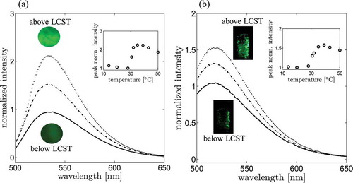
Fluorescence quantum yields of Nitrobenzofurazan-based dyes are very low in water (1–2%). However, interaction with the polymer moiety above LCST can substantially increase their fluorescence, due to the reduction of micro-environmental polarity experienced by the fluorescent units [32]. The increased fluorescence of the polymer is related to the thermodynamic transition at LCST [32]. Above 32 °C, PNIPAAm-based polymers present a dramatic reduction of the solubility of the chains in water, which is followed by a collapse of the individual chains and transition from an open coil to a closed globular conformation [47]. During this transition, the micro-environmental polarity in the vicinity of the PNIPAAm chains experiences a substantial decrease, which, in turn, results in the increased fluorescence quantum yield of the NBD-AE units. The increase in the fluorescence emission is observed macroscopically in the polymer when the temperature rises above LCST. However, coalescence and aggregation of chain globules is responsible for the progressive reduction of the polymer fluorescence at higher temperatures (above 40 °C). Thermodynamic transition above LCST is reversible, and the open coil conformation of the chains is recovered when temperature is lowered below 32 °C [47]. Due to the increased polarity in the vicinity of the chains, fluorescence intensity of the polymer returns to its initial value after transition below LCST [32].

Similarly, Figure 4(b) displays the fluorescence emission spectra of the microparticles at 28, 31, and 35 °C. Spectra are normalized with respect to the polymer emission at 20 °C. In the inset, the value of the peak of the normalized fluorescence spectra is displayed as a function of the solution temperature in the range 14 to 50 °C. Notably, the sharp increase in the fluorescence emission above LCST is more spread out for the particles as compared to the polymer. In addition, we observe that the position of the fluorescence emission peak (518–520 nm) is blue-shifted of approximately 15 nm with respect to the polymer emission. We attribute this shift to the interaction of the fluorescent polymer with the PDMS matrix and the surfactants used during the preparation of the particles.

The morphology of the microparticles is displayed in Figure 5. More specifically, Figure 5(a) displays a fluorescence micrograph recorded using the optical microscope and Figure 5(b) displays a scanning electron micrograph. The images clarify the particles’ morphology, where the fluorescent polymer solution is contained in small enclosures incorporated within the transparent PDMS matrix. This composite structure allows for the detection of the fluorescence emission of the polymer, while preventing large-scale coalescence of the polymer above LCST. The rapid coalescence of PNIPAAm polymers inhibits the use of pure PNIPAAm hydrogel particles as temperature sensors in PIV applications.

Figure 5. (a) Optical micrograph of the fluorescent particle tracers. (b) Scanning electron micrograph of the particles. (c) Particle diameter distribution obtained from SEM images.

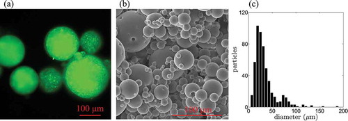
Figure 5(c) displays the size distribution of the particles obtained through the analysis of a set of scanning electron micrographs recorded at magnifications ranging from 100 to 400X. Size measurements are conducted using MATLAB on a sample of 500 particles randomly selected from the micrographs. Particles diameters are in the range 20–200 µm, with a mean diameter of 34 µm and a standard deviation of 23 µm.

3.2. PIV experiments

The particle tracers are used to measure the flow velocity in the cross flow of the cylinder using the apparatus introduced in Section 2. Flow around a bluff body is characterized by the presence of a wake region behind the body [48,49]. In specific flow regimes, the flow past the body is characterized by the release of vortices from the solid surface into the wake, such as the Karman vortex street in the wake of a cylinder [50,51].

The flow regime in the wake of the cylinder is governed by the Reynolds number [52,53]⁴, which is a non-dimensional parameter relating the magnitude of inertial to viscous forces in the fluid [53]. For the flow past a cylinder, the Reynolds number is defined as

(2)

For Re ≲ 5, the wake is laminar and the flow is attached to the cylinder surface. As Re increases, the generation of a small recirculation region in the near wake behind the body is observed. For Re ≳ 40, the wake is characterized by the shedding of vortices from the surface of the cylinder into the flow. Up to Re ≈ 150, these vortices are periodically shed in the flow and within the interval 150 ≲ Re ≲ 300, the onset of turbulent structures in the laminar flow may be observed. The vortex shedding partially loses its periodicity due to the transition.

For 300 ≲ Re ≲ 10⁴, the vortices are irregular due to the onset of turbulence in the wake; however, a predominant shedding frequency may be determined [52]. Above Re ≈ 10⁵, the wake is fully turbulent [53]. For the experiments presented in this work, Re = 291 for V₀ = 15.3 mm/s and Re = 583 for V₀ = 30.7 mm/s. In this range, the wake should be characterized by the nearly periodic release of vortices in the wake.

Periodicity of the vortex shedding phenomenon is investigated through numerical simulation of the wake past the cylinder. Numerical simulations are conducted to account for the effects of the non-uniform upstream velocity distribution and the cylinder blockage on flow physics and shedding period. The simulations are performed by using the flow velocity displayed in Figure 3(c), red line, as the initial velocity at the inlet of the channel. Details on the simulation are included in the Appendix. From the analysis, we obtain a shedding period of 3.3 s for V₀ = 15.3 mm/s and a shedding period of 1.8 s for V₀ = 30.7 mm/s⁵.

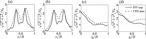
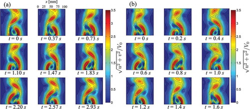
Figure 6(a,b) display the instantaneous velocity for V₀ = 15.3 mm/s and 30.7 mm/s in nine consecutive instants over one shedding period. In accordance to Figure 3, the cylinder is located outside the field of view in the bottom center of the image with respect to the ROI. The instantaneous velocity over one period is computed as the mean of the instantaneous velocity over three periods for V₀ = 15.3 mm/s (12 seconds) and 30.7 mm/s (5.4 seconds). Figure 7(a,b) display the average flow velocity at y/B = D/B for V₀ = 15.3 mm/s and 30.7 mm/s, respectively. Figure 7(c,d) illustrate the average flow velocity at x/B = 0.5-D/B for V₀ = 15.3 mm/s and 30.7 mm/s, respectively. The average velocity is computed as the sum of the velocities in the frames over one period divided by the number of frames in the period.

Figure 6. (a) Flow velocities measured during the PIV experiment at nine successive time instants t over one shedding period for V₀ = 15.3 mm/s. (b) Flow velocities measured during the PIV experiment at nine successive time instants t over one shedding period for V₀ = 30.7 mm/s.

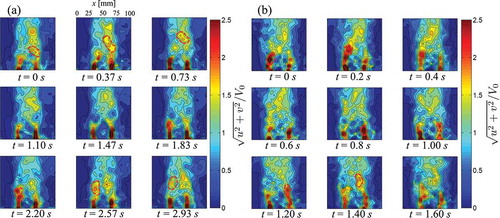
Figure 7. (a) Average flow velocity over one period at y/B = D/B for V₀ = 15.3 mm/s. (b) Average flow velocity over one period at y/B = D/B for V₀ = 30.7 mm/s. (c) Average flow velocity over one period at x/B = 0.5 – D/B for V₀ = 15.3 mm/s. (d) Average flow velocity over one period at x/B = 0.5 – D/B for V₀ = 30.7 mm/s. Solid lines are experimental PIV velocities and dashed-dotted lines are numerical results obtained using the computer simulation described in the Appendix.

By analyzing the experimental flow velocity in the near wake close to the cylinder in Figure 6 and Figure 7(a,b), we detect the presence of two high velocity regions, located on the sides of the cylinder. The maximum experimental velocity measured in these regions is 54 mm/s for V₀ = 15.3 mm/s and 107 mm/s for V₀ = 30.7 mm/s. In the center of the wake behind the cylinder, we observe the presence of a low velocity recirculation region, with velocities on the order of 8 mm/s for V₀ = 15.3 mm/s and of 20 mm/s for V₀ = 30.7 mm/s.

High velocities in the near wake are related to the blockage effect [54], which causes an acceleration of the flow in the channel and the onset of the recirculation region behind the cylinder. From the analysis of the average velocities in Figure 7(a,b), we find a good agreement between the experimental PIV data and numerical model in the Appendix. In particular, an excellent agreement is observed for the fastest flow (V₀ = 30.7 mm/s). For V₀ = 15.3 mm/s, the flow velocity matches well in the central section of the channel, while we note that the experimental velocity on the sides is lower than the velocity predicted from the numerical analysis.

High velocity regions are also found in the wake far from the cylinder. These regions are outlined with red dashed lines in Figure 6. We relate the presence of these features to the generation of vorticity on the surface of the cylinder and vortex shedding in the wake. By comparing the experimental flow velocities with numerical findings displayed in Figure A1 in the Appendix, we note that vortex structures predicted by the simulation are only partially reconstructed from PIV. In addition, from the analysis of the average velocities in Figure 7(c,d), we find that experimental velocity in the wake decreases faster than numerical predictions.

As the wake develops and the velocity decreases, the initial shape of the high velocity regions is rapidly lost, and the periodicity of the vortex shedding can be only partially inferred from the experimental flow velocity. This reduction of the flow velocity and loss of the temporal and geometrical periodicity is attributed to three-dimensional effects generated by the uneven velocity distribution within the depth of the channel, as discussed in Section 2. In addition, the initial onset of turbulent structures is expected in these flow regimes (Re ≥ 300) with a consequent disruption of the periodicity of the flow as the wake develops [52].

Fluorescence emission of the tracers is used for detection of high temperature regions in the flow, following the image-based procedure described in Section 2. Figure 8(a,b) display the results for the particle count procedure for V₀ = 15.3 mm/s and 30.7 mm/s, respectively. The particle count is performed by averaging a total of 4000 images measured during four independent 20 s acquisition intervals. The plots in Figure 8(a,b) display the number of interrogation regions used in the fluorescence analysis as a function of the number of particles per second detected in each interrogation region corrected by the effective seeding density (for = 10, we found =2.44, =4.1 for V₀ = 15.3 mm/s and =1.92, =5.2 for V₀ = 30.7 mm/s). According to experimental observations, the number of particles detected is higher when the temperature on the surface of the cylinder is set to 60 °C. The higher temperature in the wake enhances particle fluorescence and, in turn, increases the number of particles detected by the camera-filter system.

Figure 8. (a) Number of interrogation regions (10 × 10 pixels) is reported as a function of the number of particles per second detected in each region for V₀ = 15.3 mm/s, corrected by the factor κ = 2.44. (b) Number of interrogation regions (10 × 10 pixels) is reported as a function of the number of particles per second detected in each region for V₀ = 30.7 mm/s, corrected by the factor κ = 1.92. Red is the particle count when the cylinder is at 60°C, and black refers to the experiment in which the cylinder is kept at room temperature. In the insets, spatial distribution of the corrected particles/second value in the ROI, obtained by subtracting the particle distribution measured at room temperature from the particle distribution measured at 60 °C. White lines are contour lines of the time averaged velocity field (8 seconds) estimated using PIV data. The position of the cylinder and the flow direction are indicated below the insets.

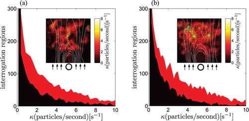
The spatial distribution of the particles is displayed in the insets of Figure 8(a,b). These temperature maps are obtained by subtracting the particle distribution obtained at room temperature from the particle distribution obtained at 60 °C⁶. By analyzing the mean flow streamlines superimposed to the temperature map in the insets, we find a high concentration of the particles in the central region of the flow, starting approximately 1–1.5 D downstream from the cylinder, see Figure 6. The presence of this high temperature region may be related to the three-dimensional effects noted in the PIV analysis. The progressive velocity decrease and the disruption of the vortex structures may be associated to mixing of the main flow with secondary flows in lower sections of the tank, which are characterized by a higher temperature due to lower flow velocities.

However, this observation may also be related to a slightly delayed time response of the particles after transition through the high temperature region close to the cylinder. While relaxation times for the coil-to-globule transition of PNIPAAm polymers are on the order of 10–100 ms [47] and the expected time response of the particle is on the order of 10–50 ms⁷, we may not exclude the possibility of slower responses for the particles due to the encapsulation of the fluorescent polymer in the PDMS matrix. In addition, particles’ detection may also be influenced by variations in the intensity of the laser beam within the ROI, which would partially explain the reduced particle count on the top and bottom boundaries.

4. Conclusions

In this paper, we put forward a methodology for the design of active tracers for temperature sensing in water, and we discussed in detail their potential implementation in PIV. The particles were developed using state-of-the-art, advanced polymer sensors with high temperature sensitivity in water based on Nitrobenzofurazan functionalized PNIPAAm. Different from previous studies, the particles were specifically designed to be employed without any modification to classical PIV systems, whereby the only required upgrade would be the use of a bandpass filter to isolate the particle fluorescence from the background scattered radiation. In addition, the choice of a hydrophilic and biocompatible polymer, such as PNIPAAm, may promote the application of these sensors in biology and environmental engineering.

The particles were prepared using a water-in-oil-in-water double emulsion technique, whereby thermosensitive NBD-AE-co-PNIPAAm polymers were incorporated within an optically transparent PDMS matrix. In line with results reported in the literature [32], we observed a more than twofold increase of polymer fluorescence upon transition above 32 °C. A similar behavior was found after encapsulation of the fluorescent polymer solution in the PDMS, with particles fluorescence increasing of approximately one and a half times when water temperature raised above 32 °C.

We demonstrated the application of these sensors in PIV by investigating the wake of a heated cylinder in water. Dedicated PIV experiments were conducted to reconstruct the flow velocity and identify high temperature regions in the wake. Two separate experimental conditions were explored with nominal upstream flow velocities of 15.3 mm/s and 30.7 mm/s. The flow analysis allowed for the detection of high velocity regions on the sides of the cylinder, the recirculation region in the wake behind the cylinder, and the shedding of vortices from the cylinder surface into the wake.

With respect to thermal analysis, for both values of the upstream flow velocity, we performed two experiments. In the first experiment, the cylinder was kept at room temperature, and in the second, we set the temperature on its surface to 60 °C. The fluorescence emission of the particles was quantified via a particle count procedure, whereby a bandpass filter was used to isolate the NBD-AE-co-PNIPAAm fluorescence from laser scattering. Using this technique, more particles were detected in the flow when the temperature of the cylinder was set to 60 °C, thereby demonstrating the ability of the particles to detect variable temperature fields through a measurable increase in their fluorescence. However, accurate spatial reconstruction of the high temperature regions in the wake of the cylinder was limited in this experiment.

Future studies might focus on different aspects of the PIV system presented in this work. First, the optical response of the particles could be improved by exploring different classes of fluorescent dyes with stronger emission [31,55], as well as photonic crystals [24,56] and plasmonic systems [57]. Another important area of improvement could be the modulation of the particles’ temperature response. Particles that respond to different temperature ranges could be prepared by employing copolymers with different LCST than NIPAAm [56,58]. We envision the simultaneous use of particles embedding different dye systems (different emission wavelengths/colors) and variable temperature responses, towards a full resolution of wide temperature ranges in terms of relative color gradients. Finally, the optimization of the image acquisition system and the adoption of more sophisticated pulsed lasers may be desired to improve spatial fluorescence measurements in complex flow regimes, such as the flow in the wake of a rigid cylinder discussed in this work.

Acknowledgments

The authors want to thank Dr. Avi Ulman and the Institute for Engineered Interfaces (IEI) at the New York University Tandon School of Engineering for granting access to the laboratories.

Disclosure statement

No potential conflict of interest was reported by the authors.

Additional information

Funding

This research was conducted with the support of the National Science Foundation through Grant No. CBET-1332204. The authors also acknowledge support from the Office of Naval Research through Grant No. N00014-10-1-0988, which has allowed the acquisition of equipment used in this study. This work was supported by the Division of Chemical, Bioengineering, Environmental, and Transport Systems [1332204].

Notes

1. Experimental observations show that the size of the particles can be modulated by varying the amount of SDS in the water emulsion.

2. The cylinder blockage factor is D/B = 0.19. This is considered a large blockage, and as such the fluid flow around the cylinder is expected to be significantly influenced by the presence of the walls.

3. St below 0.1 is generally the rule of thumb in the design of PIV experiments. The larger particles are expected to perform less well in flows with short time scales, such as turbulence.

4. The possibility of inferring the flow physics using only the Reynolds number should be considered strictly valid only for minimal blockage and deep channels, where boundary and three-dimensional effects are secondary.

5. The period of vortex shedding obtained using the simulation is shorter than the period estimated using an empirical relation [51], for vortex shedding from a cylinder in a uniform axial flow. Using this relation, we would obtain a shedding period of 6.32 and 3.03 seconds for V₀ = 15.3 mm/s and V₀ = 30.7 mm/s, respectively.

6. As discussed in Section 2, temperature in the tanks is not allowed to exceed 28 °C during the experiments.

7. The time response of a particle can be roughly estimated through the solution of the classical heat transfer equation for a hollow sphere as , with being the thermal resistance of the PDMS shell. In this equation, , are the external and internal radii of the particle, = 0.15 W/(m K) is the thermal conductivity of PDMS, = 4.18 kJ/(kg K) is the heat capacity of water, =1000 kg/m3 is the density of water, and and are the final and initial temperature differences between the solution contained in the particle and the external flow. Using this relation with = 80 µm, = 60 µm, = 20 °C, and = 0.1 °C, we find = 44 ms.

Appendix

Here, we analyze the flow field in the wake of the cylinder using the software COMSOL. The two-dimensional finite element simulation is conducted to: i) predict the vortex shedding frequency and ii) investigate the flow physics in the wake of the cylinder. The fluid domain has dimensions 100 × 500 mm². The cylinder is positioned at the center of the channel 150 mm from the inlet. The fluid is modeled as a viscous, incompressible, Newtonian fluid using the preset ‘water’ material function in COMSOL. A ‘free triangular’ mesh is used to discretize the fluid domain with 5910 elements with a maximum element size of 5 mm on the contour of the domain and a minimum element size of 0.008 mm on the boundary of the cylinder. The solution is obtained using the ‘time-dependent’ solver in COMSOL with a time step of 0.0005 s for V₀ = 15.3 mm/s and 0.0001 s for V₀ = 30.7 mm/s. The Courant-Friedrichs-Lewy number for the simulation is 0.96 for V₀ = 15.3 mm/s and 0.39 for V₀ = 30.7 mm/s [59].

Figure A1. (a) Flow velocities at nine successive time instants t over a time period for V0 = 15.3 mm/s. (b) Flow velocities at nine successive time instants t over a time period for V0 = 30.7 mm/s.

The following boundary conditions are imposed on the fluid domain: i) a no-slip boundary condition on the side walls of the tank and on the cylinder to impose zero velocity; ii) a zero pressure and no viscous stress condition at the outlet of the channel; and iii) a velocity equivalent to the experimental average velocity at the inlet of the channel. The velocity profile at the inlet of the channel is obtained by fitting the average velocity displayed in Figure 3 with a Fourier series

For the average velocity in Figure 3, we find for N = 3: A₁ = 2.06, a₂ = 0.10, a₃ = 0.79, b₁ = 3.54, b₂ = 18.62, b₃ = 10.94, c₁ = −0.26, c₂ = −1.64, and c₃ = −4.08.

Figure A1(a,b) show the flow velocity in the 100 × 100 mm² region in the wake of the cylinder for V₀ = 15.3 mm/s and 30.7 mm/s, respectively. This region matches the ROI investigated in the PIV experiment in Figure 6. We obtain a period of vortex shedding of 3.3 s for V₀ = 15.3 mm/s and 1.8 s for V₀ = 30.7 mm/s. The period is determined by matching the velocities at successive time steps until two equivalent instantaneous flow velocities are found. Matching of the frames is performed after the wake has fully developed in the simulation, a condition that is obtained after 40 s for V₀ = 15.3 mm/s and after 11 s for V₀ = 30.7 mm/s. The vortex shedding phenomenon is clearly reconstructed by the computer simulation. High velocity regions are related to shedding in the wake of vorticity generated on the surface of the cylinder [53,54].

References

- R.J. Adrian and J. Westerweel, Particle Image Velocimetry, Cambridge University Press, Cambridge, 2011.
- M. Raffel, C.E. Willert, S. Wereley, and J. Kompenhans, Particle Image Velocimetry: A Practical Guide, Springer, New York, 2013.
- A. Cotroni, F. Di Felice, G.P. Romano, and M. Elefante, Investigation of the near wake of a propeller using particle image velocimetry, Exp. Fluids 29 (2000), pp. 227–236. doi:10.1007/s003480070025
- E.W.M. Roosenboom, A. Heider, and A. Schröder, Investigation of the propeller slipstream with particle image velocimetry, J. Aircr. 46 (2009), pp. 442–449. doi:10.2514/1.33917
- U. Dierksheide, P. Meyer, T. Hovestadt, and W. Hentschel, Endoscopic 2D particle image velocimetry (PIV) flow field measurements in IC engines, Exp. Fluids. 33 (2002), pp. 794–800. doi:10.1007/s00348-002-0499-3
- D.L. Reuss, R.J. Adrian, C.C. Landreth, D.T. French, and T.D. Fansler, Instantaneous planar measurements of velocity and large-scale vorticity and strain rate in an engine using particle-image velocimetry. SAE Technical Paper, 1989.
- X. Cao, J. Liu, N. Jiang, and Q. Chen, Particle image velocimetry measurement of indoor airflow field: A review of the technologies and applications, Energy Build. 69 (2014), pp. 367–380. doi:10.1016/j.enbuild.2013.11.012
- J. Hong, M. Toloui, L.P. Chamorro, M. Guala, K. Howard, S. Riley, J. Tucker, and F. Sotiropoulos, Natural snowfall reveals large-scale flow structures in the wake of a 2.5-MW wind turbine, Nat. Commun. 24 (2014), pp. 1–9.
- F. Tauro, M. Porfiri, and S. Grimaldi, Surface flow measurements from drones, J. Hydrology. 540 (2016), pp. 240–245. doi:10.1016/j.jhydrol.2016.06.012
- M. Ferrari, R. Bashir, and S.T. Wereley, BioMEMS and Biomedical Nanotechnology. Volume IV: Biomoleculars Sensing, Processing and Analysis, Springer, New York, 2007.
- S.D. Peterson and M.W. Plesniak, The influence of inlet velocity profile and secondary flow on pulsatile flow in a model artery with stenosis, J. Fluid Mech. 616 (2008), pp. 263–301. doi:10.1017/S0022112008003625
- S.G. Chopski, O.M. Rangus, C.S. Fox, W.B. Moskowitz, and A.L. Throckmorton, Stereo-particle image velocimetry measurements of a patient-specific fontan physiology utilizing novel pressure augmentation stents, Artif. Organs. 39 (2015), pp. 228–236. doi:10.1111/aor.2015.39.issue-3
- B. Peterson, E. Baum, B. Bohm, V. Sick, and A. Dreizler, High-speed PIV and LIF imaging of temperature stratification in an internal combustion engine. Proceedings of the Combustion Institute, 2013. 34: p. 3653–3660.
- P. Chamarthy, S.V. Garimella, and S.T. Wereley, Non-intrusive temperature measurement using microscale visualization techniques, Exp. Fluids 47 (2009), pp. 159–170. doi:10.1007/s00348-009-0646-1
- J. Massing, D. Kaden, C.J. Kahler, and C. Cierpka, Luminescent two-color tracer particles for simultaneous velocity and temperature measurements in microfluidics, Meas. Sci. Technol. 27 (11) (2016), pp. 115301. doi:10.1088/0957-0233/27/11/115301
- C. Abram, B. Fond, A.L. Heyes, and F. Beyrau, High-speed planar thermometry and velocimetry using thermographic phosphor particles, Appl. Phys. B-Lasers Opt. 111 (2) (2013), pp. 155–160. doi:10.1007/s00340-013-5411-8
- C. Abram, M. Pougin, and F. Beyrau, Temperature field measurements in liquids using {ZnO} thermographic phosphor tracer particles, Exp. Fluids. 57 (2016), pp. 115. doi:10.1007/s00348-016-2200-2
- J. Sakakibara and R.J. Adrian, Measurement of temperature field of a Rayleigh-Benard convection using two-color laser-induced fluorescence, Exp. Fluids. 37 (3) (2004), pp. 331–340. doi:10.1007/s00348-004-0821-3
- A. Charogiannis, I. Zadrazil, and C.N. Markides, Thermographic particle velocimetry TPV for simultaneous interfacial temperature and velocity measurements, Int. J. Heat Mass Transf. 97 (2016), pp. 589–595. doi:10.1016/j.ijheatmasstransfer.2016.02.050
- C.R. Smith, D.R. Sabatino, and T.J. Praisner, Temperature sensing with thermochromic liquid crystals, Exp. Fluids. 30 (2001), pp. 190–201. doi:10.1007/s003480000154
- H. Li, C. Xing, and M.J. Braun, Natural convection in a bottom-heated top-cooled cubic cavity with a baffle at the median height: Experiment and model validation, Heat Mass. Transfer. 43 (2007), pp. 895–905. doi:10.1007/s00231-006-0178-7
- E. Spinosa and S. Zhong, Application of Liquid Crystal Thermography for the investigation of the near-wall coherent structures in a turbulent boundary layer, Sens. Actuators, A. 233 (2015), pp. 207–216. doi:10.1016/j.sna.2015.05.026
- D. Dabiri, Digital particle image thermometry/velocimetry: A review, Exp. Fluids. 46 (2) (2009), pp. 191–241. doi:10.1007/s00348-008-0590-5
- A. Seeboth, D. Lotzsch, R. Ruhmann, and O. Muehling, Thermochromic polymers-function by design, Chem. Rev. 114 (5) (2014), pp. 3037–3068. doi:10.1021/cr400462e
- M. Carlotti, G. Gullo, A. Battisti, F. Martini, S. Borsacchi, M. Geppi, G. Ruggeri, and A. Pucci, Thermochromic polyethylene films doped with perylene chromophores: Experimental evidence and methods for characterization of their phase behaviour, Polym. Chem. 6 (2015), pp. 4003–4012. doi:10.1039/C5PY00486A
- A. Seeboth, D. Lotzsch, and R. Ruhmann, First example of a non-toxic thermochromic polymer material based on a novel mechanism, J. Mater. Chem. C. 1 (2013), pp. 2811–2816. doi:10.1039/c3tc30094c
- Y. Iijima and H. Sakaue, Platinum porphyrin and luminescent polymer for two-color pressure- and temperature-sensing probes, Sens. Actuators, A. 184 (2012), pp. 128–133. doi:10.1016/j.sna.2012.06.033
- M. Culebras, A.M. Lopez, C.M. Gomez, and A. Cantarero, Thermal sensor based on a polymer nanofilm, Sens. Actuators, A. 239 (2016), pp. 161–165. doi:10.1016/j.sna.2016.01.010
- C.-L. Lee, Y.-W. You, J.-H. Dai, J.-M. Hsu, and J.-S. Horng, Hygroscopic polymer microcavity fiber Fizeau interferometer incorporating a fiber Bragg grating for simultaneously sensing humidity and temperature, Sens. Actuators, B. 222 (2016), pp. 339–346. doi:10.1016/j.snb.2015.08.086
- T. Ioppolo and M. Manzo, Dome-shaped whispering gallery mode laser for remote wall temperature sensing, Appl. Opt. 53 (2014), pp. 5065–5069. doi:10.1364/AO.53.005065
- M. Barbieri, F. Cellini, I. Cacciotti, S.D. Peterson, and M. Porfiri, In situ temperature sensing with fluorescent chitosan-coated PNIPAAm/alginate beads, J. Mater. Sci. 52 (2017), pp. 12506–12512. doi:10.1007/s10853-017-1345-6
- S. Uchiyama, Y. Matsumura, A.P. de Silva, and K. Iwai, Fluorescent molecular thermometers based on polymers showing temperature-induced phase transitions and labeled with polarity-responsive benzofurazans, Anal. Chem. 75 (21) (2003), pp. 5926–5935. doi:10.1021/ac0346914
- E. Yoshinari, H. Furukawa, and K. Horie, Fluorescence study on the mechanism of rapid shrinking of grafted poly(N-isopropylacrylamide) gels and semi-IPN gels, Polymer. 46 (18) (2005), pp. 7741–7748. doi:10.1016/j.polymer.2005.01.100
- Y. Shiraishi, R. Miyamoto, X. Zhang, and T. Hirai, Rhodamine-based fluorescent thermometer exhibiting selective emission enhancement at a specific temperature range, Org. Lett. 9 (20) (2007), pp. 3921–3924. doi:10.1021/ol701542m
- P. Kumari, M.K. Bera, S. Malik, and B.K. Kuila, Amphiphilic and thermoresponsive conjugated block copolymer with its solvent dependent optical and photoluminescence properties: Toward sensing applications, ACS Appl. Mater. Interfaces. 7 (23) (2015), pp. 12348–12354. doi:10.1021/am507266e
- Y. Shiraishi, R. Miyamoto, and T. Hirai, Rhodamine-conjugated acrylamide polymers exhibiting selective fluorescence enhancement at specific temperature ranges, J. Photochem. Photobiology A: Chem. 200 (2–3) (2008), pp. 432–437. doi:10.1016/j.jphotochem.2008.08.020
- X. Hu, Y. Li, T. Liu, G. Zhang, and S. Liu, Intracellular cascade FRET for temperature imaging of living cells with polymeric ratiometric fluorescent thermometers, ACS Appl. Mater. Interfaces. 7 (2015), pp. 15551–15560. doi:10.1021/acsami.5b04025
- T. Hayashi, N. Fukuda, S. Uchiyama, and N. Inada, A cell-permeable fluorescent polymeric thermometer for intracellular temperature mapping in mammalian cell lines, PLoS ONE. 10 (2) (2015), pp. 1–18. doi:10.1371/journal.pone.0117677
- K. Okabe, N. Inada, C. Gota, Y. Harada, T. Funatsu, and S. Uchiyama, Intracellular temperature mapping with a fluorescent polymeric thermometer and fluorescence lifetime imaging microscopy, Nat. Commun. 3 (2012), pp. 705. doi:10.1038/ncomms1714
- S. Freddi, L. Sironi, R. D’Antuono, D. Morone, A. Dona, E. Cabrini, L. D’Alfonso, M. Collini, P. Pallavicini, G. Baldi, D. Maggioni, and G. Chirico, A molecular thermometer for nanoparticles for optical hyperthermia, Nano Lett. 13 (5) (2013), pp. 2004–2010. doi:10.1021/nl400129v
- M. Onoda, S. Uchiyama, T. Santa, and K. Imai, A photoinduced electron-transfer reagent for peroxyacetic acid, 4-Ethylthioacetylamino-7- phenylsulfonyl-2,1,3-benzoxadiazole, based on the method for predicting the fluorescence quantum yields, Anal. Chem. 74 (16) (2002), pp. 4089–4096. doi:10.1021/ac0201225
- B.J. Sun, Y.A. Lin, and P.Y. Wu, Structure analysis of poly(N-isopropylacrylamide) using near-infrared spectroscopy and generalized two-dimensional correlation infrared spectroscopy, Appl. Spectrosc. 61 (7) (2007), pp. 765–771. doi:10.1366/000370207781393271
- W.-C. Tian and E. Finehout, Microfluidics for Biological Applications, Springer, New York, 2009.
- W. Thielicke and E.J. Stamhuis, PIVlab - Towards user-friendly, affordable and accurate digital particle image velocimetry in MATLAB, J. Open Res. Software. 2 (1) (2014), pp. e30. doi:10.5334/jors.bl
- P. Ramaprabhu and M.J. Andrews, Simultaneous measurements of velocity and density in buoyancy-driven mixing, Exp. Fluids. 34 (2003), pp. 98–106. doi:10.1007/s00348-002-0538-0
- A.N. Bashkatov and E.A. Genina Water refractive index in dependence on temperature and wavelength: A simple approximation, Proceedings Volume 5068, Saratov Fall Meeting 2002: Optical Technologies in Biophysics and Medicine IV. 2002.
- H. Inoue, S. Kuwahara, and K. Katayama, The whole process of phase transition and relaxation of poly(N-isopropylacrylamide) aqueous solution, Phys. Chem. Chem. Phys. 15 (11) (2013), pp. 3814–3819. doi:10.1039/c3cp43309a
- A.E. Perry, M.S. Chong, and T.T. Lim, The vortex-shedding process behind two-dimensional bluff bodies, J. Fluid Mech. 116 (1982), pp. 77–90. doi:10.1017/S0022112082000378
- A. De Rosis, G. Falcucci, S. Ubertini, and F. Ubertini, A coupled lattice Boltzmann-finite element approach for two-dimensional fluid–Structure interaction, Comput. Fluids. 86 (2013), pp. 558–568. doi:10.1016/j.compfluid.2013.08.004
- H. Oertel Jr, Wakes behind blunt bodies, Annu. Rev. Fluid Mech. 22 (1) (1990), pp. 539–562. doi:10.1146/annurev.fl.22.010190.002543
- G. Di Pasquale, S. Graziani, A. Pollicino, and S. Strazzeri, A vortex-shedding flowmeter based on IPMCs, Smart Mater. Struct. 25 (1) (2016), pp. 015011. doi:10.1088/0964-1726/25/1/015011
- A. Roshko, On the development of turbulent wakes from vortex streets, NACA Report 1191, 1953.
- R.D. Blevins, Flow-Induced Vibration, Van Nostrand Reinhold Co, New York, 1977.
- M. Sahin and R.G. Owens, A numerical investigation of wall effects up to high blockage ratios on two-dimensional flow past a confined circular cylinder, Phys. Fluids. 16 (2004), pp. 1305–1320. doi:10.1063/1.1668285
- C.D.S. Brites, P.P. Lima, N.J.O. Silva, A. Millan, V.S. Amaral, F. Palacio, and L.D. Carlos, Thermometry at the nanoscale, Nanoscale. 4 (2012), pp. 4799–4829. doi:10.1039/c2nr30663h
- H. Kye, Y.G. Koh, Y. Kim, S.G. Han, H. Lee, and W. Lee, Tunable temperature response of a thermochromic photonic gel sensor containing N-Isopropylacrylamide and 4-Acryloyilmorpholine, Sensors. 17 (6) (2017), pp. 1-10. doi: 10.3390/s17061398
- C.A.S. Burel, A. Alsayed, L. Malassis, C.B. Murray, B. Donnio, and R. Dreyfus, Plasmonic-based mechanochromic microcapsules as strain sensors, Small. 13 (39) (2017). doi:10.1002/smll.201701925
- F. Cellini, L. Block, J. Li, S. Khapli, S.D. Peterson, and M. Porfiri, Mechanochromic response of pyrene functionalized nanocomposite hydrogels, Sens. Actuators B. 234 (2016), pp. 510–520. doi:10.1016/j.snb.2016.04.149
- N.S. Bakhvalov, Courant-Friedrichs-Lewy condition, Encyclopedia Math. (2001).