Operational limits of a non-homogeneous dielectric elastomer transducer

ABSTRACT

Operation of a dielectric elastomer (DE) transducer is limited by the way it fails, and any other limits imposed by the user. For example, material rupture and dielectric breakdown are two examples of transducer failure, while tension loss is a user-imposed limit. Electromechanical instability may or may not result in transducer failure, but is often considered as a boundary to denote the onset of state transition. For a DE undergoing homogeneous deformation, constructing operational limits on work-conjugate state diagrams are rather straight-forward. However, for DE subjected to non-homogeneous deformation, the process is more complex. We present a method to plot the operational boundaries of a DE subject to non-homogeneous deformation, known commonly as the Universal Muscle Actuator or the loudspeaker configuration. Our analysis show that tension loss need not be imposed as a hard operational limit, and that there is further operational space for the transducer, post tension loss. By plotting the operational limits on work-conjugate planes, we determine an optimal inner-to-outer ring ratio and the required pre-stretches that maximize energy conversion.

KEYWORDS:

• Dielectric elastomer
• non-homogeneous
• operational limits
• loudspeaker configuration

Introduction

Dielectric elastomers (DE) convert mechanical energy and electrical energy interchangeably [1,2]. A DE consists of an elastomer membrane sandwiched between compliant electrodes. When a voltage is applied across the electrodes, the polymer thins down and expands in area due to electrostatic charges [3]. The pressure that arises due applied voltage is called Maxwell pressure [2,4]; the DE operates as an actuator. When a low voltage charge is placed on a stretched elastomer, the subsequent mechanical contraction against Maxwell pressure increases the potential (voltage) of the charge, thereby amplifying the electrical energy. Many DE configurations were proposed and studied. Some examples include equal-biaxial configuration [5], flat-clamped configuration [6], stacked configuration [7], tubular configuration [8], loudspeaker configuration [9] and parallelogram configuration [10].

Some of the configurations deform in a homogeneous manner, while others are non-homogeneous. For cases of homogeneous deformation, the governing equations and operational boundaries can be expressed as algebraic equations. For instance, equal-biaxial and flat-clamped configurations may be approximated to be homogeneous. Operational limits may be determined from the algebraic equations for such cases, facilitating plotting of work-conjugate state diagrams [10–13]. Such state diagrams prescribe the allowable regions of operation, which will aid in the design of operational cycles. However, many practical configurations of DE are subjected to non-homogeneous deformation. The general equations to model non-homogeneous configurations were presented in a previous work [14] but not specialized. We specialize such non-homogeneous formulations for a widely-used Universal Muscle Actuator [15], also known as the loudspeaker configuration, and use it to study the deformation characteristics, practical operational limits and performance limits for such a configuration.

The loudspeaker configuration is popular due to ease of fabrication with fully covered edges, and it is easy to produce multiple layers of such a configuration. As such, the loudspeaker configuration is extensively used as actuators [16–18] and energy harvesters [19–21]. The analytical models of loudspeaker DE were presented previously [9,19,22]. A simplified method of plotting operational boundaries of a loudspeaker configuration DE in voltage-force plane was also done based on the analytical model [23]. However, these studies cover only part of the operational regime of a loudspeaker configuration, and missed other possible states, especially in the high voltage and high stretch region. For example, at moderate to high electric field, a DE membrane loses tension, and buckles under a very small compressive stress leading to pull-in instability [6]. The above mentioned analytical models do not capture this. Our model predicts the stretch states of the DE post tension loss.

To cover all operational possibilities of a loudspeaker configuration, we adopt the approach of plotting operational limits on a work-conjugate state diagram. A dielectric elastomer fails [11] by mechanical rupture and electric breakdown. These shall form the first two hard operational limits of our analysis. Electromechanical transition leading to instability (EMI) is also commonly cited as an operational limit, as it may lead to dielectric breakdown. EMI is the positive feedback that takes place in a DE, where a thinning DE increases electric field, thereby inducing further thinning. Such an instability causes the DE to transit from a thick to a thin state of deformation. Our analysis will reveal that EMI does not take place in a DE in loudspeaker-type configuration. Tension loss may take place in both the hoop and axial directions. Our analysis will show that tension loss in the hoop direction simply indicates a transition from a flat to wrinkled deformation. A DE may therefore continue its operation even if there is tension loss [6]. The electrical breakdown and rupture limits are applied to the post tension loss states of the DE transducer to predict the operational limits. There are other instabilities identified for a dielectric elastomer transducer, like Rayleigh-Plateau instability [24] that arises due to the surface tension of the elastomer and snap-through instability experienced by an inflated diaphragm configuration of DE [25]. These instabilities maybe also analysed in a similar fashion to the post tension loss analysis, but are out of the scope of this paper. We plot these limiting conditions on work-conjugate state diagrams, to be used to compute the maximum possible energy for a loudspeaker-type configuration. The difference between a homogeneous and non-homogeneous deformation is that, for the latter, failure may occur locally. We further use the work-conjugate state diagrams the of loudspeaker configuration to locate optimal inner-to-outer ring ratios and equal biaxial pre-stretches that maximize energy conversion.

Analytical modelling and simulation

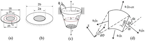
We begin by considering the geometry of a loudspeaker-type configuration, as shown in Figure 1. Force equilibrium requires that, and , where subscripts ‘r’ and ‘z’ refers to the radial and the axial directions, respectively. ‘’ denotes force. Applying force equilibrium in the ‘z’ direction, we have, from Figure 1d,

(1a)

Figure 1. Reference state (a) where the elastomer is unstretched and uncharged. A is the inner radius of the unstretched elastomer and B is the outer radius. Red circle denotes points at an arbitrary radius R. H is the initial thickness. Elastomer in (a) is biaxially prestretched and clamped at the outer and inner annulus (b). Inner and outer radius is constrained to a and b. The elastomer is then coated with complaint electrodes on both sides. Mechanical load F is applied in out of plane direction and a voltage of ϕ is applied as shown in (c). A section of (c) is enlarged in (d). Direction 1 is along the surface of Loudspeaker DEG towards the centre. Direction 2 is the hoops direction. s₁ and s₂ are the nominal stresses in 1 and 2 directions. λ₁ and λ₂ are stretches in 1 and 2 directions. θ is the angle the section makes with the horizontal plane. r and z are the coordinates of the deformed shape.

Integrating and simplifying (1a) gives,

(1b)

Applying force equilibrium in the ‘r’ direction (Figure 1d), Taylor expansion gives,

(2a)

Integrating and simplifying (2a) gives,

(2b)

Combining (1b) and (2b) we get,

(3)

Geometry in the radial direction gives (Figure 1d),

(4)

In the hoop direction, we have: (red line in Figure 1a and Figure 1c), hence,

(5)

Finally, geometry in the ‘z’ direction gives (Figure 1d),

(6)

A dielectric elastomer is deformed by both mechanical force and electric field. Hence, the energy density of a DE is written as . Where and are mechanical stretches and is the nominal electric displacement. From first-order variation of the Helmholtz free energy density, nominal stresses and are (Suo, 2010),

and .

We use the mechanical strain energy density given by Gent (Gent, 1996), and assume a linear dielectric, hence we have,

Where, . is the small strain shear modulus, is related to the theoretical material stretch limit and is the permittivity of the elastomer.

The explicit expressions for the nominal stresses are therefore,

(7a)

(7b)

From capacitance relationship of a linear dielectric (non-linear behaviour like polarization saturation [26] experienced by dielectric elastomer are not considered in this analysis), we have,

(7c)

Substituting (7c) into (7a) and (7b), we have,

(7d)

(7e)

Prescribing force F and voltage , applying boundary conditions r(A) = a, r(B) = b, we use (1b), (3), (4), (5), (7d) and (7e), and the shooting method to solve for . a is the radius of the inner ring and b is the radius of the outer ring. From these boundary values, the stretches and stresses are then solved by geometrically marching along the radial direction from A to B. z(R) is then solved from (6) and z(B) = 0.

Since the deformation is inhomogeneous, it follows that the capacitance is non-uniform we have,

(8a)

Where, . Integrating (8a) gives,

(8b)

And charge,

(9)

The total electric charge, may also be found by integrating with the initial (undeformed and uncharged) area.

Electric field,

(10a)

For an incompressible material, we have the final thickness,

(10b)

Substituting (10b) into (10a), we have,

(10c)

We non-dimensionalize all the physical quantities as follow,

, , , , , , , , ,

,

u is the out of plane displacement of the inner ring and represents energy.

The value of A to B ratio and prestretch, is chosen to be 0.5 and 2 respectively unless specified. VHB 4905 with [27] is used for the simulations. A sample of simulation result is given in Figure 2. The solution is compared with the existing literature [9] and the results are shown in Figure 3.

Figure 2. Sample of simulation result. Final deformed shape, λ₁ and λ₂, s₁ and s₂ and θ are plotted in (a), (b), (c) and (d) respectively. The simulation result is for, F = 1 and ϕ = 0 (solid line), ϕ = 0.2 (dashed line). A:B = 0.5 and λ_p = 2.

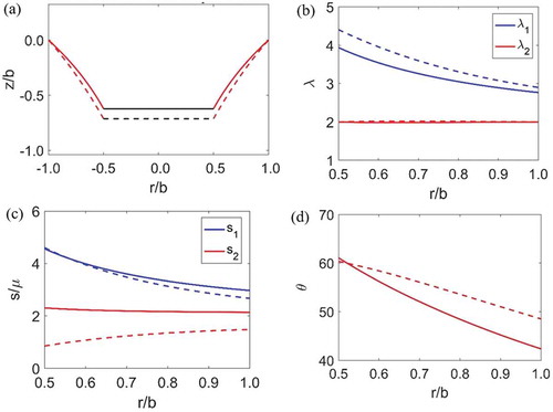
Figure 3. Force used is 0.5 (normalized with respect to b), prestretch used is 1.2 and A to B ratio is 0.25. Black, green, red and blue lines are for ϕ = 0, 0.15, 0.2 and 0.25 respectively. For (i) the J_lim used is, 120 and for (ii) it is 500. (iii) is re-created using the governing equations from [9]. In that paper, the material model used is Neo-Hookean. Hence the results for a larger value of J_lim (ii) matches with theirs.

Operation of DE bounded by limits

We use rupture, electric breakdown and loss of tension as operating limits. Electromechanical instability is not considered as an operating limit, which we shall explain in section on Electromechanical instability (EMI).

There is an inhomogeneous stretch distribution over the DE membrane. Failure will take place at localized points as opposed to an overall membrane failure for homogeneous deformation. We assume the membrane fails with failure of a point, and impose that as a limit.

Rupture

An elastomer ruptures when the applied stretch exceeds a maximum allowable stretch. For a membrane that is stretched in a biaxial manner, a combination of multi-axial stretch imposes the limit. For a material modelled by the Gent model, we impose a maximum value of J as the rupture limit, and term it . for VHB 4905 was taken to be the half of the . For uniaxial testing, we experimentally found that for VHB 4905, the material ruptures when J is nearly the half the value of (experimental results are given in the supplementary material).

Due to the inhomogeneous nature of deformation in a loudspeaker-type configuration, J will similarly be location-dependent. To plot this limit, we need to locate the position of maximum J, and then impose the rupture failure criterion is given by,

(11)

As the problem is highly nonlinear and there is no analytical solution, the approach is to find the voltage for a given force for which approaches . Then by substituting that force and voltage we can find the displacement and charge corresponding to it.

Electric breakdown

The electric breakdown strength for VHB 4905 used for this analysis is, 150MV/m [28]. This is equivalent to a value of 4.232 when non-dimensionalized using . The value of and used for this non dimensionalization are, F/m and 50 kPa respectively [27]. Electric breakdown strength is found to be dependent on the stretch [29]. But we shall ignore this variation in this analysis. For a dielectric membrane with inhomogeneous electric field, we assume that the membrane fails when the electric field of any point in the membrane exceeds the electric breakdown field [25]. We locate the position of maximum electric field and then impose the limit as,

(12a)

Equation (10c) in (12a) gives,

(12b)

The approach of estimating the state of the DE membrane for electric breakdown is similar as in the case of rupture.

Loss of tension (LT)

Loss of tension in loudspeaker configuration may take place in both the radial and/or the hoop direction(s). We shall consider both cases, as follows:

When tension loss takes place in the radial direction, we have:

Hence from equation (1e) gives, F = 0 and from equation (2c), . This implies that tension loss in the hoop direction will precede that in the radial direction, for a load-free DE (F = 0).

In a load-free condition, the loudspeaker will be planar, and ceases to take the shape of a loudspeaker geometry. Radial tension loss hence becomes a trivial condition for a DE in loudspeaker configuration. In our analysis, we ignore out-of-plane buckling due to Maxwell stress in a load-free configuration. Hence, we impose a minimum pre-stretch of 1.5 for the optimization in section, Optimizing maximum energy by geometry and pre-stretch.

When tension loss takes place in the hoop direction, we have:

is not uniform everywhere in the membrane (Figure 1c). This is because the stretch state of the loudspeaker membrane is non-uniform. Hence the more appropriate approach for checking the loss of tension is,

(13)

Similarly, with the previous approaches the method is to find the voltage for a given force at which the minimum value of across the loudspeaker membrane becomes zero. From that force and voltage, we can calculate the corresponding displacement and charge.

Electromechanical instability (EMI)

When voltage is increased, the elastomer reduces in thickness so that the positive feedback between a thinner elastomer and a higher true electric field may result in EMI [11].

Figure 4 shows a typical vs u plot for a loudspeaker configuration. u is the out-of-plane displacement of the inner circular plate. All responses are monotonic, implying the absence of unstable states corresponding to EMI, observed in homogeneous deformation. After tension loss, where there is a jump in stretch values [6], the membrane may or may not fail, which depends on the electric breakdown strength and the rupture limit. This is captured by the rupture and electric breakdown lines as shown in Figure 4. 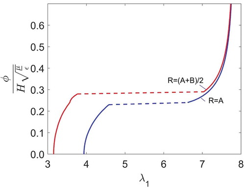The positive slope of the dashed lines in the vs u plot is because of the progression of wrinkles due to non-uniform stretch states on the membrane. Figure 5 explains this by taking two points, point A and the midway point between A and B for non-dimensionalized force of 1. We are assuming an elastomer with no defects. With the absence of nucleation sites, the elastomer can be super-charged [30]. Hence any instability will coincide with the point of lateral tension loss. For this reason, EMI is not considered in our analysis. For very large out-of-plane forces, beyond loss of tension the wrinkling in hoop direction shrinks the elastomer in the radial direction (Figure 4). This is indicated by a reduction of displacement.

Figure 4. Each black curve represents the state of loudspeaker DEG for a given force. An open circle represents the point of loss of tension. After loss of tension a new set of equations explained in section, ‘Post tension loss analysis’ are used. As the stretches are non-uniform, loss of tension and the instability in stretch occurs locally and progresses. This is represented by the dotted lines in the plot. The red curve represent rupture and the blue one represents electric breakdown. A:B = 0.5 and λ_p = 2.

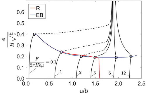
Figure 5. Voltage vs stretch at the inner ring and at the midway between inner and outer ring. Loss of tension and transition of stretches happens at different voltages. A:B = 0.5, λ_p = 2 and F = 1.

Minimum capacitance line

There is another boundary for a loudspeaker DE, when F = 0 and hence, the out-of-plane displacement is zero, corresponding to Figure 1c. We need to assign a line that corresponds to this minimum capacitance, as any out-of-plane deformation on the inner ring will increase the capacitance. We state this as the minimum capacitance line. The equation of this line is given by,

(14a)

From (8b) setting, , integrating we get,

(14b)

Post tension loss analysis

As electric field increases, part of the DE membrane loses tension. We model this by setting in equations (2) and (3). The consequence of this is that the membrane deforms as a truncated cone, as suggested by equation (3) in those regions. Due to inhomogeneous nature of this deformation, for regions where , equation (8) still holds and we use equation (1e) to estimate at those points.

For post tension loss analysis, the shooting method fails to provide a good initial estimate of . This is because of the inherent discontinuity at the boundaries where the membrane loses tension, and those that did not. Shooting method will fail to converge at a solution. For such instances, we use the bisection method to estimate

A similar method for a pure shear configuration was explained in a previous work [6]. The difference is that here is a function of R and (1e).

Figure 6 compares simulation results between simulations that analysed without mathematical consideration of post tension loss (dashed lines) and those with proper mathematical treatment of post tension loss. The latter shows much large deformation under the same loading conditions, with the ability to track the development of wrinkles (Figure 7).

Figure 6. Final deformed shape, λ₁ and λ₂, s₁ and s₂ and θ are plotted in (a), (b), (c) and (d) respectively. The simulation result is for, F = 1 and ϕ = 0.25. Solid lines represent the simulation result using the new set of equations beyond loss of tension and dashed lines are the results without considering them. A:B = 0.5 and λ_p = 2.

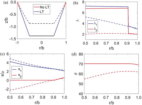
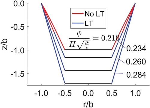
Figure 7. Progression of wrinkles. The simulation result is for, F = 1.5. At ϕ = 0.21, wrinkles appear near inner ring and at ϕ = 0.282, the entire membrane will be under loss of tension. A:B = 0.5 and λ_p = 2.

Experimental validation of the analytical model

The proposed model is validated experimentally. A loudspeaker configuration dielectric elastomer actuator is made of VHB 4905 (H = 0.5mm). The elastomer is pre-stretched equal biaxially with a pre-stretch, , the ring ratio (A:B) used is, 0.5 and the outer radius b is 5cm. We used carbon grease as the compliant electrodes. A constant load is added so that the out of plane displacement at 0V is 0.5 times of b. For the analytical plots of the experimental verification we used the average values of, and from Table 1 (Gent model curve fit of experimental data) in the supplementary materials. The value of permittivity used is F/m.

Table 1. Summary of tensile test data. is found nearly half of . The average value of from experiments is found to be 144.9. But for our analysis, we will still use the value of 120 from literature.

No.	(KPa)
1	26.2	129.6	8.2	64.2	0.49
2	26.2	142.0	8.8	74.8	0.52
3	26.2	148.9	8.8	74.7	0.50
4	24.9	142.4	8.8	74.2	0.52
5	26.2	141.6	8.7	72.5	0.51
6	25.3	145.5	9.0	78.3	0.54
7	28.4	140.3	8.6	70.8	0.50
8	25.5	142.9	8.5	70.1	0.49
9	21.2	153.4	8.9	76.5	0.50
10	24.2	162.3	9.0	78.4	0.48
Average	25.4	144.9	8.7	73.8	0.51

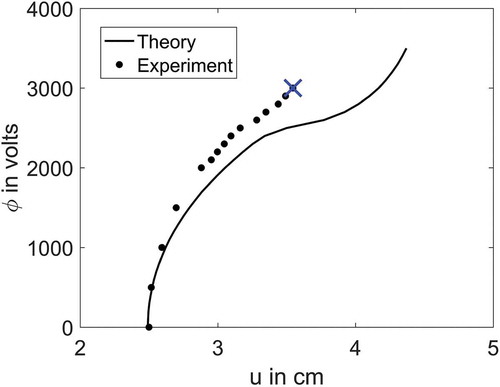
The overall shape of the DE transducer and the progression of wrinkles from the inner to outer ring observed in experiment is captured by the analytical model (Figure 8). Loss of tension happens at a higher voltage in experiment compared to the theoretical prediction. This may be due to the decrease in permittivity at a higher stretch and the resulting lower Maxwell stress [31]. The proposed analytical model doesn’t account for the change in permittivity with stretch. Theoretical and experimental plots of voltage versus displacement are given in Figure 9. The deviation between these can also be accounted for the decrease in permittivity at higher stretches.

Figure 8. Comparison of deformed shape from theoretical prediction and experimental observation.

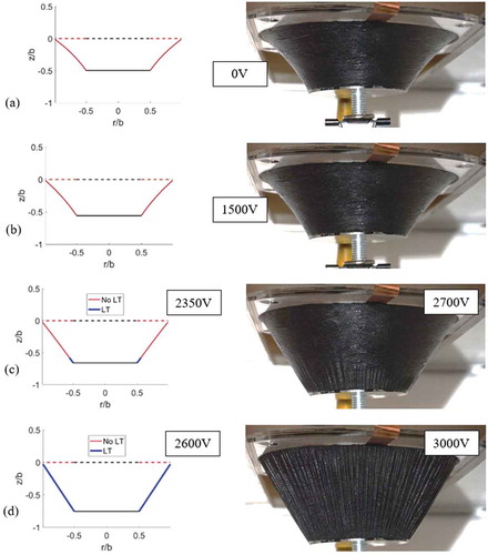
Figure 9. Voltage vs displacement plot. Blue cross indicates the point of electric breakdown.

Operational boundaries and maximum energy

We now create plots of maps with limiting boundaries denoted by mechanical rupture, electrical breakdown, zero electric field, loss of tension and minimum capacitance (Figure 10). The area calculated from Figure 10 is the non dimensionalized energy, The specific energy can be calculated as,

(15)

Figure 10. Operational boundaries of loudspeaker DEG. Green curve is the curve for zero electric field, red is the rupture curve, blue is the electric breakdown curve, black line is the minimum capacitance line and the cyan curve is the s₂ = 0 line. The light grey area is the allowable states if we consider loss of tension as an operational limit. Dark grey area is the allowable states post tension loss. For force displacement diagram this region is narrow. A:B = 0.5 and λ_p = 2.

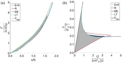
is the density and V is the volume of the elastomer. The value of used for the analysis is 960Kg/m³ (obtained from the datasheet of VHB 4905).

Area bounded by all the operational boundaries gives the maximum non-dimensionalized energy output. This is represented by the light grey area in the Figure 10. For the selected prestretch and A to B ratio it is 0.395 which is an equivalent of, 219mJ/g. DE can still be operated beyond loss of tension. The area including post tension loss is found to be 0.411, which is an equivalent of, 228mJ/g. This is the combined area of light and dark grey area in Figure 10. Hence the increase in energy beyond loss of tension is, about 4%. But this quantity is dependent on material limits, to be further explained in section, Boundaries of a hypothetical elastomer.

Optimizing maximum energy by geometry and pre-stretch

In this section, we will analytically determine the inner-outer ring ratio and equal biaxial prestretch that maximize the energy of conversion. It is intuitive that the maximum energy is affected by the inner-outer ring ratio, and the amount of initial pre-stretch that we apply on the DE membrane. We seek to understand the effect of these two parameters as follows: The inner-to-outer ring ratio (A:B) varies between 0 and 1. For A:B → 0, the out-of-plane force will act at a point, leading to singularity of stress concentration [32]. For A:B → 1, there is no material to deform. Hence, we expect an optimal ratio that will maximize the energy.

The DE membrane must be pre-stretched to delay the formation of wrinkles. Early formation of wrinkles leads to localized thinning of membrane, which may lead to dielectric breakdown. A membrane with no pre-stretch develops wrinkles immediately, and hence, we expect the energy to be small. A membrane that is highly pre-stretched will be pushed too close to the point of rupture, severely limiting any further deformation. By this token, we also expect an optimal pre-stretch that maximizes energy, we vary both the inner-to-outer ring ratio and the pre-stretch, to find the maximum non-dimensionalized energy (Figure 11) and specific energy (Figure 12). Non-dimensionalized energy provides a measure of total energy per unit plan area, normalized by the small-strain shear stiffness of the membrane. Figure 11 suggests a non-geometry and material sensitive optimized inner-to-outer ring ratio of between 0.5 and 0.6. The specific energy plot shows an optimal pre-stretch of around 3.5 for any inner-to-outer ring ratio, for the specific material VHB used in our analysis. As the inner-to-outer ring ratio increases, Figure 12 suggests a monotonic increase in specific energy. This is because as the ratio increases, the active membrane material reduces. In the limit when the ratio is 1, there is physically no material left in between the rings; the mass becomes negligible. As the ratio approaches 1, the deformation between the rings will exhibit less inhomogeneity, but it is theoretically still able to deform and convert energy. This means that for large ring ratios, the specific energy would approach a finite maximum.

Figure 11. Non-dimensionalized energy vs A:B and λ_p. (a) is plotted with s₂ = 0 as a limit – the DE is always operating in a non-wrinkled flat configuration and (b) exploits deformation post tension loss, with a small enhancement of energy of conversion in the region of low prestretch.

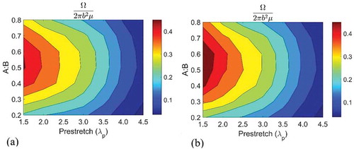
Figure 12. Specific energy vs A:B and λ_p. (a) is plotted with s₂ = 0 as a limit – the DE is always operating in a non-wrinkled flat configuration and (b) exploits deformation post tension loss.

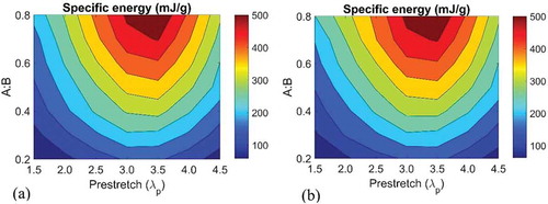
Figure 11 allows one to maximize energy output for any elastomer by using an inner-to-outer ring geometry in the vicinity of 0.5. On the other hand, if one simply desires to maximize the specific energy, a pre-stretch of 3.5 is needed on a VHB and construct a ring-like geometry with very high ring ratios. This framework allows one to analyse and optimize DE membranes of loudspeaker configuration made of different materials.

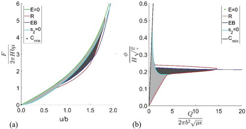
Boundaries of a hypothetical elastomer

Consider a material with a rupture parameter of and electric breakdown strength, MV/m. This is equivalent to an electric field strength of 7 when non-dimensionalized using . The permittivity and small strain shear modulus used for non-dimensionalization are of VHB 4905 described before. The operational boundaries evaluated for this hypothetical elastomer for a prestretch of 2 and A to B ratio of 0.5 is given in Figure 13. Area bounded by all the operational boundaries is 0.46 which is an equivalent of, 256mJ/g and the same calculated for all the operational boundaries excluding the loss of tension line is 0.72 which is an equivalent of, 400mJ/g. This is an increase of 57%. Hence an elastomer of large enough rupture limit and electric breakdown strength can be operated beyond loss of tension to harvest a much larger amount of energy.

Figure 13. Operational boundaries of a hypothetical elastomer whose rupture limit, J_R = 0.6 J_lim and electric breakdown strength, E√(ε/μ) = 7. A:B = 0.5 and λ_p = 2.

Conclusion

We propose a method to plot operational boundaries of a DE subject to non-homogeneous deformation. The limits of operation prescribe an allowable region of operation on a work-conjugate plot. The area bounded by the allowable region gives the maximum energy of conversion, and one may design cycles of operation within this region. We choose loudspeaker configuration to illustrate our method. Our analysis revealed that the classical electromechanical instability does not affect the DE in such a configuration, as the displacement of the DE varies monotonically with voltage. We further found that the DE remains operational even after tension loss in the hoop direction. Using these observations, we determine the inner-to-outer ring ratio and pre-stretch that maximizes energy of conversion.

Our analysis demonstrates a method to model all possible states of a DE subject to non-homogeneous deformation. This same framework could be adopted for any other dielectric elastomers undergoing non-homogeneous deformation, hopefully revealing more interesting physics in the field of dielectric elastomers.

Acknowledgements

This research was supported through funding from the 1st grant call under the Joint Science and Technology Research Cooperation between the Department of Science & Technology (DST), Govt. of India and the Agency for Science, Technology and Research (A*STAR). SJAK wishes to acknowledge the A*STAR-DST grant no. R-265-000-524-305 (SERC 142 520 3140) for funding this research. Anup Teejo Mathew also wishes to acknowledge the NUS Research Scholarship for PhD study in NUS from August 2015 to August 2019

Disclosure statement

No potential conflict of interest was reported by the authors.

Supplementary Material

Supplemental data for this article can be accessed here.

Additional information

Funding

This work was supported by the Agency for Science, Technology and Research (Singapore) and Department of Science & Technology (India) (A*STAR-DST) [R-265-000-524-305 (SERC 142 520 3140)];

References

- R. Pelrine, R.D. Kornbluh, J. Eckerle, P. Jeuck, S. Oh, Q. Pei, and S. Stanford, Dielectric elastomers: Generator mode fundamentals and applications, SPIE’s 8th Annual International Symposium on Smart Structures and Materials. pp. 148–156, 2001. doi: 10.1117/12.432640
- G. Kofod, P. Sommer-Larsen, R. Kornbluh, and R. Pelrine, Actuation response of polyacrylate dielectric elastomers, J. Intell. Mater. Syst. Struct. 14 (12) (2003), pp. 787–793. doi:10.1177/104538903039260
- R.E. Pelrine, R.D. Kornbluh, and J.P. Joseph, Electrostriction of polymer dielectrics with compliant electrodes as a means of actuation, Sensors Act A: Phys., 64, 1 (1998), pp. 77–85. doi:10.1016/s0924-4247(97)01657-9
- R. Pelrine, High-speed electrically actuated elastomers with strain greater than 100%, Science, 287, 5454 (2000), pp. 836–839. doi:10.1126/science.287.5454.836
- J. Huang, S. Shian, Z. Suo, and D.R. Clarke, Maximizing the energy density of dielectric elastomer generators using equi-biaxial loading, Adv. Funct. Mater., 23, 40 (2013), pp. 5056–5061. doi:10.1002/adfm.201300402
- J. Zhu, M. Kollosche, T. Lu, G. Kofod, and Z. Suo, Two types of transitions to wrinkles in dielectric elastomers, Soft Matter, 8, 34 (2012), pp. 8840. doi:10.1039/c2sm26034d
- G. Kovacs, L. Düring, S. Michel, and G. Terrasi, Stacked dielectric elastomer actuator for tensile force transmission, Sensors Act A: Phys., 155, 2 (2009), pp. 299–307. doi:10.1016/j.sna.2009.08.027
- T. Lu, C. Chiang Foo, J. Huang, J. Zhu, and Z. Suo, Highly deformable actuators made of dielectric elastomers clamped by rigid rings, J. Appl. Phys., 115, 18 (2014), pp. 184105. doi:10.1063/1.4876722
- T. He, X. Zhao, and Z. Suo, Dielectric elastomer membranes undergoing inhomogeneous deformation, J. Appl. Phys., 106, 8 (2009), pp. 083522. doi:10.1063/1.3253322
- G. Moretti, M. Fontana, and R. Vertechy, Parallelogram-shaped dielectric elastomer generators: Analytical model and experimental validation, J. Intell. Mater. Syst. Struct., 26, 6 (2014), pp. 740–751. doi:10.1177/1045389x14563861
- S.J.A. Koh, X. Zhao, and Z. Suo, Maximal energy that can be converted by a dielectric elastomer generator, Appl. Phys. Lett., 94, 26 (2009), pp. 262902. doi:10.1063/1.3167773
- Y. Liu, L. Liu, Z. Zhang, Y. Jiao, S. Sun, and J. Leng, Analysis and manufacture of an energy harvester based on a Mooney-Rivlin–Type dielectric elastomer, EPL (Europhysics Letters), 90, 3 (2010), pp. 36004. doi:10.1209/0295-5075/90/36004
- L. Xiongfei, L. Liwu, L. Yanju, and L. Jinsong, Dielectric elastomer energy harvesting: Maximal converted energy, viscoelastic dissipation and a wave power generator, Smart Mater. Struct., 24, 11 (2015), pp. 115036. doi:10.1088/0964-1726/24/11/115036
- Z. Suo, X. Zhao, and W. Greene, A nonlinear field theory of deformable dielectrics, J. Mech. Phys. Solids, 56, 2 (2008), pp. 467–486. doi:10.1016/j.jmps.2007.05.021
- N. Bonwit, J. Heim, M. Rosenthal, C. Duncheon, and A. Beavers, Design of commercial applications of EPAM technology, Smart Struct. Mat., (2006), pp. 616805–616805-10. doi:10.1117/12.658775.
- H.-M. Wang, J.-Y. Zhu, and K.-B. Ye, Simulation, experimental evaluation and performance improvement of a cone dielectric elastomer actuator, J. Zhejiang Uni. -SCIENCE A, 10, 9 (2009), pp. 1296–1304. doi:10.1631/jzus.A0820666
- S. Hau, G. Rizzello, M. Hodgins, A. York, and S. Seelecke, Design and control of a high-speed positioning system based on dielectric elastomer membrane actuators, IEEE/ASME Transact. Mechat., 22, 3 (2017), pp. 1259–1267. doi:10.1109/tmech.2017.2681839
- V.K.V. Tran, M.A. Teejo, and S.J.A. Koh, Stackable configurations of artificial muscle modules that is continuously-tunable by voltage, SPIE Smart Structures and Materials+ Nondestructive Evaluation and Health Monitoring. pp. 101632K-101632K-12, 2017. doi: 10.1117/12.2261787
- E. Bortot and M. Gei, Harvesting energy with load-driven dielectric elastomer annular membranes deforming out-of-plane, Extr. Mech. Let., 5 (2015), pp. 62–73. doi:10.1016/j.eml.2015.09.009
- T. McKay, B. O’Brien, E. Calius, and I. Anderson, Self-priming dielectric elastomer generators, Smart Mater. Struct., 19, 5 (2010), pp. 055025. doi:10.1088/0964-1726/19/5/055025
- T.G. McKay, B.M. O’Brien, E.P. Calius, and I.A. Anderson, Soft generators using dielectric elastomers, Appl. Phys. Lett., 98, 14 (2011), pp. 142903. doi:10.1063/1.3572338
- T.E. Tezduyar, L.T. Wheeler, and L. Graux, Finite deformation of a circular elastic membrane containing a concentric rigid inclusion, Int. J. Non Linear Mech., 22, 1 (1987), pp. 61–72. doi:10.1016/0020-7462(87)90049-7
- T. He, Y. Li, H. Li, and C. Chen, Optimization design for a dielectric elastomer membrane actuator, Int. J. Computational Mater. Sci. Eng., 02, 01 (2013), pp. 1350002. doi:10.1142/s2047684113500024
- S. Seifi and H.S. Park, Electro-elastocapillary Rayleigh-plateau instability in dielectric elastomer films, Soft Matter, 13, 23 (2017), pp. 4305–4310. doi:10.1039/C7SM00917H
- T. Li, C. Keplinger, R. Baumgartner, S. Bauer, W. Yang, and Z. Suo, Giant voltage-induced deformation in dielectric elastomers near the verge of snap-through instability, J. Mech. Phys. Solids, 61, 2 (2013), pp. 611–628. doi:10.1016/j.jmps.2012.09.006
- L. Liu, Y. Liu, X. Luo, B. Li, and J. Leng, Electromechanical instability and snap-through instability of dielectric elastomers undergoing polarization saturation, Mech. Mater., 55 (2012), pp. 60–72. doi:10.1016/j.mechmat.2012.07.009
- T. Lu, J. Huang, C. Jordi, G. Kovacs, R. Huang, D.R. Clarke, and Z. Suo, Dielectric elastomer actuators under equal-biaxial forces, uniaxial forces, and uniaxial constraint of stiff fibers, Soft Matter, 8, 22 (2012), pp. 6167. doi:10.1039/c2sm25692d
- S. Colonnelli, G. Saccomandi, and G. Zurlo, The role of material behavior in the performances of electroactive polymer energy harvesters, J. Polym. Sci., Part B: Polym. Phys., 53, 18 (2015), pp. 1303–1314. doi:10.1002/polb.23761
- J. Huang, S. Shian, R.M. Diebold, Z. Suo, and D.R. Clarke, The thickness and stretch dependence of the electrical breakdown strength of an acrylic dielectric elastomer, Appl. Phys. Lett., 101, 12 (2012), pp. 122905. doi:10.1063/1.4754549
- S.J.A. Koh, C. Keplinger, R. Kaltseis, -C.-C. Foo, R. Baumgartner, S. Bauer, and Z. Suo, High-performance electromechanical transduction using laterally-constrained dielectric elastomers part I: Actuation processes, J. Mech. Phys. Solids, 105 (2017), pp. 81–94. doi:10.1016/j.jmps.2017.04.015
- M. Wissler and E. Mazza, Electromechanical coupling in dielectric elastomer actuators, Sensors Act A: Phys., 138, 2 (2007), pp. 384–393. doi:10.1016/j.sna.2007.05.029
- S. Timoshenko, On stresses in a plate with a circular hole, J. Franklin Inst., 197, 4 (1924), pp. 505–516. doi:10.1016/s0016-0032(24)90690-9