Simulation of vessel tissue remodeling with residual stress: an application to in-stent restenosis

ABSTRACT

We present a numerical procedure to model the artery wall remodeling stimulated by stenting considering varying degree of residual stresses. This framework sets up biological remodeling with the existence of residual stress. Previous studies suggest that the residual stress originates from the growth and remodeling of the premature tissue. Meanwhile, it is known that tissue remodeling can happen under mechanical loading. However, none of the existing research studies the impact of residual stress on the mechanical-driven growth of biomaterials. To fill this gap, we build a numerical framework that couples the residual stress with a growth model, and examine its impact on tissue remodeling. The proposed approach is applied to in-stent restenosis, where the tissue remodeling process is modeled with finite element method, and the residual stress is generated geometrically using open angle method. The result shows that residual stress reverses the radial distribution of stress concentration, which is ameliorated by tissue remodeling. The thickening of vessel wall tends to increase with residual stress, which links to more severe in-stent restenosis. The results demonstrate the important interplay between residual stress and tissue remodeling. The findings suggest that residual stress should be considered in the future simulation of tissue remodeling.

KEYWORDS:

• Residual stress
• remodeling
• growth model
• in-stent restenosis

1. Introduction

The residual stress in biological soft tissues has been known to exist. In the well-known cutting experiment [1], Fung demonstrates the existence of residual stress in arteries, and postulates that residual stress is generated from the remodeling of artery tissue during its growth. Since then, a variety of research has been done to investigate the origin of it. Based on clinical observations, Richman et al. [2], speculates that cortical folding in the brain results from the stress induced by differential or constrained growth. Similarly, it is demonstrated in [3] through experiments that uncontrolled growth of cancer cells within confined tissue space also generates residual stress, which is a signal to stop replicating but has been ignored by the cancer cells. Several other studies also interpret residual stress as the result of tissue growth [4–6].

However, the impact of residual stress on tissue remodeling and growth remains unanswered. It is known that tissue growth and remodeling occurs after its full development, upon external mechanical loading [7]. Growth and remodeling act as a response to environmental changes, which can be driven by many factors such as nutrient, hormon, growth factor, stress and so on. In this manuscript, only mechanical-driven growth is discussed, and the scale of the modeling is on macro level, from the viewpoint of continuum, not on the level of individual cells or genes. Therefore the model is essentially ‘phenomenological’, which does not explain the fundamental biological mechanisms. For instance, the concept of mechanical-driven isotropic growth has been utilized in pediatric forehead reconstruction by inserting a silicon balloon expander which stimulates skin growth [8]. It is natural to ask: does residual stress play a role in the growth process? Research evidence shows residual stress significantly changes the stress distribution as well as the mechanical properties in tissues [26-28] . It is therefore reasonable to assume that the existence of residual stress affects the mechanical-driven growth of tissues, although the existing growth models fail to account for this important factor.

The main issues we try to address in this paper is to bridge the relationship between residual stress and tissue remodeling by showing that residual stress may also affect tissue remodeling under external mechanical loading. To accomplish this, we will model and characterize mechanical-driven remodeling using varying degree of residual stress. To load the vessel with residual stress, we will use open angle method proposed in [1], which is widely used as a phenomenological model to approximate the in vivo residual stress distribution. To model the vessel wall remodeling or growth, a stress-modulated growth model based on the multiplicative decomposition of kinematics is used. Modeling vessel growth using continuum mechanics approach is effective in several vessel applications in recent years Himpel et al. [9], Kuhl et al. [10]. Assuming isotropic growth, we extend the baseline hyperelastic model with an additional scalar: growth factor. The stress and elasticity tensors are functions of the growth factor and the growth factor is governed by a stress-modulated law. Comparing to other numerical models to study tissue remodeling such as the mixture theory [4], the multiplicative decomposition approach has simpler governing equations and can be easily generalized and coupled with other existing modeling frameworks.

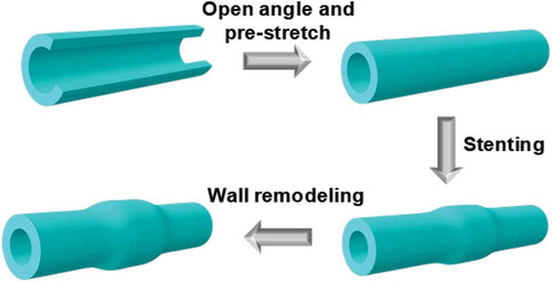
As an application of the effect of residual stress on biological tissue remodeling, we investigate the vessel wall remodeling caused by stenting. In a stent procedure, the stenosed blood vessel is expanded by a stent – a system of tiny struts. Meanwhile the compression of the plaque usually comes with trauma to the blood vessel wall. Physiologically, a blood clot often forms at the site of trauma, which is accompanied by an inflammatory immune response. Then, 3 – 6 months after the surgery, the endothelial cells proliferate as a healing process. This proliferation of endothelial cells results in the wall thickening and sometimes when it becomes excessive, the cells can obstruct the blood vessel at the site of the stent [11], which is called restenosis. Phenomenologically, the remodeling of the vessel tissue can be described as ‘mechanical-driven isotropic growth’. Our goal is to simulate the impact of the residual stress on the growth of artery stimulated by the placement of a stent. As a preliminary study, we model the placement of the stent as a prescribed radial displacement. The simulation process of the in-stent restenosis is illustrated in Figure 1. It starts with a pre-stretch of the vessel to generate residual stress, stenting procedure is then imposed where mechanical loading is applied on the inner wall of the artery, the combined residual stress and mechanical load provide an updated distribution of stress and tissue remodeling occurs.

Figure 1. Schematics of the simulation process.

The remainder of the paper is organized as follows: in Section 2 we briefly review the geometric open-angle method we used to generate residual stress, the stress-driven growth model to simulate the vessel remodeling or growth, and the framework procedure summary that couples the residual stress with the stress-driven growth model. In Section 3, the setup of the in-stent restenosis study is described. The results and discussions are presented in Section 4. Finally, conclusions are drawn in Section 5.

2. Simulation and modeling approach

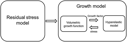
In this section, we present a coupled framework to simulate residual-stress-based tissue growth. As shown in Figure 2 the framework includes two major components: a model representing residual stress and a stress-modulated growth model that characterizes restenosis. A baseline hyperelastic model is incorporated in the growth function.

Figure 2. Computational model framework that couples the residual stress with hyperelastic stressed-based growth model.

2.1. Residual stress

In our computational framework, the residual stress is generated using open-angle method. Using the open-angle method, the vessel is assumed to have an open angle in its stress-free state. The vessel is then subjected to an axial pre-stretch and bent into a full tube, thus becoming stressed. The use of open angle and pre-stretch is inspired by the circumferential and longitudinal development of premature vessel tissue and has been widely used to approximate the distribution of vascular residual stress. It is found to be capable of approximating the experimental observations [4,12,13].

Mathematically speaking, consider an arbitrary point $(R,\mathrm{\Theta },Z)$ in a cylindrical coordinate system, assume it moves to $(r,\theta ,z)$ after closing the open angle. Assuming symmetry, we denote the half open angle as $\psi$, the axial stretch ratio as ${\lambda }_z$, the original inner and outer radius as $R_{\mathrm{i}\mathrm{n}}$ and $R_{\mathrm{o}\mathrm{u}\mathrm{t}}$, and the deformed inner and outer radius as $r_{\mathrm{i}\mathrm{n}}$ and $r_{\mathrm{o}\mathrm{u}\mathrm{t}}$ respectively. The residual strain is obtained by postulating the following geometric constraints:

1. The volume does not change after the deformation:

(1) $\frac{\pi -\psi }{\pi }({R_{\mathrm{o}\mathrm{u}\mathrm{t}}}^2-{R_{\mathrm{i}\mathrm{n}}}^2)={\lambda }_z({r_{\mathrm{o}\mathrm{u}\mathrm{t}}}^2-{r_{\mathrm{i}\mathrm{n}}}^2)$(1)

2. The radial, circumferential and axial strain are constant:

(2) ${ϵ}_{rr}=\frac{\mathrm{\partial }{u}_r}{\mathrm{\partial }r}=\mathrm{c}\mathrm{o}\mathrm{n}\mathrm{s}\mathrm{t}$(2)

(3) ${ϵ}_{\theta \theta }=\frac{1}{r}\frac{\mathrm{\partial }{u}_r}{\mathrm{\partial }\theta }+\frac{u_r}{r}=\mathrm{c}\mathrm{o}\mathrm{n}\mathrm{s}\mathrm{t}$(3)

(4) ${ϵ}_{zz}=\frac{\mathrm{\partial }{u}_z}{\mathrm{\partial }z}=\mathrm{c}\mathrm{o}\mathrm{n}\mathrm{s}\mathrm{t}$(4)

Using Equations (1)-(4), for a given half open angle $\psi$ we can map the new ‘closed-vessel’ coordinates as functions of the original ‘open-angle’ coordinates:

(5a) $r=R\sqrt{\frac{\pi -\psi }{\pi {\lambda }_z}}$(5a)

(5b) $z={\lambda }_{z}Z$(5b)

(5c) $\theta =\mathrm{\Theta }-\frac{\mathrm{\Theta }-\pi }{\psi -\pi }\psi$(5c)

With the residual strain or the deformation explicitly obtained, we are able to evaluate residual stress distribution of the artery for each discrete point in the computational model using a given constitutive equation for the material description.

2.2. Growth model with baseline hyperelasticity

In recent two decades, finite element method has been successfully applied to model tissue growth and remodeling. One of the early attempts of a computational growth method is applied to vessels in [6], where a simple phenomenological model is adopted to study the interrelations between growth model with growth parameters and growth-induced residual stresses in arteries. Despite the simplicity of this model, it is able to demonstrate the interdependency between tissue growth and residual stress. Similarly, Olsson and Klarbring [5], developed a thermodynamically consistent model for growth and remodeling in elastic arteries specialized for cylindrical geometry. Admitting that the method is phenomenological, the authors conclude that such a method is able to predict the stress distribution in the vessel and can be extended to solve other problems such as aneurysm development. Klarbring et al. [14], extends the multiplicative decomposition approach to hyperelastic materials and formulated the arterial remodeling as a boundary value problem of nonlinear elasticity. By decomposing the deformation gradient into an elastic part and a growth part, this approach identifies an intermediate configuration which does not have to be compatible [15–17].

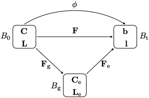
The key idea of the kinematics of the growth model is the multiplicative decomposition of deformation gradient $\mathbf{F}$ into an elastic part ${\mathbf{F}}_{\mathrm{e}}$ and a growth part ${\mathbf{F}}_{\mathrm{g}}$. Based on the work in [9,18], an intermediate configuration $B_{\mathrm{g}}$ is introduced between the reference configuration $B_0$ and the current configuration $B_{\mathrm{t}}$. As shown in Figure 3, $\chi$ is the mapping from $B_0$ to $B_{\mathrm{t}}$, and the deformation gradient $\mathbf{F}$ is defined in regular way as $\mathbf{F}=\mathrm{\partial }\chi /\mathrm{\partial }\mathbf{X}$. We assume there exists a decomposition:

(6) $\mathbf{F}={\mathbf{F}}_{\mathrm{e}}\cdot {\mathbf{F}}_{\mathrm{g}}$(6)

Figure 3. Multiplicative decomposition of the deformation gradient $\mathbf{F}$ in the growth model: intermediate configuration with growth and elastic components.

Similarly, the right Cauchy-Green tensor $\mathbf{C}$, velocity gradient $\mathbf{l}$, Piola-Kirchhoff stress $\mathbf{P}$ and the second Piola-Kirchhoff (PK2) stress $\mathbf{S}$ can be decomposed into elastic and growth parts as well. Let ${\rho }_0$ denote the density in the reference configuration, ${\rho }_{\mathrm{t}}$ and ${\rho }_{\mathrm{g}}$ denote its counterparts in the spatial configuration and the intermediate configuration, respectively. Define the volume of a material particle in the reference, spatial and intermediate configurations as $dV$, $dv$ and $d{V}_{\mathrm{g}}$, respectively. In analogy to $J=\mathrm{d}\mathrm{e}\mathrm{t}\mathbf{F}$, define the Jacobians $J_{\mathrm{e}}=\mathrm{d}\mathrm{e}\mathrm{t}{\mathbf{F}}_{\mathrm{e}}$ and $J_{\mathrm{g}}=\mathrm{d}\mathrm{e}\mathrm{t}{\mathbf{F}}_{\mathrm{g}}$. The transformations of the volumes become:

(7) $dv=JdV,d{V}_{\mathrm{g}}=J_{\mathrm{g}}dV,dv=J_{\mathrm{e}}d{V}_{\mathrm{g}}$(7)

and

(8) $J=J_{\mathrm{e}}{J}_{\mathrm{g}}$(8)

Based on the definitions, we have the following density transformations:

(9) ${\rho }_{\mathrm{g}}d{V}_{\mathrm{g}}={\rho }_{\mathrm{t}}dv,{\rho }_{\mathrm{g}}=J_{\mathrm{e}}{\rho }_{\mathrm{t}}$(9)

For soft tissues, it is typically assumed density remains constant upon growth, which means ${\rho }_{\mathrm{g}}=\mathrm{c}\mathrm{o}\mathrm{n}\mathrm{s}\mathrm{t}$ and ${\dot{\rho }}_{\mathrm{g}}=0$. However, the density in the reference configuration changes, due to the increased mass and fixed volume. The increased density in the reference configuration is denoted as as ${\bar{\rho }}_0$, which is related to the densities in the spatial configuration and intermediate configuration by ${\bar{\rho }}_0=J{\rho }_{\mathrm{t}}=J_{\mathrm{g}}{\rho }_{\mathrm{g}}$. Furthermore, the change of ${\bar{\rho }}_0$ is assumed to be driven by a mass source $R_0$:

(10) ${\dot{\bar{\rho }}}_0=R_0$(10)

The derivative of ${\bar{\rho }}_0$ in Equation 10 can be evaluated as ${\bar{\rho }}_0\mathrm{t}\mathrm{r}{\mathbf{L}}_{\mathrm{g}}$ where ${\mathbf{L}}_{\mathrm{g}}$ is the growth part of velocity gradient, and can be easily determined by the growth tensor ${\mathbf{F}}_{\mathrm{g}}$.

The growth process is assumed to be quasi-static, therefore the linear momentum balance is simply:

(11) $\mathrm{d}\mathrm{i}\mathrm{v}\mathit{\sigma }=0$(11)

Denote the Helmholtz free energy of the hyperelastic material as $\mathrm{\Psi }(\mathbf{C},{\mathbf{F}}_{\mathrm{g}})$, the PK2 stress and Kirchhoff stress can be evaluated as:

(12a) $\mathbf{S}=2\frac{\mathrm{\partial }\mathrm{\Psi }}{\mathrm{\partial }\mathbf{C}}=2\frac{\mathrm{\partial }\mathrm{\Psi }}{\mathrm{\partial }{\mathbf{C}}_{\mathrm{e}}}:\frac{\mathrm{\partial }{\mathbf{C}}_{\mathrm{e}}}{\mathrm{\partial }C}={\mathbf{F}}_{\mathrm{g}}^{-1}\cdot {\mathbf{S}}_{\mathrm{e}}\cdot {\mathbf{F}}_{\mathrm{g}}^{-T}$(12a)

(12b) $\mathit{\tau }=\mathbf{F}\cdot \mathbf{S}\cdot {\mathbf{F}}^T={\mathbf{F}}_{\mathrm{e}}\cdot {\mathbf{S}}_{\mathrm{e}}\cdot {\mathbf{F}}_{\mathrm{e}}^T$(12b)

where ${\mathbf{S}}_{\mathrm{e}}$ denotes the elastic part of $\mathbf{S}$. The constitutive moduli $\mathbb{C}$ can be obtained by taking the derivative of $\mathbf{S}$ with respect to $\mathbf{C}$, and its counterpart in the current configuration can be derived by a push-forward operation:

(13a) $\mathbb{C}=2\frac{d\mathbf{S}(\mathbf{F},{\mathbf{F}}_{\mathrm{g}})}{d\mathbf{C}}=2\frac{\mathrm{\partial }\mathbf{S}(\mathbf{F},{\mathbf{F}}_{\mathrm{g}})}{\mathrm{\partial }\mathbf{C}}{\left|{ }_{{\mathbf{F}}_{\mathrm{g}}}+2\left[\frac{\mathrm{\partial }\mathbf{S}}{\mathrm{\partial }{\mathbf{F}}_{\mathrm{g}}}:\frac{\mathrm{\partial }{\mathbf{F}}_{\mathrm{g}}}{\mathrm{\partial }{\theta }_{\mathrm{g}}}\right]\otimes \frac{\mathrm{\partial }{\theta }_{\mathrm{g}}}{\mathrm{\partial }\mathbf{C}}\right|}_{\mathbf{F}}$(13a)

(13b) $ℂ=(F\overline{\otimes }F):ℂ:(F^T\overline{\otimes }{F}^T)$(13b)

It can be seen immediately from Equations (12) and (13) that both the stress and its moduli differ from their usual form only by an additional variable ${\mathbf{F}}_{\mathrm{g}}$, which is determined independently by the governing equation of the growth. This resembles the concept of plasticity in the sense that the basic constitutive equations themselves remain unchanged. However, they are evaluated exclusively in terms of the kinematic quantities of the intermediate configuration.

To complete the stress and constitutive moduli, the growth deformation tensor ${\mathbf{F}}_{\mathrm{g}}$ must be uniquely determined. It can be either isotropic or anisotropic, we adopt a simple isotropic form:

(14) ${\mathbf{F}}_{\mathrm{g}}={\theta }_{\mathrm{g}}\mathbf{I}$(14)

where ${\theta }_{\mathrm{g}}$ denotes an internal variable which is often referred to as growth factor. The growth multipliers are $1$ in the plain elastic deformation, greater than $1$ in growth, and smaller than $1$ in atrophy.

To model the evolution of the growth multipliers, the rate of growth multipliers are usually specified as:

(15) ${\dot{\theta }}_{\mathrm{g}}=k_{\mathrm{g}}({\theta }_{\mathrm{g}})\cdot {\varphi }_{\mathrm{g}}({\mathbf{F}}_{\mathrm{e}})$(15)

where ${\varphi }_{\mathrm{g}}$ is a growth criterion function to enforce a threshold on the growth, $k_{\mathrm{g}}$ is a weighted function to prevent unlimited growth. ${\varphi }_{\mathrm{g}}$ and $k_{\mathrm{g}}$ are specified with the following forms in [9] with detailed parameter studies:

(16a) ${\varphi }_{\mathrm{g}}=\mathrm{t}\mathrm{r}({\mathbf{M}}_{\mathrm{e}})-M_{\mathrm{e}}^{\mathrm{c}\mathrm{r}\mathrm{i}\mathrm{t}}$(16a)

(16b) $k_{\mathrm{g}}=\frac{1}{\tau }{\left(\frac{{\theta }_{\mathrm{m}\mathrm{a}\mathrm{x}}-{\theta }_{\mathrm{g}}}{{\theta }_{\mathrm{m}\mathrm{a}\mathrm{x}}-1}\right)}^{\gamma }$(16b)

where $\tau$ and $\gamma$ are material constants that are used to control the speed of growth, ${\mathbf{M}}_{\mathrm{e}}$ is the Mandel stress defined as ${\mathbf{M}}_{\mathrm{e}}={\mathbf{C}}_{\mathrm{e}}\cdot {\mathbf{S}}_{\mathrm{e}}$, and $M_{\mathrm{e}}^{\mathrm{c}\mathrm{r}\mathrm{i}\mathrm{t}}$ is the criterion of growth.

A local Newton iteration is used to solve for the growth factor. Applying backward Euler scheme to Equation (15), we have:

(17) ${\dot{\theta }}_{\mathrm{g}}=({\theta }_{\mathrm{g}}-{\theta }_{\mathrm{g}}^n)/\mathrm{\Delta }t$(17)

and the residual is evaluated as:

(18) $R={\theta }_{\mathrm{g}}-{\theta }_{\mathrm{g}}^{\mathrm{n}}-\frac{1}{\tau }{\left(\frac{{\theta }_{\mathrm{m}\mathrm{a}\mathrm{x}}-{\theta }_{\mathrm{g}}}{{\theta }_{\mathrm{m}\mathrm{a}\mathrm{x}}-1}\right)}^{\gamma }\left(\mathrm{t}\mathrm{r}({\mathbf{M}}_{\mathrm{e}})-M_{\mathrm{e}}^{\mathrm{c}\mathrm{r}\mathrm{i}\mathrm{t}}\right)\mathrm{\Delta }t$(18)

To minimize the residual $R$, we linearize Equation (18) for the tangent modulus $K$:

(19) $K=\frac{\mathrm{\partial }R}{\mathrm{\partial }{\theta }_{\mathrm{g}}}=1-\left(k_{\mathrm{g}}\frac{\mathrm{\partial }{\varphi }_{\mathrm{g}}}{\mathrm{\partial }{\theta }_{\mathrm{g}}}+{\varphi }_{\mathrm{g}}\frac{\mathrm{\partial }{k}_{\mathrm{g}}}{\mathrm{\partial }{\theta }_{\mathrm{g}}}\right)\mathrm{\Delta }t$(19)

In the local Newton iteration, where the deformation tensor $\mathbf{F}$ is known, the stretch ratio ${\theta }_{\mathrm{g}}$ is updated with ${\theta }_{\mathrm{g}}\leftarrow {\theta }_{\mathrm{g}}-R/K$. The corresponding growth part of the deformation tensor ${\mathbf{F}}_{\mathrm{g}}$ can be calculated using Equation (14). Consequently the elastic part ${\mathbf{F}}_{\mathrm{e}}$ can be calculated with Equation (6). Then the elastic stress ${\mathbf{S}}_{\mathrm{e}}$ and elastic constitutive moduli ${\mathbb{C}}_{\mathrm{e}}$ can be obtained with Equations (12) and (13) respectively.

Compressible Neo-Hookean is used as the baseline hyperelastic model since it has been validated in multiple applications such as [9,10,18,19]. But there is no fundamental difficulty preventing other models being used. The specific form of the free energy is written as:

(20) $\mathrm{\Psi }=\frac{\lambda }{2}\mathrm{l}{\mathrm{n}}^2{J}_{\mathrm{e}}+\frac{1}{2}\mu \left[{\mathbf{C}}_{\mathrm{e}}:\mathbf{I}-3-2\mathrm{l}\mathrm{n}{J}_{\mathrm{e}}\right]$(20)

where $\mu$ and $\lambda$ are the Lamé parameters. The stress and constitutive moduli can be obtained based on Equation (20):

(21a) ${\mathbf{S}}_{\mathrm{e}}=\left[\lambda \mathrm{l}\mathrm{n}{J}_{\mathrm{e}}-\mu \right]{\mathbf{C}}_{\mathrm{e}}^{-1}+\mu \mathbf{I}$(21a)

(22b) ${\mathit{\tau }}_{\mathrm{e}}=(\lambda \mathrm{l}\mathrm{n}{J}_{\mathrm{e}}-\mu )\mathbf{I}+\mu {\mathbf{B}}_{\mathrm{e}}$(22b)

and

(22a) ${ℂ}_{\text{e}}=(\mu -\lambda \text{ln}{J}_{\text{e}})(C_{\text{e}}^{-1}\overline{\otimes }{C}_{\text{e}}^{-1}+C_{\text{e}}^{-1}\underset{\_}{\otimes }{C}_{\text{e}}^{-1})+\lambda C_{\text{e}}^{-1}\otimes C_{\text{e}}^{-1}$(22a)

(22b) $c_{\mathrm{e}}=(\mu -\lambda \mathrm{l}\mathrm{n}{J}_{\mathrm{e}})({\delta }_{ik}{\delta }_{jl}+{\delta }_{il}{\delta }_{jk})+\lambda {\delta }_{ij}{\delta }_{kl}$(22b)

where the operation $\bar{\otimes }$ and $\underset{\_}{\otimes }$ between two second order tensors $\mathbf{A}$ and $\mathbf{B}$ are defined as $(\mathbf{A}\bar{\otimes }\mathbf{B}{)}_{ijkl}={\mathbf{A}}_{ik}{\mathbf{B}}_{jl}$ and $(\mathbf{A}\underset{\_}{\otimes }\mathbf{B}{)}_{ijkl}={\mathbf{A}}_{il}{\mathbf{B}}_{jk}$ respectively. For more details of the mathematics in continuum mechanics, please refer to [20,21].

For completeness, we list the specific expressions of Equations (12) and (13) using compressible Neo-Hookean as the baseline hyperelasticity, the detailed derivation can be found in [18]:

(23a) $\mathbf{S}=\frac{1}{{{\theta }_{\mathrm{e}}}^2}{\mathbf{S}}_{\mathrm{e}}$(23a)

(23b) $\mathit{\tau }={\tau }_{\mathrm{e}}$(23b)

and

(24a) $\mathbb{C}=\frac{1}{{\theta }_{\mathrm{g}}^4}{\mathbb{C}}_{\mathrm{e}}-\frac{4}{{\theta }_{\mathrm{g}}^5}\frac{k_{\mathrm{g}}}{K}\mathrm{\Delta }t\left({\mathbf{S}}_{\mathrm{e}}+\frac{1}{2}{\mathbb{C}}_{\mathrm{e}}:{\mathbf{C}}_{\mathrm{e}}\right)\otimes \left(\frac{1}{2}{\mathbf{C}}_{\mathrm{e}}:{\mathbb{C}}_{\mathrm{e}}+{\mathbf{S}}_{\mathrm{e}}\right)$(24a)

(24b) $\mathbb{C}={\mathbb{C}}_{\mathrm{e}}+\frac{4}{{\theta }_{\mathrm{g}}}\frac{k_{\mathrm{g}}}{K}\mathrm{\Delta }t({\mathbf{F}}_{\mathrm{e}}\bar{\otimes }{\mathbf{F}}_{\mathrm{e}}):\left[\left({\mathbf{S}}_{\mathrm{e}}+\frac{1}{2}{\mathbb{C}}_{\mathrm{e}}:{\mathbf{C}}_{\mathrm{e}}\right)\otimes \left(\frac{1}{2}{\mathbf{C}}_{\mathrm{e}}:{\mathbb{C}}_{\mathrm{e}}+{\mathbf{S}}_{\mathrm{e}}\right)\right]:({\mathbf{F}}_{\mathrm{e}}^T\bar{\otimes }{\mathbf{F}}_{\mathrm{e}}^T)$(24b)

2.3. Algorithm and implementation

The described framework can be easily implemented within any existing nonlinear finite element framework. In the work shown here we implement it in ABAQUS CAE (Dassault Systemes, RI, USA). To apply residual stress, a ‘DISP’ subroutine is written to specify the displacement of the entire discretized finite element mesh. Since the displacement of all degrees of freedom are given, no iteration is necessary in this step. To define the growth model with baseline hyperelasticity, we use a ‘UMAT’ subroutine to specify the stress and elasticity tensors. Note that our material model involves state variables that are not available in ABAQUS such as ${\theta }_{\mathrm{g}}$, ${\mathbf{M}}_{\mathrm{e}}$, and $\tau$. They are added to the simulation as ‘SDV’. The values of ${\theta }_{\mathrm{g}}$ and ${\mathbf{M}}_{\mathrm{e}}$ are calculated in the ‘UMAT’ subroutine and the rest of the user-defined variables are entered in the Graphical User Interface (GUI). Comparing to the traditional hyperelastic models, the additional work this residual stress-based computational framework introduces is the iterative solution of the growth factor ${\theta }_{\mathrm{g}}$ and the imposition of the residual stress given discrete nodal displacement solution using open-angle approach. Algorithm 1 lists the pseudocode for the coupled algorithm.

3. Simulation setup for in-stent restenosis in a vessel

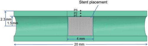
The vessel under investigation is a coronary artery. The coronary artery is modeled as a $20$mm-long 3D tube, with an inner radius of $1.5$ mm and outer radius of $2.3$ mm before expansion. The mechanical loading is the effect of the stent deployment where a uniform radial displacement is applied to the middle portion ($4$ mm) of the artery, as shown in Figure 4. By taking advantage of the symmetry, only one half of the artery is modeled. The material properties are defined as follows: $\mu =1.15385$ MPa and $\lambda =1.73077$ MPa. The growth function parameters are set to be ${\theta }_g^{\mathrm{m}\mathrm{a}\mathrm{x}}=1.5$, $M_e^{\mathrm{c}\mathrm{r}\mathrm{i}\mathrm{t}}=0$, $\gamma =5$, and $\tau =2$. The material properties and growth function parameters are first used in [10] to model patient-specific aorta. To study the influence of the residual stress on the restenosis, the simulation is partitioned into 3 steps: 1) apply residual stress with varying degree and axial stretch, 2) apply radial displacement of $0.5$ mm in the inner surface of the vessel to simulate the stent deployment, and 3) simulate in-stent restenosis, or the growth or remodeling of the artery due to stenting with the boundary conditions in step 2 unchanged. Four cases are simulated with different amount of residual stress, as listed in Table 1. The cases are designed such that Case 1 is stress-free and the others are residual-stressed. Cases 2 to 4 have different open angles and axial strains representing varying amount of residual stress in the vessel. The values of the open-angles and axial strains are in reasonable ranges as used in previous studies [6]. In all simulations, both ends of the artery are constrained in the axial or longitudinal direction, but free to expand or contract in the radial direction to allow growth.

Table 1. Cases and steps used for the simulation setup.

	Step 1	Step 2	Step 3
Case 1	no residual stress	Prescribe radial	Growth model
Case 2	open angle ${60}^{\circ }$, axial strain $1.1$	displacement of $0.3$ mm	enabled using
Case 3	open angle ${90}^{\circ }$, axial strain $1.1$	on inner surface in	parameters provided
Case 4	open angle ${60}^{\circ }$, axial strain $1.15$	the stented area.	with step 2 unchanged.

Figure 4. Geometry of the coronary artery model, the stent is placed in the middle of the model.

Algorithm 1 Pseudocode of the algorithm

1: specify displacement field to close open-angle and pre-stretch to obtain residual stress

2: specify radial displacement due to stenting to apply mechanical loading

3: for each quasi time step do

4: given $\mathbf{F}$ and ${\theta }_{\mathrm{g}}^n$

5: ${\theta }_{\mathrm{g}}\leftarrow {\theta }_{\mathrm{g}}^n$

6: while $R>tol$ do

7: compute elastic tensor ${\mathbf{F}}_{\mathrm{e}}=\mathbf{F}/{\theta }_{\mathrm{g}}$

8: compute elastic right Cauchy-Green tensor ${\mathbf{C}}_{\mathrm{e}}={\mathbf{F}}_{\mathrm{e}}^T\cdot {\mathbf{F}}_{\mathrm{e}}$

9: compute elastic second Piola-Kirchhoff stress ${\mathbf{S}}_{\mathrm{e}}$ using Equation (21a)

10: if ${\varphi }_g=\mathrm{t}\mathrm{r}({\mathbf{M}}_{\mathrm{e}})-M_{\mathrm{e}}^{\mathrm{c}\mathrm{r}\mathrm{i}\mathrm{t}}\ge 0$ then

11: compute growth function $k_{\mathrm{g}}$ using Equation (16b)

12: compute residual $R$ using Equation (18)

13: compute tangent moduli $K$ using Equation (19)

14: update growth factor ${\theta }_{\mathrm{g}}\leftarrow {\theta }_{\mathrm{g}}-R/K$

15: end if

16: end while

17: compute second Piola-Kirchhoff stress $\mathbf{S}$ using Equation (23a)

18: compute Kirchhoff stress $\tau$ using Equation (23b)

19: compute Lagrangian moduli $\mathbb{C}$ using Equation (24a)

20: compute Kirchhoff moduli $c$ using Equation (24b)

21: solve for displacement $\mathbf{u}$ and update $\mathbf{F}$

22: end for

To ensure the geometries in the pre-stenting state for the three cases are identical, we carefully choose the initial geometrical parameters, specifically inner and outer radii. This is done so that upon applying the residual stress and deformation all cases have the same geometry as in Case 1. The initial inner and outer radii in the stress-free state are listed in Table 2.

Table 2. Inner and outer radii used at the stress-free states for the 3 cases.

	$R_{\mathrm{i}\mathrm{n}}$/mm	$R_{\mathrm{o}\mathrm{u}\mathrm{t}}$/mm
Case 1	1.500	2.300
Case 2	1.723	2.642
Case 3	1.817	2.785
Case 4	1.800	2.760

A finite element mesh of $12,000$ hexahedral elements is used, with $5$ nodes in the radial direction, which is adequate for the thickness presented in this problem. Since the material is rather compressible, in which case numerical locking is unlikely to happen, full integration scheme is used instead of reduced integration.

4. Results and discussion

In this section, the computational results from the three cases listed in Table 1 are presented. To investigate the effect of residual stress on stress-induced growth, we pay special attention to the spatial distributions of stress and growth factor, as well as the evolution of the growth factor.

Figure 5 shows the stress components of the residual stress generated in step 1 using the open-angle method as explained in Section 2.1. Step 1 represents the pre-stenting step, therefore the only source of stress is the residual stress. Cases 2 and 3 both have the same axial strain of $1.1$, but with different open-angles of ${60}^{\circ }$ and ${90}^{\circ }$, respectively, representing different amount of residual stress. Case 4 has open-angle of ${60}^{\circ }$, but with a larger axial strain of $1.15$. Since the distributions of residual stress are similar, which only differ in values, we will show the residual stress distribution in Case 2.

Figure 5. Contours of components of Cauchy stress (Pa) and von Mises stress (Pa) before the stenting begins for Case 2.

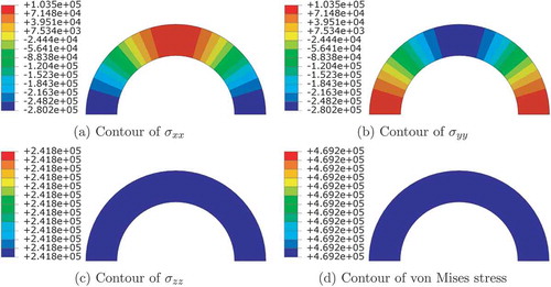
As derived in Section 2.1, the radial, circumferential and axial strains are constants in the cross-section, therefore the stress components should also be constants. Figure 5 is plotted in Cartesian coordinate system using coordinate projection, ${\sigma }_{xx}$ and ${\sigma }_{yy}$ change circumferentially but remain symmetrical about both $x$ and $y$ axes. On the other hand, ${\sigma }_{zz}$ ($z$ is the longitudinal direction) and von Mises stress remain constants on the $x-y$ plane cross-section.

The von Mises distribution at the end of each step for Case 2, step 1: residual stress, step 2: upon stent deployment representing mechanical loading, and step 3: upon growth, are shown in Figure 6, respectively.

Figure 6. Von Mises stress (Pa) distribution at different stages.

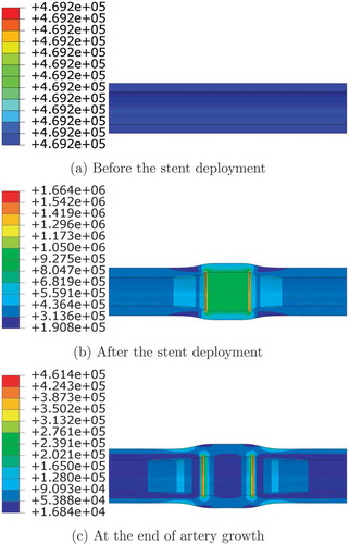
As shown in Figure 6, the stress distribution is changed by the tissue growth: before stenting takes place, the stress is uniform and low, it then becomes much higher and stress concentration is observed after the stent is deployed. Upon the growth, stress becomes more uniform showing the growth ameliorates the concentration significantly where only both ends of the loading area remain relatively higher stress. This change in stress distribution agrees with previous computational results observed in [10, 25].

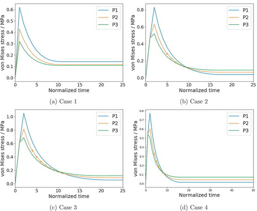
To study the impact of the residual stress on the restenosis quantitatively, we trace the von Mises stress at 3 different points in the middle cross-section of the vessel, along an arbitrary radius (the model is axisymmetric). To show the trend of von Mises stress in the radial direction, these points are chosen at the inner wall, the midpoint between inner and outer walls, and the outer wall, denoted as P1, P2, and P3, respectively, labeled in Figure 4.

The first observation of Figure 7 is that convergence is reached in all the cases. The restenosis process stops after approximately $20$ normalized time steps. Furthermore, at the initial step, the stress at the inner wall is the highest and that at the outer wall is the lowest. This appears for all cases. Without residual stress (as in Case 1), the value of the von Mises stress decreases with time but the relative relationship does not change. On the contrary, with residual stress (Cases 2 and 3), the von Mises stress at the inner wall decreases faster than the outer wall and becomes even lower than the outer wall in the end. This is because a higher stress concentration level leads to a higher growth rate, which is reflected in our model as Equation 16a, where the growth criterion function increases with the trace of Mandel stress. For the same reason, the average value of von Mises stress with the residual stress is smaller than that without residual stress. Interestingly, Case 4 has similar distribution as well as value of von Mises stress as Case 2, although it has larger axial strain. This indicates that axial stretching does not affect stress concentration.

Figure 7. Evolution of von Mises stress at the inner wall (P1), middle wall (P2), and outer wall (P3) .

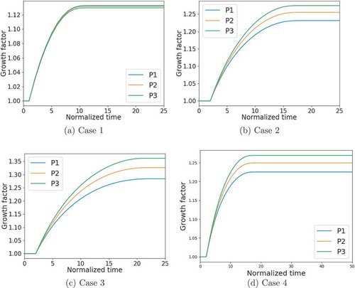
As a measure of the significance of the growth, the growth factors at these three points are plotted in Figure 8. Similarly, the residual stress changes the distribution pattern of growth factor, the outer wall has larger growth factor with the influence of the residual stress. The growth factor does not reach the upper limit of ${\theta }_g^{\mathrm{m}\mathrm{a}\mathrm{x}}=1.5$ in all four cases, but the maximum growth value increases corresponding based on increasing residual stress (from Case 1 to Case 3). The result shows that the larger the open angle or the residual stress, the more the vessel grows. As expected, due to the similar distribution of stress concentration, the growth factor profile of Case 4 is similar to that of Case 2.

Figure 8. Evolution of growth factor during growth at the inner wall (P1), middle wall (P2), and outer wall (P3) .

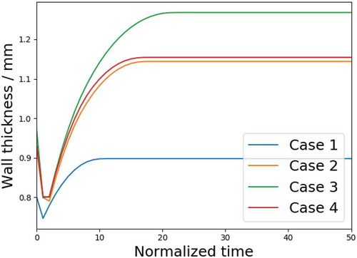
One important feature of the in-stent restenosis is the wall thickening, as reported in [22–24]. Figure 9 shows the change of the wall thickness in all cases. The wall thickness in Case 1 first decreases because of the expansion, then increases due to the growth. In Cases 2, 3 and 4, the arteries first undergo a ‘closing open angle’ process, which sets their wall thickness to the initial value of Case 1, then decrease further due to the expansion, and finally increase again due to growth. Even though wall thickening is observed in all cases, it is clearly most significant in Case 3, followed by Case 4, Case 2 and Case 1. This indicates the residual stress acts as an additional source of growth besides external loading such as stenting. The difference in the final thicknesses between Cases 2 and Case 4 is insignificant, but that of Case 2 and Case 3 differ by more than $10\mathrm{\%}$, which suggests that the growth is not only affected by the existence of the residual stress, but sensitive to the value of it.

Figure 9. Wall thickness during stent deployment and in-stent restenosis.

5. Conclusions

In this study, finite element simulations of the vessel tissue remodeling with varying degrees of residual stress are carried out with stress-modulated growth model. The volumetric growth process is captured, the wall thickening is observed, and it is found that the volumetric growth of the artery wall tends to even out lower the overall stress and the stress concentration. The residual stress is shown to have significant impact on the result of artery tissue growth: the residual stress results in greater stress and growth factor on the outer wall, which is opposite to the case without the residual stress. The wall thickening also increases with increasing residual stress. However, because the growth does not reach the upper limit, the stress concentration is ameliorated in all cases, thus the average von Mises stress at the final equilibrium state does not change significantly. The tissue wall growth or remodeling agrees qualitatively with existing numerical simulations and clinical observations. But the stress distribution is different from existing numerical results as the residual stress were not accounted for previously. In conclusion, based on the coupled model framework, the results show the residual stress has an significant effect on mechanical-driven tissue growth, therefore should be considered in tissue growth modeling.

Acknowledgments

Author Lucy T. Zhang would like to thank NSFC 11550110185, NSFC 11650410650, and NIH-2R01DC005642-10A1 for funding support.

Disclosure statement

No potential conflict of interest was reported by the authors.

Additional information

Funding

This work was supported by the Foundation for the National Institutes of Health [NIH-2R01DC005642-10A1];National Natural Science Foundation of China [11550110185,11650410650].

References

- Y.C. Fung, What are the residual stresses doing in our blood vessels? Ann. Biomed. Eng. 19 (3) (1991), pp. 237–249. doi:10.1007/BF02584301.
- D.P. Richman, R.M. Stewart, J.W. Hutchinson, and V.S. Caviness, Mechanical model of brain convolutional development, Science 189 (4196) (1975), pp. 18–21. doi:10.1126/science.1135626.
- T. Stylianopoulos, J.D. Martin, V.P. Chauhan, S.R. Jain, B. Diop-Frimpong, N. Bardeesy, B.L. Smith, C.R. Ferrone, F.J. Hornicek, and Y. Boucher, Others, Causes, consequences, and remedies for growth-induced solid stress in murine and human tumors, Proc. Natl. Acad. Sci. 109 (38) (2012), pp. 15101–15108. doi:10.1073/pnas.1213353109.
- L. Cardamone, A. Valentin, J.F. Eberth, and J.D. Humphrey, Origin of axial prestretch and residual stress in arteries, Biomech. Model. Mechanobiol. 8 (6) (2009), pp. 431–446. doi:10.1007/s10237-008-0146-x.
- T. Olsson and A. Klarbring, Residual stresses in soft tissue as a consequence of growth and remodeling: Application to an arterial geometry, Eur. J. Mechanics A/Solids 27 (6) (2008), pp. 959–974. doi:10.1016/j.euromechsol.2007.12.006.
- L.A. Taber and J.D. Humphrey, Stress-modulated growth, residual stress, and vascular heterogeneity, J. Biomech. Eng. 123 (6) (2001), pp. 528–535. doi:10.1115/1.1412451.
- E. Kuhl, Growing matter: A review of growth in living systems, J. Mech. Behav. Biomed. Mater. 29 (2014), pp. 529–543. doi:10.1016/j.jmbbm.2013.10.009.
- A.M. Zöllner, A.B. Tepole, A.K. Gosain, and E. Kuhl, Growing skin: Tissue expansion in pediatric forehead reconstruction, Biomech. Model. Mechanobiol. 11 (6) (2012), pp. 855–867. doi:10.1007/s10237-011-0357-4.
- G. Himpel, E. Kuhl, A. Menzel, and P. Steinmann, Computational modelling of isotropic multiplicative growth, CMES Comput. Modeling Eng. Sci. 8 (2005), pp. 119–134.
- E. Kuhl, R. Maas, G. Himpel, and A. Menzel, Computational modeling of arterial wall growth: Attempts towards patient-specific simulations based on computer tomography, Biomech. Model. Mechanobiol. 6 (5) (2007), pp. 321–331. doi:10.1007/s10237-006-0062-x.
- G.D. Dangas, B.E. Claessen, A. Caixeta, E.A. Sanidas, G.S. Mintz, and R. Mehran, In-stent restenosis in the drug-eluting stent era, J. Am. Coll. Cardiol. 56 (23) (2010), pp. 1897–1907. doi:10.1016/j.jacc.2010.07.028.
- D.M. Pierce, T.E. Fastl, B. Rodriguez-Vila, P. Verbrugghe, I. Fourneau, G. Maleux, P. Herijgers, E.J. Gomez, and G.A. Holzapfel, A method for incorporating three-dimensional residual stretches/stresses into patient-specific finite element simulations of arteries, J. Mech. Behav. Biomed. Mater. 47 (2015), pp. 147–164. doi:10.1016/j.jmbbm.2015.03.024.
- T.J. Van Dyke and A. Hoger, A new method for predicting the opening angle for soft tissues, J. Biomech. Eng. 124 (4) (2002), pp. 347. doi:10.1115/1.1487881.
- A. Klarbring, T. Olsson, and J. Stålhand, Theory of residual stresses with application to an arterial geometry, Arch. Mechanics 59 (2007), pp. 341–364.
- A. Menzel, A fibre reorientation model for orthotropic multiplicative growth, Biomech. Model. Mechanobiol. 6 (5) (2007), pp. 303–320. doi:10.1007/s10237-006-0061-y.
- E.K. Rodriguez, A. Hoger, and A.D. McCulloch, Stress-dependent finite-growth in soft elastic tissues, J. Biomech. 27 (4) (1994), pp. 455–467. doi:10.1016/0021-9290(94)90021-3.
- A. Goriely and M. Ben Amar, On the definition and modeling of incremental, cumulative, and continuous growth laws in morphoelasticity, Biomech. Model. Mechanobiol. 6 (5) (2007), pp. 289–296. doi:10.1007/s10237-006-0065-7.
- S. Göktepe, O.J. Abilez, and E. Kuhl, A generic approach towards finite growth with examples of athlete’s heart, cardiac dilation, and cardiac wall thickening, J. Mech. Phys. Solids. 58 (10) (2010), pp. 1661–1680. doi:10.1016/j.jmps.2010.07.003.
- E. Kuhl, A. Menzel, and P. Steinmann, Computational modeling of growth, Comput. Mech. 32 (1–2) (2003), pp. 71–88. doi:10.1007/s00466-003-0463-y.
- J. Cheng and L.T. Zhang, A general approach to derive stress and elasticity tensors for hyperelastic isotropic and anisotropic biomaterials, Int. J. Computational Met. 15 (1) (2017), pp. 1850028. doi:10.1142/S0219876218500287.
- G. Holzapfel, Nonlinear Solid Mechanics: A Continuum Approach for Engineering, First Edit, Wiley, 2000.
- J.J. Wentzel, R. Krams, J.C.H. Schuurbiers, J.A. Oomen, J. Kloet, W.J. van der Giessen, P.W. Serruys, and C.J. Slager, Relationship between neointimal thickness and shear stress after Wallstent implantation in human coronary arteries, Circulation 103 (13) (2001), pp. 1740–1745. doi:10.1161/01.CIR.103.13.1740.
- P.H. Stone, A.U. Coskun, S. Kinlay, M.E. Clark, M. Sonka, A. Wahle, O.J. Ilegbusi, Y. Yeghiazarians, J.J. Popma, and J. Orav, Others, Effect of endothelial shear stress on the progression of coronary artery disease, vascular remodeling, and in-stent restenosis in humans, Circulation 108 (4) (2003), pp. 438–444. doi:10.1161/01.CIR.0000080882.35274.AD.
- K.C. Koskinas, Y.S. Chatzizisis, A.P. Antoniadis, and G.D. Giannoglou, Role of endothelial shear stress in stent restenosis and thrombosis, J. Am. Coll. Cardiol. 59 (15) (2012), pp. 1337–1349. doi:10.1016/j.jacc.2011.10.903.
- V. Alastrué, M.A. Martínez, and M. Doblaré, Modelling adaptative volumetric finite growth in patient-specific residually stressed arteries, J. Biomech. 41 (8) (2008), pp. 1773–1781. doi:10.1016/j.jbiomech.2008.02.036.
- P. Ciarletta, M. Destrade, and A.L. Gower, On residual stresses and homeostasis: An elastic theory of functional adaptation in living matter, Sci. Rep. 6 (March) (2016), pp. 1–8. doi:10.1038/srep24390.
- J. Ohayon, O. Dubreuil, P. Tracqui, H.S. Le Floc’, G. Rioufol, L. Chalabreysse, F. Thivolet, R.I. Pettigrew, and G. Finet, Influence of residual stress/strain on the biomechanical stability of vulnerable coronary plaques: Potential impact for evaluating the risk of plaque rupture, Am. J. Physiol. Heart Circ. Physiol. 293 (3) (2007), pp. 1987–1996. doi:10.1152/ajpheart.00018.2007.
- L. Tian, S.R. Lammers, P.H. Kao, J.A. Albietz, K.R. Stenmark, H.J. Qi, R. Shandas, and K.S. Hunter, Impact of residual stretch and remodeling on collagen engagement in healthy and pulmonary hypertensive calf pulmonary arteries at physiological pressures, Ann. Biomed. Eng. 40 (7) (2012), pp. 1419–1433. doi:10.1007/s10439-012-0509-4.