
 ?Mathematical formulae have been encoded as MathML and are displayed in this HTML version using MathJax in order to improve their display. Uncheck the box to turn MathJax off. This feature requires Javascript. Click on a formula to zoom.
ABSTRACT
As an ideal high-density storage unit, magnetic nanorings have become a research hotspot in recent years. We can both study the evolution of microscopic state of magnetization and acquire macroscopic magnetic properties by micromagnetic simulation, which has thus been widely used. However, traditional micromagnetism cannot simulate complex stress state. Due to the introduction of microelasticity theory, the phase field method for magnetic materials can be used to calculate the coupling effect of stress and magnetic field. However, the computing model usually needs to satisfy periodic boundary condition. In this paper, the phase field simulation combined with the finite element method is employed. By using user defined element, the evolution of magnetic domain structures of the double-hole nanorings has been studied. In different diameter of the holes and external magnetic field direction, we have found seven kinds of magnetic domain evolution mechanism. Among them, the twin-vortex evolution mechanism with high stability and low demagnetization interference characteristics of advantages, has good application prospect in magnetic random-access memory (MRAM) unit.
Graphical Abstract

Introduction
In recent years, magnetic random memory (MRAM) based on GMR (or TMR) effect has attracted great interest from researchers in various countries because of its nonvolatile, high density and high-speed reading. As an ideal high-density storage unit, magnetic nanorings have become the focus of research in recent years. In 2000, J G, Zheng Y, Prinz G A [Citation1] proposed a random-access memory VMRAM design based on micromagnetic simulation analysis, which utilizes the macromagnetic resistance effect of vertical magnetic multi-layer, has good robustness by making the storage unit into a circular magnetic multi-layer stack, and estimates the limit storage surface density of 400Gbits/in2. In 2001, Schneider M, Hoffmann H, Zweck J [Citation2] prepared a sub-micron Pomo alloy disc using electron beam lithography and liftoff techniques, observed the magnetization flip mechanism and remaining magnetic configuration using the Lorenz transmission electron microscope, and revealed the possibility of adjusting the magnetization spin by introducing slight geometric asymmetry. In 2001, Rothman J, Kläui M, Lopez-Diaz L, et al [Citation3]. studied the evolution of Co(100) magnetic ring magnetism using magnetic measurements and micromagnetic simulations, and discovered a new stable double domain state, the onion state. In 2002 Lai, Mei-Feng et al [Citation4]. simulated the soft magnetic material Pomo alloy nanoring with micromagnetic, discovered a new stable twin-vortex state, and compared it with magnetic force microscope (MFM) images. In 2005, Moore T A, Hayward T J, Tse D H Y, et al [Citation5]. used magneto-optical Kerr effect (MOKE) magnetic forces to determine the hysteresis return of the polycrystalline Permalloy ring with an outer diameter 2 μm and 5 μm, and used micromagnetic simulations to reveal the onion-to-vortex flipping mechanism, pointing out that the positive and reverse flipping of the vortex state is random, depending on historical configuration and thermal fluctuations. In 2005 M. Rahm et al [Citation6]. found that by introducing hole defects, they could increase the number of hysteresis loops. They then investigated multiple holes and applied magnetic field control to make the magnetic domain state switch between multiple steady states, which they wanted to achieve multi-process storage. Furthermore, they designed a logical memory because their magnetic field flips do not need to be applied to saturation, and their flip fields are much smaller. In addition, they studied magnetic field flip fields and logical states. In 2006, Zhu F Q, Chern G W, Tchernyshyov O et al [Citation7]. prepared asymmetric nanorings to regulate the vortex formation process by changing the direction of the external magnetic field. In 2006 Mani A S, Geerpuram D, Baskaran V S et al [Citation8]. studied the effects of shape on vortex formation and vortex chirality, and found that the introduction of asymmetrically provided an accurate control of the flip mechanism. In 2007, Yang T, Hara M, Hirohata A et al [Citation9]. prepared Co nanorings of horizontal size of deep sub-microns, and experiments revealed that the giant magneto-resistance effect of vertical ring planes can effectively describe a very small magnetic nanoring, and found that the transition between the nanoring onion state and the vortex state can be achieved not only by applying an external magnetic field but also by vertically through direct current. In 2012, Huang C H, Cheng N J, Wu F S et al [Citation10]. used micromagnetic software to simulate asymmetric Pomo alloy rings, demonstrating that asymmetric rings can regulate not only the vortex chirality but also the vortex formation and vanish field.
With the improvement of computer storage and computation speed, micromagnetic simulation method has been developed rapidly and widely used. The main calculation methods can be divided into two broad categories, namely, the finite differential method(FDM) proposed by Hughes [Citation11] in 1983, and the finite element method(FEM) proposed by Fredkin and Koehler [Citation12] in 1987. Since the demagation field is along-range interaction field and its calculation are time-consuming, Bertram and Zhu [Citation13] propose to introduce a fast Fourier transformation (FFT) in FDM calculations to calculate the demagation field. Magnetic scalcation potentials ϕ are usually introduced in finite element simulations to calculate static magnetic fields. Because the boundary of the magnetic field is an open Dirichilet boundary condition, the magnetic extraterritorial infinite area can be mapped to a finite area by angle-protected transformations [Citation14], but these transformations typically apply only to the boundaries of a particular shape. Since the regression field decays rapidly in the air, the demagation magnetic field can also be approximated by taking the outer region large enough to approximate the de-magnetic field [Citation15], but this will increase the amount of storage and calculation. Fredkin [Citation16] proposed in 1990 to combine FEM with boundary integrals to calculate the demagation magnetic field, which greatly improved the computational efficiency and gradually developed the FEM-BEM (Boundary Element Method) hybrid calculation method.
Phase-field simulation methods were developed in the 1970s, initially to bypass the difficulty of tracking solid–liquid interfaces when simulating solidified tissue, and were later widely used in various tissue evolution problems. The phase field model describes different phases by introducing continuously changing field variables – order parameters in the entire calculation area. The order parameters change sharply at the interface, and there is no need to track the geometry of the interface. Therefore, the phase field is a diffuse interface model. The phase field theory is based on statistical physics. According to the Ginzburg-Laudau phase transition theory, it reflects the combined effects of diffusion, ordering potential and thermodynamic driving force through differential equations. As a powerful computational simulation method, phase field method is widely used in the simulation and prediction of material-based morphology and microstructive evolution [Citation17]. In recent years, this method has been used to study the micro-evolution and macro-performance of ferromagnetic, ferroelectric and magnetic composite materials. In 2003, Koyama [Citation18] used the phase field method to study the microstructure evolution of ferromagnetic shape memory alloys (MSMAs) Ni2MnGa under applied stress and magnetic field. Its free energy includes chemical-free energy, gradient energy, elastic energy, and magnetic energy. Among them, the magnetic energy only considers anisotropic properties. In 2012, Miehe [Citation15] used node displacement, magnetic potential, and magnetization vector as field variables, established corresponding finite element equations based on elastic mechanics, magnetostatic theory and TDGL evolution equations, compiled 2D magnetic elements, and analyzed the regulation of the magnetic field and stress on the micro/nano structure of permalloy. When solving the demagnetization problem, Miehe takes a large enough external free space, and assume that the magnetic potential at the boundary decays to zero. Without considering the air element, Wang [Citation19] in 2013 established a 3D model and analyzed the regulation of the nano-magnetic structure by strain, magnetic field and their coupling effects. Using this method can not only calculate the boundary of complex shapes, but also calculate the force-magnetic coupling response of materials under complex stress. However, this method is not yet mature enough and needs to be further developed and improved.
In this paper, the method of combining finite element and phase field [Citation20] is used to derive the corresponding incremental variational principle from the equations of mechanics, magnetostatics and magnetization vector motion. The finite element equation is established, and the two-dimensional is compiled through the ABAQUS software subroutine development module. The ferromagnetic element can simulate the microstructure of any boundary under the action of magnetic field and complex stress field. Through the written user element, we study the evolution mechanism of the magnetic domain of the double-hole nanoring, and focus on the regulation mechanism of the geometric aperture and the direction of the external magnetic field to the double-hole ferromagnetic nanoring magnetic domain. Under the parameters of different geometric aperture and external magnetic field direction, we found seven kinds of magnetic domain evolution paths: twin-vortex mechanism, left and right vortex mechanism, ‘S’ evolution mechanism, ‘S’ + ‘C’ mechanism, ‘S’ and ‘twin-vortex mechanism’, ‘S’ + left vortex mechanism, left vortex mechanism. Among them, the twin-vortex mechanism has a good application prospect in random storage unit because of its advantages of high stability and low demagnetic interference.
Phase field model and finite element formulation
Basic equations and boundary conditions
Mechanical equation
Under the linear elasticity and small deformation hypothesizes, the basic equation of elasticity can be used to describe the behavior of magnetic materials. The mechanical equilibrium equation can be expressed as:
represents stress and
represents elastomer.
is the second derivative of
with respect of time
. Since the body force
is not considered in this problem, and the effect of inertial force
is very small, which can be ignored, formula (1) can be simplified as [Citation15]
Boundary conditions can be represented as [Citation15]
represents the magnetic elastomer boundary,
represents the surface force on the boundary, and
represents the direction vector of the common line outside the boundary. Geometric equations based on the assumption of small deformation can be represented [Citation15]
where represents strain,
represents displacement,
. By (2)-(4) one can get the displacement variational equation of elasticity:
Magnetostatics equation
The total magnetic field can be decoupled into two parts, the de-magnetic field and the external magnetic field, recorded as [Citation20]
represents the total magnetic field,
represents the de-magnetic field, is determined by the geometry of the structure and the magnetization state, and
represents the external magnetic field. Degenerate Maxwell equations can get magnetostatic Equationequations [19
(19)
(19) ]
Among them is magnetic induction strength, which can be expressed as the relationship between it and the magnetic field [Citation20]
The saturation magnetization strength represents the magnitude of the magnetization vector
, which is the material constant and represents the direction cosine of the magnetization vector. When the external magnetic field
is uniform,
The relationship between the magnum potential and the demagnetic field can be expressed [Citation20]
Boundary conditions at the magnetic material interface can be represented
where ,
represents the magnetic potential of the magnetic body and the outer boundary, respectively. The first formulation in (11) indicates that the magnetic potential is continuous at the magnetic body boundary, and the condition is automatically satisfied because it is a field function in finite element simulation. The second means that the flux flowing in and out of the boundary is equal, i.e., the static flux is 0. Magnetic potential needs to be satisfied in infinity
Because the de-magnetic field decays rapidly in the air, a large enough area can be taken outside the magnet to make the magnetic potential at the boundary of the region 0, thus replacing infinity boundary conditions (12) with an approximate boundary condition [Citation15]
is the boundary of the external air area. According to (9)-(11) and (13) the magnetostatic variational equation can be derived
where the air magnetizes the vector .
Motion equations of magnetization vector
The motion equation of the magnetization vector usually adopts the LLG equation, but for the study of static magnetic properties, the TDGL equation can also be used [Citation19]
whereis the motion coefficient,
is the density of free energy, and [Citation15]
The density of free energy in the magnetic body can be expressed as follows:
where is the Anisotropy energy,
is the exchange energy,
is the elastic energy,
is the sum of the magnetostatic energy and the external magnetic energy, and
is the constraint term, which is called the penalty function in the finite element method. The specific forms of each item will be given below. For cubic anisotropic crystal, its magnetocrystalline anisotropy can be expressed as [Citation19]
where ,
are material constant, respectively. The exchange energy is related to the change gradient of the magnetization intensity and can be represented as follows [Citation19]:
where is the exchange constant. Elastic energy expressions can be divided into two parts:
represents energy items related only to elastic deformation, and
energy items related to magnetic elastic coupling, as follows [Citation19]:
where ,
,
and are the anisotropic elastic constants of cubic crystals,
and
are the magnetostriction coefficients. For an ideal crystal of cubic crystal system, its elastic properties are completely described by a matrix of elastic constants (stiffness coefficient)
, which contains three independent elastic constants
,
, and
. Among them, only the constant
has a direct physical meaning as a measure of the resistance of the crystal to the shear force in the <100> cube plane along any direction lying in this plane. The matrix coefficients
and
have no such simple explanation. Only by using the corresponding Hooke’s law symbols can we understand their meaning [Citation21]. For cubic materials, there are two independent magnetostriction constants
and
. And
,
are the saturation magnetostrictions along the <100> and <111> axes of the crystal [Citation22]. And
where is the vacuum magnetic conductivity. Magnetization vectors should meet constraints
, which are constrained by the introduction of energy terms
whose expressions can be written as [Citation19]
This term is equivalent to the penalty function term in the finite element method. The value of is not the larger the better, too large will easily cause singularity and cause the calculation to fail to converge. It should be determined according to the specific situation. Without considering the surface anisotropy, the magnetization vector usually satisfies the following equation at the boundary [Citation20]:
Regarding the variation of the free energy density to the magnetization vector
, there is the following relationship [Citation15]:
According to (15), (25), (26), we can get
The basic equations and boundary conditions related to mechanics, magnetostatics, and magnetization vector motion are given above, which are the basis for deriving the finite element form.
Phase field finite element form
The weak form of equivalent integrals
Since there is a demagnetizing field in the air element, its free energy density can be expressed as
Then according to the free energy density (17) in the ferromagnetic body, the total-free energy within the model can be obtained [Citation20]:
External forces can be expressed as:
The dissipation potential of the magnetization vector motion is introduced [Citation15]:
where is the inverted number of the motion coefficient. In a time step
, set the interval to
, and the total potential energy of the system can be written as [Citation15]
where,
represent the free energy of the moment
and the external force work, which are constants, so that let the constant
. There are also the following relationships
is the cosine of the magnetization vector direction at time
. (32) can be rewritten as [Citation20]
From the potential energy functional form in (34), the differential Equationequations (2)(2)
(2) , (Equation9
(9)
(9) ), (Equation15
(15)
(15) ) and boundary conditions (3), (11), (25) can be derived. Among them, there is a relationship
Therefore, the total potential energy given in (34) corresponds to these basic equations and boundary conditions. The condition for the extreme value of the functional is
This results in a weak form of equivalent integral for the problem:
In addition, it is easy to obtain the equivalent integral weak form in (37) by properly processing and adding the variational forms of (5), (14), (27).
Finite element equation
In this work, a multi-field coupled finite element was developed via the ABAQUS user subroutine module. In order to establish the finite element equation, the field variable of the node is first determined, that is, the general displacement variable is as follows [Citation20]:
The field variables of the magnetic element include displacement, the magnetic scale potential, and the magnetization direction vector, and the field variables of the air element contain only the magnetic scale potential. The general strain corresponding to the general displacement can be represented [Citation20]
general stress can be expressed as
The element node displacement matrix can be represented [Citation20]
where is the number of element nodes. The generalized displacement field variables can be obtained by interpolating the nodes [Citation20]
The expression that can be generally strained is obtained accordingly [Citation20]
Based on the above definition, the equivalent integral weak form (37) can be rewrite into the following matrix form [Citation20]:
Suppose , where
is the overall nodal displacement matrix, then (44) can be rewritten as [Citation20],
which is the residual equation of the coupled problem and can be solved by the Newton iteration method [Citation20]:
The label represents the
th iteration step. The above formula can be written as [Citation20]
where [Citation20]
is the tangent stiffness matrix. Thus, the form of the element residual matrix and the stiffness matrix can be obtained [Citation20]:
Through the residual and stiffness matrix of each element, the overall stiffness matrix and nodal load array are assembled, and the nodal value at the next time step can be obtained by iterative solution in one time step. Through time integration, iterative solution for the next time step is performed until the system reaches a stable equilibrium state.
Specific form of 2D element
In this paper, the 2D triangle element is used, and the magnetic element adopts the Hammer integral of four integral points, whose general displacement and general strain can be written as follows [Citation20]:
The element node displacement matrix can be represented
The relationship between general displacement, general strain and node variables is [Citation20]
Among them,
The general stress matrix corresponding to the general strain can be represented
The specific expression is shown in (). For a cubic magnetostrictive material, the deformation associated with the local magnetization is described by the stress–free strain [Citation23]. Thus, for the 2D condition we assume for the description of stress-free strain. The generalized shear modulus matrix
is defined by
, and the specific form is shown in (). Since
is a symmetric matrix, only the upper triangular part of the expression is written here, and the unspecified terms are all zero.
Table 1. Concrete expression of 2D magnetic element S matrix
Table 2. 2D magnetic element D matrix upper triangular expression
For the air element outside the ferromagnetic body, the corresponding general displacement, generalized strain, and generalized stress matrix can be represented
Its node displacement matrix and matrix
are
The tangent stiffness matrix can be represented
The magnetic potential remains continuous on the interface between the magnetic element and the air element, on the outer boundary of the air element
. Only the magnetic potential is used as a variable for the magnetic field of the air element. By coupling the magnetic element to the air node on the boundary, the potential is continuous. In the simulation process, the backward Euler method is used for time integration.
Magnetic domain evolution mechanism of double-hole ferromagnetic nanorings
Through the written user 2D element in ABAQUS software, the magnetic domain evolution mechanism of the double-hole nanoring under a magnetic field is studied, the evolution mechanism of the magnetic domain of the double-hole ferromagnetic nanoring with the geometric aperture and the direction of the external magnetic field is analyzed, and its application prospect on random storage units is explored.
Simulation model and parameter settings
The two-hole ferromagnetic nanoring calculation model is shown in . The magnetic easy axes are along x-axis directions. Where the outer diameter of the nanoring is D = 0.1 μm, the two round holes are symmetrical to the left and right, both in diameter d = 0.025 μm, and the center distance is 0.05 μm. The direction of uniform magnetic field application and the angle of y-axis direction are recorded, the hysteresis return line in different hole aperture and direction of different external magnetic field is calculated, and the evolution of magnetization state is examined. The calculation parameters of the nanorings are based on the FeGa material parameters [Citation23] with the Zener anisotropy factor [Citation24,Citation25], as () shows. The thickness of the simulated magnet has strong influence on the micromagnetic structure especially in the thin film. However, we consider it that since the magnetic easy axes of FeGa material are along <100> directions [Citation23], we performed the simulations in essentially 2D systems. There are several researches obey the rules in computing in 2D simulations. In 2D simulations, the field parameters in the z-axis consider to be uniform, which contains no information of the thickness. The further effects of thickness could be discussed in our future work.
Figure 1. Schematic diagram of calculation model of symmetric double-hole nanoring
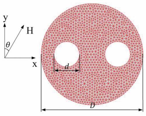
Table 3. Material parameters (FeGa) [Citation23] for the simulation
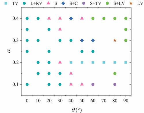
The revolution mechanism of the geometric aperture and the direction of the external magnetic field on the magnetic domain of the double-hole ferromagnetic nanoring
By defining the aperture ratio:
changing the geometric aperture ratio of the ring and the angle of the external magnetic field
, through static cyclic loading by magnetic field, we calculate the hysteresis return line under different regulatory parameters, and observe the evolution of the magnetic field. The magnetization direction is randomly oriented in the initial calculation. () shows a summary diagram of the evolution mechanism of symmetrical double-hole ferromagnetic nanorings. The horizontal coordinates in the figure are the angle between the direction of the applied magnetic field and the direction of the
axis, and the ordinate is the aperture ratio
. In the calculation parameter grid of aperture ratio
from 0.10 to 0.40 with range interval 0.05, applied external magnetic field angle
from 0° to 90° with range interval 10°, we found a total of 7 evolutionary mechanisms, namely: twin-vortex mechanism, left and right vortex mechanism, ‘S’ evolution mechanism, ‘S’ + ‘C’ mechanism, ‘S’ + twin-vortex mechanism, ‘S’ + left vortex mechanism, and single left vortex mechanism.
Figure 2. Summary of the evolution mechanism of the symmetric double-hole ferromagnetic nanoring (TV: twin-vortex mechanism, L+ RV: left and right vortex mechanism, S: ‘S’ evolution mechanism, S + C: ‘S’ + ‘C’ mechanism, S+ TV: ‘S’ + twin-vortex mechanism, S+ LV: ‘S’ and left vortex mechanism, and LV: left vortex mechanism)
Twin-vortex mechanism
We found a new stable vortex state in the regulatory parameters: aperture ratio , applied external magnetic field angle
from 40° to 90° range, twin-vortex state (TV), as shown in (). The twin-vortex magnetic domain structure is similar to but different from the vortex closed domain structure of a single-hole ring: the same vortex-closed domain structure as the single-hole ring with a small demagnetizing field; the vortex domain structure of the single-hole ring surrounds the hole to form a stable vortex domain structure, but the double-hole ring twin-vortex domain structure surrounds the two holes to form two vortex domain structures with opposite rotation directions.
Figure 3. Twin-vortex magnetization state diagram
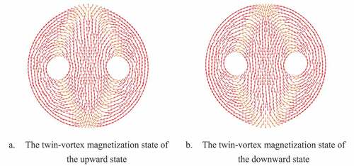
For twin-vortex magnetization state, Nipun A [Citation26] in 2007 demonstrated twin-vortex in 30-nm-thick Co nanopatterned double pac-man (DPM) elements (with Outer Diameter (OD): 400 nm, notch radius: 120 nm, and Slot Angle 60°), fabricated by electron-beam lithography (EBL) and liftoff processing, when the field is applied in an orthogonal direction, using Lorentz microscopy and off-axis electron holography.
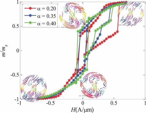
() shows the hysteresis loop of the twin-vortex evolution mechanism. The horizontal coordinates in the figure are the size of the external magnetic field , and the ordinates are the ratio of the size of the magnetization vector
to the intensity of the saturation magnetization
. The external magnetic field of the double-hole ring is greater than the strength of the positive saturated magnetic field and less than the strength of the reverse saturation magnetic field is in the onion state (ON), when the magnetic field decreases the magnetization state of the ring evolves from the onion state to the twin-vortex state (TV), i.e., there is an ON-TV mechanism, similar to the onion state (ON) – vortex state (VT) mechanism of the single-hole ring. Due to the closure of the twin-vortex magnetic field, when the external magnetic field is reduced to zero, the demagnetization field is very small, which retains the advantages of the closed single-hole ring vortex magnetic domain, so that the adjacent magnetic ring does not interfere with each other directly, which has great advantages for improving the density of the storage unit.
Figure 4. Twin-vortex mechanism hysteresis loop
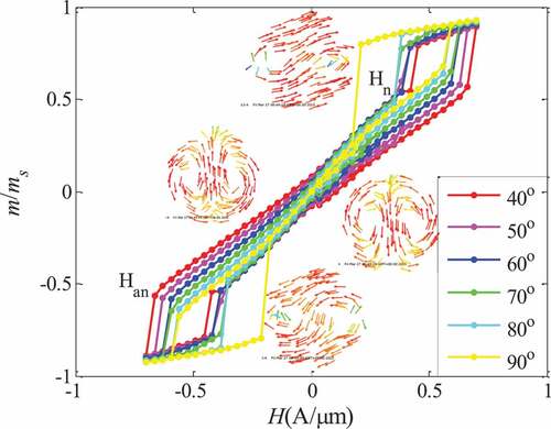
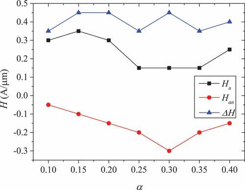
In this paper, the critical flip field of the onion state-vortex state is called the vortex-vortex nuclear field , and the critical flip field of the vortex-onion state is called the vortex vanishing field
, then
is the magnetic field range of the twin-vortex state, the size of which shows the stability of the twin vortex state under the change of the magnetic field: the larger , the more stable the twin-vortex state; vice versa.
Figure 5. Variation curve of ,
,
under different applied magnetic field angle
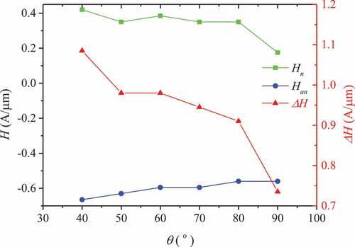
() shows the vortex nucleation field , vortex vanishing field
, and magnetic field range
in the twin-vortex state as a function of the applied magnetic field angle
. The vortex nuclear field
decreases with the increase of the magnetic field application angle
, the vortex vanishing field
increases with the increase of the magnetic field application angle
, and the magnetic field range
decreases with the increase of the applied magnetic field angle
. That is, the stability of the twin-vortex state decreases as the magnetic field application angle
increases.
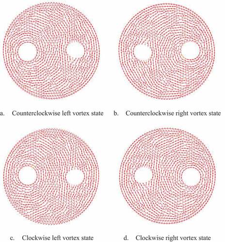
Figure 6. Left and right vortex magnetization state diagram
Left and right vortex mechanism
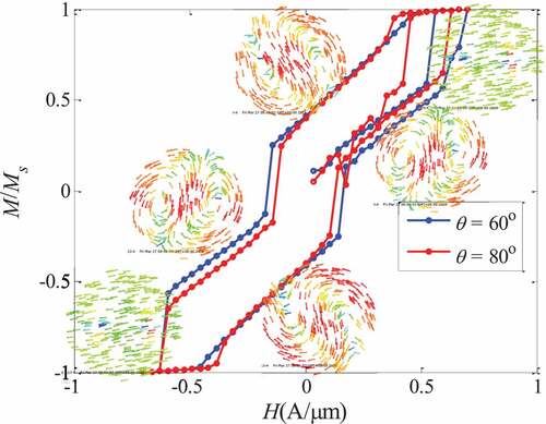
The control parameters of the left and right vortex have a relatively wide range of values: the aperture ratio range from 0.10 to 0.40, the angle of the applied external magnetic field θ from 0° to 60°, which is a relatively common evolutionary mechanism in the double-hole ring, as () shown.
The left and right vortex mechanism is: when the magnetic field is large, it is in a positive saturation state; when the magnetic field is reduced to a certain value, the magnetization state of ()) will appear, that is, the vortex structure surrounding the small ring on the left in a counterclockwise direction. At this time, there is a positive net magnetization; when the reverse magnetic field increases, a vortex structure surrounding the small ring on the right will appear as a whole counterclockwise, as shown in ()), at this time there is a reverse net magnetization; When the magnetic field increases to a certain value, the reverse saturation magnetization state will appear; when the reverse magnetic field decreases, the vortex structure surrounding the left small ring and the right small ring will appear in sequence, but the rotation direction is opposite, changing from counterclockwise It becomes clockwise, as shown in ()). The hysteresis loop diagram of the left and right vortex evolution mechanism is shown in (). We also mark the vortex nucleation field and the vortex vanishing field
, and observe the changes of the vortex nucleation field
, vortex vanishing field
, and magnetic field range
with the applied magnetic field angle
and aperture ratio
.
For Left and right vortex states, Rahm M [Citation27]. in 2004 demonstrated the existence of two metastable vortex states with the vortex center either pinned at the left or right antidot in disks consist of Permalloy, 30 nm thick, with a 10 nm protective Ti layer, with diameters of 500 nm, containing two antidots with center-to-center distances d of 150 and 200 nm, measured with micro-Hall magnetometry.
() shows the vortex nucleation field , vortex vanishing field
, and magnetic field range
in the left vortex state as a function of the applied magnetic field angle
. The vortex nucleation field
decreases with the increase of the magnetic field angle
, and the vortex vanishing field
also decreases with the increase of the magnetic field angle
. The magnetic field range
is not greatly affected by the change of the applied magnetic field angle
, that is, the stability of the left vortex state is not greatly affected by the change of the applied magnetic field angle
.
() shows the vortex nucleation field , vortex vanishing field
, and magnetic field range
in the left vortex state as a function of the geometric aperture ratio
. The vortex nucleation field
first decreases and then increases as the aperture ratio
increases. The vortex vanishing field
also decreases first and then increases with the aperture ratio
. The magnetic field range
is not greatly affected by the change in the geometric aperture ratio
, namely the stability of the left vortex state is not greatly affected by the change of the geometric aperture ratio
.
In short, the stability of the left vortex state is not affected by the change in the angle of the applied magnetic field and the ratio of geometric aperture
.
Figure 7. Hysteresis loop of left and right vortex evolution mechanism
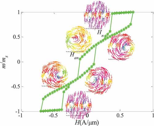
Figure 8. Variation curve of ,
,
under different applied magnetic field angle
(
)
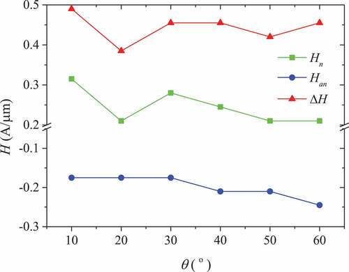
Figure 9. Variation curve of ,
,
under different aperture ratio
(
)
‘S’ evolutionary mechanism
The ‘S’ evolutionary mechanism regulates the distribution of parameters in small areas, only in cases where the aperture is quite large and relatively small (
), and the angle of the magnetic field
is applied.
Figure 10. ‘S’ state magnetization state diagram
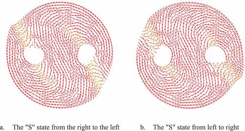
Figure 11. Hysteresis loop of ‘S’ evolution mechanism
The ‘S’ state evolution mechanism includes a new state of the double-hole ring: the ‘S’ state. The magnetization state of the ‘S’ state is that the two-hole ring contains two 180° domain walls, forming a magnetization vector from the right side of the right hole around the right hole to the middle and then around the left hole, and finally flowing out on the left side of the left hole (flowing from right to left, and vice versa from left to right), as shown in ().
() shows the hysteresis loop of ‘S’ evolution. When the forward magnetic field is unloaded, the magnetization state of the double-hole ring changes from the positive saturation state to the ‘S’ state flowing from right to left. When the magnetic field continues to unload and enters the reverse loading, the magnetization state of the double-hole ring turns from the ‘S’ state magnetization flowing from right to left to the ‘S’ state flowing from left to right, and the magnetization state of the reverse magnetic field continues to increase and it will enter the reverse saturation state.
The ‘S’ + ‘C’ mechanism
The ‘S’ + ‘C’ evolution mechanism has a relatively small regulatory parameter area, which appears when the aperture ratio is relatively large (
) and the applied magnetic field angle
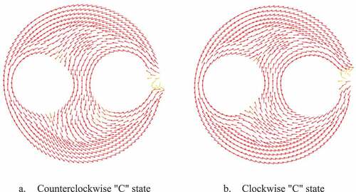
. The evolution path of the ‘S’ + ‘C’ mechanism consists of the ‘S’ state and the ‘C’ state. The magnetization state of the ‘C’ state is shown in ().
Figure 12. ‘C’ state magnetization state diagram
For ‘S’ and ‘C’ states, Jonathan K H [Citation28] in 2003 simulated permalloy disks and observed in-plane magnetization buckle states, including first-order buckle state, C state, observed in a diameter of 200 nm and a diameter-to-thickness ratio d/t of 20 at 0-mT field, as well as second-order buckle state, S state, observed in a diameter of 500 nm and a diameter-to-thickness ratio d/t of 3 at 3-mT field.
() shows the ‘S’ + ‘C’ mechanism evolutionary hysteresis loop. When a large positive magnetic field is applied, the forward magnetization of the double-hole magnetic ring is saturated, and as the magnetic field decreases, it enters the ‘S’ flowing from right to left. When the magnetic field is reduced to zero and a reverse magnetic field is applied, the ‘S’ state does not flip and jumps to the counterclockwise ‘C’ state. The reverse magnetic field continues to increase, and the magnetic ring changes from the counterclockwise ‘C’ state to the reverse saturation state.
‘S’ + twin-vortex mechanism
The ‘S’ + twin-vortex mechanism only appears when the aperture ratio and the applied magnetic field angle
, 80°. () shows the hysteresis loop diagram of ‘S’ + twin-vortex mechanism. Like the ‘S’ + ‘C’ mechanism, when the positive magnetic field is large, the positive magnetization of the double-hole magnetic ring is saturated. As the magnetic field decreases, it enters the ‘S’ state flowing from right to left. When the reverse magnetic field is applied, the ‘S’ state does not turn over and jumps to the twin-vortex magnetization state of the upward state. The reverse magnetic field continues to increase. The magnetic ring enters the reverse saturation state from the twin-vortex magnetization state of the upward state.
Figure 13. ‘S’ + ‘C’ mechanism evolution hysteresis loop diagram ()
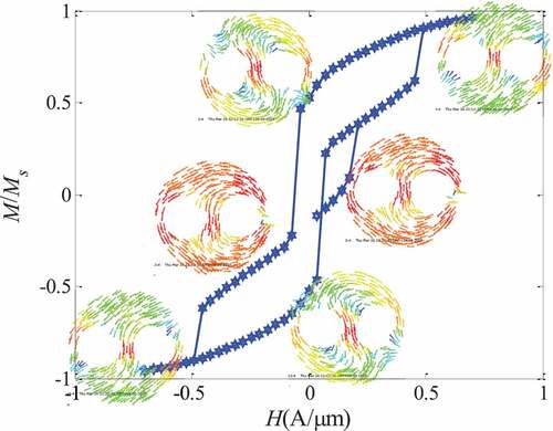
Figure 14. Hysteresis loop diagram of ‘S’ + twin-vortex mechanism (α = 0.10)
‘S’ + left vortex mechanism
The ‘S’ + left vortex mechanism appears when the aperture ratio α is larger or smaller, , and the applied magnetic field angle
. The hysteresis loop diagram of the ‘S’ + left vortex mechanism is shown in (). Like the ‘S’ + ‘C’ mechanism, when the positive magnetic field is large, the positive magnetization of the double-hole magnetic ring is saturated. As the magnetic field decreases, it enters the ‘S’ state that flows from right to left. When the magnetic field is reduced to zero and a reverse magnetic field is applied, the ‘S’ state does not flip and jumps to a counterclockwise left vortex state, and the reverse magnetic field continues to increase. The magnetic ring changes from a counterclockwise left vortex state to reverse saturation state.
Figure 15. ”S” + Left vortex mechanism hysteresis loop diagram (α = 0.40)
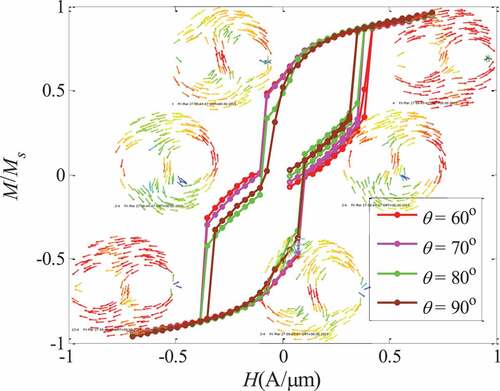
Figure 16. Hysteresis loop diagram of left vortex mechanism
Left vortex mechanism
The left vortex mechanism only appears when the aperture ratio and the angle
at which the magnetic field is applied. The hysteresis loop diagram of the left vortex mechanism is shown in (). When the applied forward magnetic field is large, the two-hole magnetic ring is saturated with positive magnetization, as the magnetic field decreases into the counterclockwise left vortex state, when the magnetic field decreases to zero and the reverse magnetic field is applied, the counterclockwise left vortex state does not flip to the counterclockwise right vortex state, but continues to increase with the reverse magnetic field into the reverse saturation state.
The magnetoelastic coupling has a significant effect on magnetization especially in multiferroic [Citation29,Citation30] and giant magnetostrictive materials [Citation31,Citation32]. Using the formula given by Zhang J X [Citation23] in 2005, with the magnetic elastic coupling energy items taken into consideration, the homogeneous strain can be roughly evaluated as:
where and
represent the volume average of
and
respectively. However, we consider it that in this paper the revolution of the magnetization is of key focus. The further effects of magnetoelastic coupling could be discussed in our future work.
The energy explanation of the evolutionary process of the magnetic domain
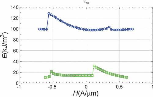
By extracting the energy density of various energies from the evolutionary process of the twin vortex mechanism, the left and right vortex mechanism and the ‘S’ mechanism, we analyze the demagation energy and exchange energy, investigate the change process of various energies in the evolutionary process, and explain the evolutionary process. We compare the twin-vortex reversal demagnetization energy with single hole ring (the magnetic field is gradually reduced from the forward maximum), as shown in (). Blue line is a two-hole ring twin-vortex flip and green is a single-hole ring flip. The single-hole ring and the double-hole ring form a closed vortex structure with a small magnetic field, which reduces the demagation energy, and the magnetic field of the twin-vortex has a wider range and is less affected by the external magnetic field, but a larger magnetic field needs to be applied when flipping. We compare twin-vortex flip exchange energy with single-hole ring, as shown in (). When the magnetic domain flips, the exchange energy will jump, indicating that the magnetic domain structure has changed.
Figure 17. Comparison of demagnetization energy of double-hole ring twin-vortex reversal mechanism and single-hole vortex reversal mechanism demagnetization energy (Blue line is double-hole ring and twin-vortex flip, green is single-hole ring vortex flip, the same below)
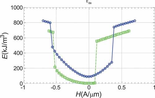
Figure 18. Comparison of the exchange energy of the double-hole ring twin-vortex flip mechanism and the exchange energy of the single-hole vortex flip mechanism
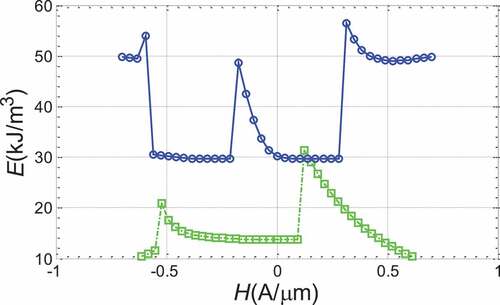
We also compare left and right vortex reversal demagnetization energy with single hole ring, shown in (). The energy of the left vortex and the right vortex of the double-hole magnetic ring is not much different, but adding holes makes the vortex state stay longer on the magnetic ring and the magnetic field range of the vortex state becomes larger. We compare exchange energy between left and right vortex flipping and single hole ring in (). The exchange energy of the double-hole magnetic ring undergoes three jumps during the unloading process of the magnetic field, and the magnetic domain structure undergoes three sudden changes, corresponding to the three jumps experienced by the four stable states of the hysteresis loop. Since the two 180° domain walls of the ‘S’ state rotate synchronously with the magnetic field loading on the edge of the ring, the magnetic domain area changes, so the magnetization of the ‘S’ evolution hysteresis loop changes with the magnetic field unloading. The magnetic field decreases, because the energy of the domain wall increases with the increase of the ring width. When rotating to a certain angle, the energy of the domain wall causes a sudden magnetization reversal, which turns from right to left to flow from left to right.
Figure 19. Comparison of the demagnetization energy of the double-hole ring left and right vortex reversal mechanism and the demagnetization energy of the single-hole vortex reversal mechanism (Blue is the double-hole ring with left and right vortex inversion, green is single-hole ring with vortex inversion, the same below)
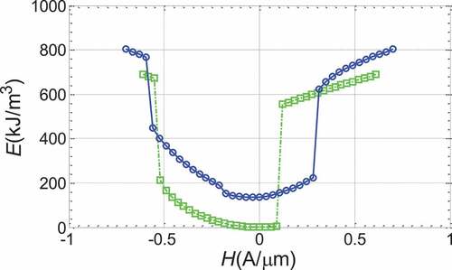
Figure 20. Comparison of the exchange energy between the left and right vortex flip mechanism of the double-hole ring and the exchange energy of the single-hole vortex flip mechanism
Application prospect of double-hole nanorings on random storage
Zhu J G [Citation33] in 2008 reviewed the different types of MRAM designs. Among them, there is a ring-based MRAM design, avoiding affection of geometric variation of the ends in actual fabrication on variation of the demagnetization field within the element. In the ring-based MRAM design, the magnetostatic flux forms a perfect closure, and the entire element has no demagnetizing field. In order to read the storage state, that is, the magnetization chirality in the storage layer, a bidirectional current pulse is injected into the ring element. The circular current field generated by the current will reverse the direction of the magnetization chirality in the integration according to the current layer. The magnetization chirality of the storage layer can then be determined by the corresponding magnetoresistance changes of the elements.
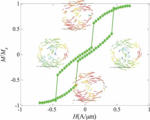
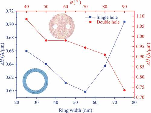
In this paper, we compare the magnetic field range of the double-hole ring twin-vortex state (TV) with the magnetic field range
of the single-hole ring vortex state (VT) with the same outer diameter and different ring widths, as shown in (), and find that the magnetic field range
of the double-hole ring twin-vortex state (TV) is greater than the magnetic field range
of the single-hole ring vortex state (VT), that is, the double-hole ring twin-vortex state (TV) is more stable than the single-hole ring vortex state (VT). The higher stability of the twin-vortex state (TV) of the double-hole ring makes the double-hole ring have greater advantages in high-density storage applications, such as: stored data is less likely to be lost and storage retention time is longer. Thus, twin-vortex evolution mechanism has the advantages of high stability and low demagnetization interference characteristics, and has good application prospects in magnetic random-access memory (MRAM).
Figure 21. Comparison of vortex stability of double-hole ring with twin-vortex and single-hole ring
Conclusion
In this paper, through the user subroutine element combining finite element and phase field, the magnetic domain evolution mechanism of the double-hole nanoring is studied, focusing on the mechanism of the magnetic domain affected by the geometric aperture and external magnetic field direction. Under different geometric apertures and external magnetic field direction parameters, we have found seven ways of magnetic domain evolution: twin-vortex mechanism, left and right vortex mechanism, ‘S’ evolution mechanism, ‘S’ + ‘C’ mechanism, ‘S’ + twin-vortex mechanism, ‘S’ + left vortex mechanism, left vortex mechanism. Due to the advantages of high stability and low demagnetization mutual interference, the twin-vortex mechanism has a good application prospect in random memory cells.
Acknowledgments
The authors acknowledge the support by the National Natural Science Foundation of China (Grant Nos. 12025201, 11521202, 11890681, 11522214). Calculations are supported by High-Performance Computing Platform of Peking University, China.
Disclosure statement
The authors declare that they have no conflict of interest.
Additional information
Funding
References
- Zhu JG, Zheng YF, Prinz GA. Ultrahigh density vertical magnetoresistive random access memory (invited). J Appl Phys. 2000;87(9):6668–6673.
- Schneider M, Hoffmann H, Zweck J. Magnetic switching of single vortex permalloy elements. Appl Phys Lett. 2001;79(19):3113–3115.
- Rothman J, Klaui M, Lopez-Diaz L, et al. Observation of a bi-domain state and nucleation free switching in mesoscopic ring magnets. Phys Rev Lett. 2001;86(6):1098–1101.
- Lai MF, Chang CR, Wu JC, et al. Magnetization reversal in nanostructured permalloy rings. IEEE Trans Magn. 2002;38(5):2550–2552.
- Moore TA, Hayward TJ, Tse DHY, et al. Magnetization reversal in individual micrometer-sized polycrystalline Permalloy rings. J Appl Phys. 2005;97(6):063910.
- Rahm M, Stahl J, Weiss D. Programmable logic elements based on ferromagnetic nanodisks containing two antidots. Appl Phys Lett. 2005;87(18):182107.
- Zhu FQ, Chern GW, Tchernyshyov O, et al. Magnetic bistability and controllable reversal of asymmetric ferromagnetic nanorings. Phys Rev Lett. 2006;96(2). DOI:10.1103/PhysRevLett.96.027205
- Mani AS, Geerpuram D, Baskaran VS, et al. Effect of controlled asymmetry on the switching characteristics of ring-based MRAM design. IEEE Trans Nanotechnol. 2006;5(3):249–254.
- Yang T, Hara M, Hirohata A, et al. Magnetic characterization and switching of Co nanorings in current-perpendicular-to-plane configuration. Appl Phys Lett. 2007;90:022504.
- Huang CH, Cheng NJ, Wu FS, et al. Study of vortex configuration and switching behavior in submicro-scaled asymmetric permalloy ring. IEEE Trans Magn. 2012;48(11):3648–3650.
- Hughes GF. Magnetization reversal in cobalt-phosphorus films. J Appl Phys. 1983;54(9):5306–5313.
- Fredkin DR, Koehler TR. Numerical micromagnetics by the finite-element method .2. J Appl Phys. 1988;63(8):3179–3181.
- Zhu JG, Bertram HN. Micromagnetic studies of thin metallic-films. J Appl Phys. 1988;63(8):3248–3253.
- Brunotte X, Meunier G, Imhoff JF. Finite-element modeling of unbounded problems using transformations - a rigorous, powerful and easy solution. IEEE Trans Magn. 1992;28(2):1663–1666.
- Miehe C, Ethiraj G. A geometrically consistent incremental variational formulation for phase field models in micromagnetics. Comput Methods Appl Mech Eng. 2012;245:331–347.
- Fredkin DR, Koehler TR. Hybrid method for computing demagnetizing fields. IEEE Trans Magn. 1990;26(2):415–417.
- Chen LQ. Phase-field models for microstructure evolution. Annu Rev Mater Res. 2002;32(1):113–140.
- Koyama T, Onodera H. Phase-field simulation of microstructure changes in Ni2MnGa ferromagnetic alloy under external stress and magnetic fields. Mater Trans. 2003;44(12):2503–2508.
- Wang J, Zhang J. A real-space phase field model for the domain evolution of ferromagnetic materials, International. J Solids Struct. 2013;50(22–23):3597–3609.
- Zhang H, Zhang X, Pei Y. A finite element based real-space phase field model for domain evolution of ferromagnetic materials. Comput Mater Sci. 2016;118:214–223.
- Muslov SA, Lotkov AI, Arutyunov SD. Extrema of elastic properties of cubic crystals. Russ Phys J. 2019;62(8):1417–1427.
- Dapino MJ. Magnetostrictive materials. In M. Schwartz: Encyclopedia of Smart Materials. New York, NY: John Wiley & Sons, Inc., 2002:600.
- Zhang JX, Chen LQ. Phase-field microelasticity theory and micromagnetic simulations of domain structures in giant magnetostrictive materials. Acta Materialia. 2005;53(9):2845–2855.
- Chung DH, Buessem WR. Elastic anisotropy of crystals. J Appl Phys. 1967;38(5):2010-&.
- Kube CM. Elastic anisotropy of crystals. AIP Adv. 2016;6(9):095209.
- Agarwal N. Characterization of lithographically patterned magnetic nanostructures. Arizona State University; 2007, 336E Orange St Tempe, AZ 85281.
- Rahm M, Stahl J, Wegscheider W, et al. Multistable switching due to magnetic vortices pinned at artificial pinning sites. Appl Phys Lett. 2004;85(9):1553–1555.
- Ha JK, Hertel R, Kirschner J. Micromagnetic study of magnetic configurations in submicron permalloy disks. Phys Rev B. 2003;67(22):224432.
- Chu Y-H, Martin LW, Holcomb MB, et al. Electric-field control of local ferromagnetism using a magnetoelectric multiferroic. Nat Mater. 2008;7(6):478–482.
- Bibes M, Barthelemy A. Multiferroics: towards a magnetoelectric memory. Nat Mater. 2008;7(6):425–426.
- Xu H, Pei Y, Fang D, et al. An energy-based dynamic loss hysteresis model for giant magnetostrictive materials, International. J Solids Struct. 2013;50(5):672–679.
- Xu H, Pei Y, Fang D, et al. Nonlinear harmonic distortion effect in magnetoelectric laminate composites. Appl Phys Lett. 2014;105:012904.
- Zhu J-G, Magnetoresistive random access memory: The path to competitiveness and scalability, Proceedings of the IEEE-Inst Electrical Electronics Engineers Inc, 96 (2008), pp. 1786–1798.