Optimal alignment for maximizing the uniaxial modulus of 2D anisotropic random nanofiber networks

ABSTRACT

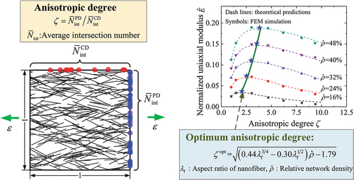
Nanofiber networks are effective structural forms to utilize the excellent nanoscale properties of nanofibers in macro scale. Properly tuning the anisotropic degree of fiber orientation distribution can maximize the macroscopic mechanical properties of random nanofiber networks in a specific direction. However, the reinforcing mechanism of the anisotropic orientation distribution to the elastic behavior has not been fully understood. In this paper, the effect of anisotropic orientation distribution of nanofibers on the elastic behavior of network is studied based on the modulus-density scaling relation and stiffness thresholds. The uniaxial modulus of network is determined by both the orientation angle of each fiber and interconnectivity of the random fiber network. With the increase of anisotropic degree, the contribution of fiber orientation angle to the network modulus of the preferential direction increases and gradually tends to a constant, while the interconnectivity of the networks decreases, which may reduce the loadability of network. Therefore, at a given network density, the uniaxial modulus along the preferential direction first increases to a maximum value and then decreases with the increase of the anisotropic degree. Furthermore, an expression to predict the optimal anisotropic degrees corresponding to the maximum uniaxial moduli at different network densities is established.

Graphical Abstract

KEYWORDS:

• Random nanofiber network
• nanofiber alignment
• uniaxial modulus
• stiffness threshold
• optimal design

1. Introduction

Networks assembled by randomly distributed nanofibers (such as carbon nanotubes) and their derived materials have a wide range of applications in many cutting-edge fields such as flexible electronics [1,2], strain sensors [3,4], artificial muscles [5,6], structural health monitors [7], and catalyst supports [8] due to their excellent chemical, electrical, mechanical, and optical properties, such as high specific stiffness and specific strength, high electrical/thermal conductivity, and transparence, which have attracted increasing attention in recent years.

As a kind of one-dimensional (1D) materials, the orientation distribution of nanofibers in networks significantly affects the macroscopic mechanical and electrical properties of networks [9–12]. Previous studies have shown that the slightly anisotropic nanofiber network could be easier to form connecting paths in networks to improve the mechanical [9,13–17] and electrical properties [13,14,17,18] in specific direction than isotropic network at the same density. For electrical conductivity of network at a certain density, it increases and then decreases with the increase of the degree of anisotropy [18–21]. As a result, there is an optimal anisotropic degree when the electrical conductivity along the preferential direction reaches its maximum [18]. Accordingly, it is reasonable to guess that the anisotropic nanofiber networks may have a similar optimal anisotropic degree at which the uniaxial modulus along the preferential direction reaches its maximum. Therefore, understanding the effect of nanofiber orientation distribution on the elastic behavior of network is of fundamental importance.

The elastic behaviors of isotropic nanofiber networks have been studied in the previous works [22–26]. It is found that the interconnectivity of randomly distributed short nanofibers plays an important role in the loadability of the network. With the increase of network density, the in-plane elastic behavior of nanofiber network presents three regimes that are linked by two critical network densities, i.e. the stiffness threshold and bending-stretching transitional threshold [25]. The former threshold is a criterion to judge whether the network can carry load, and the latter threshold is a criterion to measure whether most of the nanofibers can carry load efficiently by axial stretching/compression. Based on the two thresholds, the in-plane modulus can be concisely described by a three-regime piecewise formula. However, due to the limited efforts in theoretical and numerical investigations, there is still a lack of comprehensive understanding of the effect of nanofiber orientation distribution on the elastic behavior of networks. Furthermore, quantitative investigations of the optimal anisotropic degree still remain largely unexplored.

To this end, the effect of nanofiber orientation distribution on the elastic behavior of network is quantitatively studied. The investigation on the elastic behavior of anisotropic fiber networks is based on the modulus-density scaling relation with three key parameters. The anisotropic degree of fiber orientation distribution is evaluated with a simple single index that can be obtained by the geometric characteristics of the network, and named as anisotropic degree. Through systematically studying the effect of anisotropic degree on the three parameters of the modulus-density scaling relation, the uniaxial modulus of anisotropic network can be characterized analytically. Accordingly, the effect of anisotropic degree on the uniaxial modulus can be revealed, and an optimization on the anisotropic degree can be established.

2. Modeling and anisotropic degree of networks

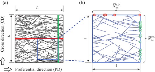
The elastic behavior such as the stiffness threshold and three-regime modulus-density scaling relation of 2-dimension (2D) and 3-dimension (3D) networks are similar [25], and the results of 2D networks can be calibrated to predict 3D networks [25,27]. Thus, a 2D mechanical model is firstly built to study the elastic behavior of nanofiber networks. The nanofibers are modeled as beams [28–31] and simplified as line segments with an identical length of l_f = 4 μm. The center point of each fiber is uniformly distributed in a squared representative area element (RAE) with a size of L = 20 μm, as shown in Figure 1a. The anisotropic degree can be controlled by the orientation angle of fibers θ. The fiber network is isotropic when orientation angle of fibers follows uniform distribution in the range of [-π/2, π/2). Here the periodic RAE is employed by periodicity processing [25].

Figure 1. Schematic diagrams of (a) the anisotropic nanofiber network and (b) the definition of fiber number densities on the cross-sections in the preferential direction and its cross direction.

Distinct from the macro scale counterparts, the interaction between nanofibers (e.g. carbon nanotubes) is an important factor affecting the elastic behavior of networks. Previous studies have shown that the non-bonded interactions of nanofibers, such as van der Waals interaction and physical entanglement, are too weak to transfer load efficiently [32]. To enhance the mechanical properties, stronger interactions such as nano-welding junctions [33–35] and chemical bonds [36] can be introduced. These connections can effectively restrain the relative sliding but can hardly provide a steady constraint to restrain the relative rotation between two nanofibers [25,37,38]. Thus, the interactions between nanofibers can be simplified as hinge connections [24,25]. Accordingly, the connection between two nanofibers is modeled as a hinge in this study.

The relative network density $\hat{\rho }$, defined as the projection area fraction of fibers in the RAE, is expressed as

(1) $\hat{\rho }=\frac{N_{\mathrm{f}}{l}_{\mathrm{f}}{d}_{\mathrm{f}}}{L^2}=\frac{n_{\mathrm{f}}{l}_{\mathrm{f}}^2}{{\lambda }_{\mathrm{f}}},$(1)

where N_f is the total number of fibers in the RAE, d_f = 0.01 μm is the diameter of the fiber, λ_f = l_f /d_f = 400 is the aspect ratio of fiber, and n_f = N_f/L² is the number density of fiber. The combined dimensionless parameter $n_{\mathrm{f}}{l}_{\mathrm{f}}^2$ can also be used to describe the network density, which is the average fiber number in the area of l_f×l_f.

To investigate the effect of nanofiber orientation distribution on the elastic behavior, the anisotropic networks are built. In experiments, the orientation distributions of nanofiber networks prepared by most preparation methods are similar to the Gaussian distribution (GD) [13,20,39,40], so that many studies use Gaussian distribution to describe the fiber orientation distribution [9,41]. Thus, the distribution law of the orientation angle of fiber θ is assumed to follow Gaussian distribution with a standard deviation σ_N around the preferential direction (PD). Here, the horizontal direction is taken as preferential direction for simplicity, as shown in Figure 1(a). The probability density function of the angle θ is expressed as

(2) $f\left(\theta \right)=\frac{1}{\sqrt{2\pi }{\sigma }_{\mathrm{N}}}exp\left(-\frac{{\theta }^2}{2{\sigma }_{\mathrm{N}}^2}\right),\theta \in \left[-\frac{\pi }{2},\frac{\pi }{2}\right]$(2)

The anisotropic degree increases with the decrease of the standard deviation σ_N.

To quantify the effect of anisotropic orientation distribution of the nanofibers, the anisotropic degree needs to be quantitatively characterized. Here the fiber number densities (i.e. fiber number per unit length/area) intersected by the cross-sections of the network are used. Considering the cross-sections that are perpendicular to the preferential direction and its cross direction (CD), the fiber number densities intersected by the two cross-sections can be denoted as ${\bar{N}}_{int}^{\mathrm{P}\mathrm{D}}$ and ${\bar{N}}_{int}^{\mathrm{C}\mathrm{D}}$, respectively, as shown in Figure 1b. The anisotropic degree of fiber networks can be defined as the ratio of ${\bar{N}}_{int}^{\mathrm{P}\mathrm{D}}$ to ${\bar{N}}_{int}^{\mathrm{C}\mathrm{D}}$, and expressed as

(3) $\zeta =\frac{{\bar{N}}_{\mathrm{i}\mathrm{n}\mathrm{t}}^{\mathrm{P}\mathrm{D}}}{{\bar{N}}_{\mathrm{i}\mathrm{n}\mathrm{t}}^{\mathrm{C}\mathrm{D}}}.$(3)

The anisotropic degree ζ is 1 when the material is isotropic, and it tends to positive infinity when the fibers are completely aligned. The fiber number densities for 2D networks can be obtained as

(4) ${\bar{N}}_{\mathrm{i}\mathrm{n}\mathrm{t}}=\frac{N_{\mathrm{i}\mathrm{n}\mathrm{t}}}{L},$(4)

where N_int is the number of fibers intersected by the cross sections of the RAE. Theoretically, the anisotropic degree can be derived as [25,42]

(5) $\zeta =\frac{{\int }_{-\frac{\pi }{2}}^{\frac{\pi }{2}}\left|cos\left(\theta \right)\right|f\left(\theta \right)\mathrm{d}\theta }{{\int }_{-\frac{\pi }{2}}^{\frac{\pi }{2}}\left|sin\left(\theta \right)\right|f\left(\theta \right)\mathrm{d}\theta }$(5)

In addition, for networks with straight fibers, the anisotropic degree ζ is equivalent to the ratio of the sum of fibers axes projections along the preferential direction to that along the cross direction [42].

3. Elastic behavior of anisotropic networks

For random nanofiber networks, the scaling relation between the uniaxial modulus and the relative network density can be expressed as [25]

(6) $\widehat{E}=0,0\widehat{\rho }\le {\widehat{\rho }}^{\text{S}1}\frac{k{\left(\widehat{\rho }-{\widehat{\rho }}^{\text{S}1}\right)}^2}{2\left({\widehat{\rho }}^{\text{S}2}-{\widehat{\rho }}^{\text{S}1}\right)},{\widehat{\rho }}^{\text{S}1}\widehat{\rho }{\widehat{\rho }}^{\text{S}2}k\left(\widehat{\rho }-\frac{{\widehat{\rho }}^{\text{S}1}+{\widehat{\rho }}^{\text{S}2}}{2}\right),\widehat{\rho }\ge {\widehat{\rho }}^{\text{S}2}$(6)

where $\hat{E}=\frac{E_{\mathrm{N}}}{E_{\mathrm{f}}}$ is the normalized uniaxial modulus, E_N is the effective modulus of network and E_f is the effective axial modulus of nanofiber, ${\hat{\rho }}^{\mathrm{S}1}$ and ${\hat{\rho }}^{\mathrm{S}2}$ are the stiffness threshold and bending-stretching transitional threshold of networks, respectively. Note that the effective axial modulus of nanofiber E_f shows obvious size dependence of the diameter in nanoscale [43–45], which is notwithstanding implicit in the normalization of $\hat{E}=\frac{E_{\mathrm{N}}}{E_{\mathrm{f}}}$, and should be paid attention when calculating the effective modulus of network E_N. The modulus of network can be divided into three regimes by the two thresholds: zero regime, bending dominated regime and stretching dominated regime. The modulus remains zero in the first regime, increases quadratically in the second regime, and then increases linearly with a slope k in the third regime [46]. This scaling relation is determined by the three parameters, i.e. ${\hat{\rho }}^{\mathrm{S}1}$, ${\hat{\rho }}^{\mathrm{S}2}$ and k. In the following, the effects of anisotropic degree on the three parameters are investigated, respectively. Besides, it should be noted that in this work we only focus on the linear elastic behavior of the networks under small deformation. When the deformation is large, the nanofibers are easy to buckle under axial compression, and thus the contribution of the buckled fibers to the macro loadability should be carefully reexamined [47].

3.1 Stiffness threshold of anisotropic networks

As another well-known threshold, the electrical percolation threshold has been intensively studied by both theoretical and experimental approaches [19,20,42,48–51]. Most researchers have reached a consensus that the electronics can be transferred if two nanofibers are contacted or connected by connections such as nano-welding junctions [33–35] or chemical bonds [36]. However, even if such a conductive path is formed, the constraint between two nanofibers is not sufficient for effective load-transfer [25,34]. Hence, the stiffness threshold that is higher than the electrical percolation threshold is required. In the previous studies, the stiffness threshold is defined as the critical network density at which almost all fibers in a network can carry load under an arbitrary loading [25]. However, this definition could not embody the effect of fiber orientation distribution and loading direction due to the relatively conservative estimation. For this reason, a new evaluation method based on load-carrying path is proposed through geometric probability analysis to predict the stiffness threshold for the anisotropic networks.

3.1.1 Load-carrying path

Forming connected and stable load-carrying paths (LCP) is a necessary and sufficient condition for the network to be loadable. To construct a load-carrying path, a mechanically stable configuration must be formed [52,53]. If three fibers intersect with each other and construct a triangle configuration with three connections, they are considered as stable fibers [54]. With the increase of fiber number, the initial stable triangle gradually grows to a stable cluster, and further constructs a connected load-carrying path spanning through the network.

Therefore, the load-carrying path should possess the following two features. (1) The fibers in the load-carrying path are stable, i.e. all fibers in the path can take part in carrying load. (2) The stable cluster in the load-carrying path rigidly connects two opposite edges of the network. In Figure 2, the stable and unstable fibers are demonstrated by solid and dashed line segments, respectively. The percolation process can be divided into three stages with the increase of network density, as shown in Figure 2a–c.

Figure 2. (a-c) The stiffness percolation process of 2D network with the increase of network density and (d) basic forms of small stable clusters (SSC), large stable clusters (LSC) and load-carrying paths (LCP).

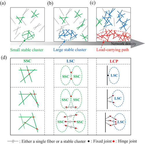
In the first stage, there are many small stable clusters (SSC) scattered in the network due to the low network density, as shown in Figure 2a. Then, with adding fibers into the network, the small stable clusters begin to coalesce into large stable clusters (LSC), as illustrated in Figure 2b. With the further increase of the network density, once a large stable cluster rigidly connects two opposite edges of network, this stable cluster is considered as a load-carrying path, and the network can carry load, as shown in Figure 2c. Note that the load-carrying path should link two opposite edges of the network, and thus it is directional.

Basic forms of SSC, LSC and LCP for 2D network are illustrated in Figure 2d. For the SSC, if (1) another fiber intersects with more than two fibers in the same stable triangle or stable cluster, or (2) two intersected fibers intersect with the same stable triangle or stable cluster, they are also stable and coalesce into the same stable cluster. For the LSC, if (1) more than two fibers in an SSC intersect with another SSC, or (2) a fiber in an SSC intersects with another SSC and a single fiber/stable cluster connects the two SSCs, or (3) more than three single fibers/stable clusters connect with the two SSCs, this two SSCs coalesce into an LSC. For the LCP, the stable cluster needs to be rigidly connected to the edges of the RAE. If (1) a fiber in LSC connects with the edge, or (2) more than two single fibers/stable clusters connect the LSC with the edge, or (3) more than three single fibers/stable clusters connect the LSC with the single fibers/stable clusters connected with the edge, the load on the edge can be transferred to stable cluster. If an LSC can rigidly connect to the two opposite edges of the RAE, the LSC is taken as an LCP.

3.1.2 Prediction of the stiffness threshold

Similar to the prediction of electrical percolation threshold [55,56], a process to determine the stiffness threshold is presented in this section. For a given network density, N_total samples of the RAE are generated randomly and then checked whether any load-carrying path is formed in the network. Denoting the number of networks with load-carrying path as N_L, the load-carrying probability P_L is defined as

(7) $P_{\mathrm{L}}=\frac{N_{\mathrm{L}}}{N_{\mathrm{t}\mathrm{o}\mathrm{t}\mathrm{a}\mathrm{l}}}.$(7)

Considering the calculation accuracy and efficiency, a converged relative size $\frac{L}{l_{\mathrm{f}}}=5$ is taken [25], and more than 250 network samples are simulated for each given network density. As shown in Figure 3a, the load-carrying probability P_L increases with the increase of network density, presenting an ‘S’ shape. This S-shaped curve can be described by Boltzmann function [25], and written as

Figure 3. (a) Relations between the load-carrying probability and the network density and (b) normalized stiffness thresholds of networks with different anisotropic degrees (λ_f = 400).

(8) $P_{\mathrm{L}}=P_{\mathrm{L}2}-\frac{P_{\mathrm{L}2}-P_{\mathrm{L}1}}{1+exp\left(\frac{\frac{\left(n_{\mathrm{f}}{l}_{\mathrm{f}}^2-C_0\right)}{dx}}{P_{\mathrm{L}2}-P_{\mathrm{L}1}}\right)}$(8)

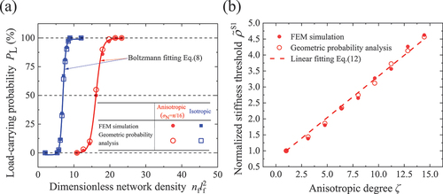
where P_L1 and P_L2 are the minimum and maximum values of P_L and should be set as 0% and 100%, respectively, C₀ is the horizontal coordinate of the center of the central symmetrical Boltzmann curve and satisfies the relation ${\left.P_L\right|}_{n_{\mathrm{f}}{l}_{\mathrm{f}}^2=C_0}=\frac{\left(P_{\mathrm{L}1}+P_{\mathrm{L}2}\right)}{2}$, and dx is the slope at the center point. The stiffness threshold is defined as the critical network density when the network is just able to carry load. Therefore, the network density at P_L = 50% is taken as the stiffness threshold.

For isotropic fiber network, the load-carrying probability P_L can be expressed as

(9) $P_{\mathrm{L}}=1-\frac{1}{1+exp\left(\frac{\left(n_{\mathrm{f}}{l}_{\mathrm{f}}^2-6.8\right)}{\mathrm{d}x}\right)}$(9)

The stiffness threshold of isotropic network can be obtained by Eq. (1)(1) $\hat{\rho }=\frac{N_{\mathrm{f}}{l}_{\mathrm{f}}{d}_{\mathrm{f}}}{L^2}=\frac{n_{\mathrm{f}}{l}_{\mathrm{f}}^2}{{\lambda }_{\mathrm{f}}},$(1) and Eq. (9(9) $P_{\mathrm{L}}=1-\frac{1}{1+exp\left(\frac{\left(n_{\mathrm{f}}{l}_{\mathrm{f}}^2-6.8\right)}{\mathrm{d}x}\right)}$(9) ), as

(10) ${\hat{\rho }}_{\mathrm{R}}^{\mathrm{S}1}=\frac{6.8}{{\lambda }_{\mathrm{f}}}$(10)

The electrical threshold of isotropic network can be obtained using the excluded volume method as ${\hat{\rho }}_{\mathrm{R}}^{\mathrm{E}}=\frac{5.8}{{\lambda }_{\mathrm{f}}}$ [48]. The stiffness threshold is about 1.17 times higher than the electrical percolation threshold, which is consistent with former studies [57]. This again indicates that more fibers are needed in the network to form the load-carrying path.

For simplicity, a normalized threshold ${\tilde{\rho }}^{\mathrm{S}1}$ is defined as the ratio of the stiffness threshold of anisotropic network ${\hat{\rho }}^{\mathrm{S}1}$ to that of isotropic network ${\hat{\rho }}_{\mathrm{R}}^{\mathrm{S}1}$, as

(11) ${\tilde{\rho }}^{\mathrm{S}1}=\frac{{\hat{\rho }}^{\mathrm{S}1}}{{\hat{\rho }}_{\mathrm{R}}^{\mathrm{S}1}}$(11)

The normalized stiffness threshold increases linearly with the increase of anisotropic degree, as shown in Figure 3b. The relation can be well fitted as

(12) ${\tilde{\rho }}^{\mathrm{S}1}=C_{\mathrm{S}1}\zeta +\left(1-C_{\mathrm{S}1}\right)$(12)

where C_S1 = 0.26 is obtained.

3.1.3 Numerical verification

To validate the prediction of stiffness threshold, finite element method (FEM) is employed here to calculate the uniaxial modulus of fiber networks using ABAQUS/Standard (2005) [24,25]. Here the geometric parameters of the FEM model are the same as those for the prediction by geometric probability analysis. In order to capture the essence of the nanofiber network structure and speed up the simulation, the mechanical behavior of the nanofibers can be simplified as elastic isotropic beams based on the continuum beam model [28,58,59]. The planar 3-node quadratic beam elements (B22 of Abaqus/Standard) are used in the simulation. The network modulus E_N can be obtained from the stress-strain relation of the network under the uniaxial tension. The network is stretched with given strain ε along the preferential direction, and the total reaction force along stretching direction F can be obtained. The network modulus E_N is then obtained as

(13) $E_{\mathrm{N}}=\frac{F}{\epsilon tL},$(13)

where the thickness of the network t is taken as t = d_f.

At a given network density around the stiffness threshold, the moduli calculated from FEM simulation can be divided into two groups according to their magnitudes. The moduli in one group are over 3 orders of magnitude larger than those in the other. The networks with higher moduli are considered to have load-carrying paths, while the others are considered to have no load-carrying path. Thus, the load-carrying probability P_L can also be taken as the ratio of the number of networks with higher moduli to the total number of network samples. As shown in Figure 3a, the load-carrying probabilities obtained by FEM simulation have good consistency with the results obtained by the geometric probability analysis for the isotropic and anisotropic networks. The stiffness thresholds of networks with different anisotropic degrees obtained by FEM simulation are shown in Figure 3b, and they all match well with the results obtained by the geometric probability analysis. Therefore, the prediction method of stiffness threshold based on load-carrying path is validated.

3.2 Bending-stretching transitional threshold

With the increase of network density after the stiffness threshold, the dominated deformation mode of fibers in networks changes from transverse bending to axial stretching, and the critical network density is defined as bending-stretching transitional threshold. The bending-stretching transitional threshold of isotropic fiber networks under uniaxial load has been investigated quantitatively in previous studies [25]. It is the network density when most of the deformation energy is induced by stretching/compression of the fibers, and can be obtained by fitting the modulus-density results of FEM simulation with Eq.(6)(6) $\widehat{E}=0,0\widehat{\rho }\le {\widehat{\rho }}^{\text{S}1}\frac{k{\left(\widehat{\rho }-{\widehat{\rho }}^{\text{S}1}\right)}^2}{2\left({\widehat{\rho }}^{\text{S}2}-{\widehat{\rho }}^{\text{S}1}\right)},{\widehat{\rho }}^{\text{S}1}\widehat{\rho }{\widehat{\rho }}^{\text{S}2}k\left(\widehat{\rho }-\frac{{\widehat{\rho }}^{\text{S}1}+{\widehat{\rho }}^{\text{S}2}}{2}\right),\widehat{\rho }\ge {\widehat{\rho }}^{\text{S}2}$(6) . For isotropic fiber network, the bending-stretching transitional threshold can be expressed as [25]

(14) ${\hat{\rho }}_{\mathrm{R}}^{\mathrm{S}2}=\frac{10.5}{{\lambda }_{\mathrm{f}}^{\frac{3}{4}}}.$(14)

Similarly, the normalized bending-stretching transitional threshold ${\tilde{\rho }}^{\mathrm{S}2}$ is used, and defined as

(15) ${\tilde{\rho }}^{\mathrm{S}2}=\frac{{\hat{\rho }}^{\mathrm{S}2}}{{\hat{\rho }}_{\mathrm{R}}^{\mathrm{S}2}},$(15)

where ${\hat{\rho }}^{\mathrm{S}2}$ is the bending-stretching transitional threshold of the anisotropic networks. As shown in Figure 4, the relation of the normalized bending-stretching transitional threshold and the anisotropic degree can also be well linearly fitted as

Figure 4. Normalized bending-stretching transitional threshold of networks with different anisotropic degrees (λ_f = 400).

(16) ${\tilde{\rho }}^{\mathrm{S}2}=C_{\mathrm{S}2}\zeta +\left(1-C_{\mathrm{S}2}\right).$(16)

Here C_S2 = 0.23 is obtained.

It can be found that both the stiffness threshold and bending-stretching transitional threshold increase with the increase of the anisotropic degree, which indicates that the interconnectivity of the network decreases, making it more difficult to form effective load-carrying paths.

3.3 Scaling relation of the whole range

The effect of nanofiber orientation distribution on the scaling relation between the normalized modulus and relative network density is shown in Figure 5a.

Figure 5. (a) The relations between the normalized uniaxial modulus and relative network density at different anisotropic degrees and (b) the slopes of the linear regime of $\hat{\rho }-\hat{E}$ curves for networks with different anisotropic degrees (λ_f = 400).

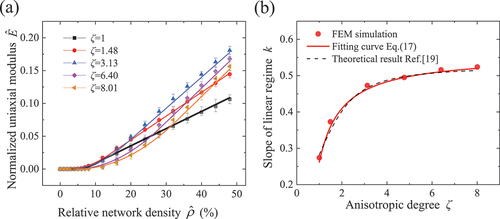
The normalized modulus of the anisotropic networks also presents three-regime form, i.e. zero regime, bending dominated regime, and stretching dominated regime. Accordingly, the normalized modulus of the anisotropic networks can also be expressed by the piecewise function of Eq.(6(6) $\widehat{E}=0,0\widehat{\rho }\le {\widehat{\rho }}^{\text{S}1}\frac{k{\left(\widehat{\rho }-{\widehat{\rho }}^{\text{S}1}\right)}^2}{2\left({\widehat{\rho }}^{\text{S}2}-{\widehat{\rho }}^{\text{S}1}\right)},{\widehat{\rho }}^{\text{S}1}\widehat{\rho }{\widehat{\rho }}^{\text{S}2}k\left(\widehat{\rho }-\frac{{\widehat{\rho }}^{\text{S}1}+{\widehat{\rho }}^{\text{S}2}}{2}\right),\widehat{\rho }\ge {\widehat{\rho }}^{\text{S}2}$(6) ), which only depends on the three parameters, the stiffness threshold ${\hat{\rho }}^{\mathrm{S}1}$, the bending-stretching transitional threshold ${\hat{\rho }}^{\mathrm{S}2}$ and the slope of linear regime of $\hat{\rho }-\hat{E}$ curve k. Subsections 3.1 and 3.2 have shown the effects of the fiber orientation distribution on the stiffness threshold and bending-stretching transitional threshold. The effect of the fiber orientation distribution on the slope of linear regime k is studied in the following part.

When the relative network density is higher than the bending-stretching transitional threshold, almost all fibers can carry load, and the dominated deformation mode of fiber is axial stretching/compression. As the further increase of the network density, and the modulus increases in a linear law [25]. The slope of the linear regime k can be obtained by fitting the $\hat{\rho }-\hat{E}$ curve from FEM simulations. With the increase of anisotropic degree, the slope first increases rapidly and then tends to a plateau, as shown in Figure 5b. It indicates that with the increase of anisotropic degree, the contribution of fiber orientation angle to the network modulus of the preferential direction first increases rapidly and gradually tends to a constant. The linear relation between the normalized modulus and relative density of the isotropic network is derived by Cox [46], and the slope of the linear regime k = π/12. Similarly, for anisotropic networks, theoretical results of k can also be derived for given orientation angle distributions [22], as shown in Figure 5b. By fitting the results, an approximate formulation of the slope of the linear regime of anisotropic networks can be well described as

(17) $k=\frac{\pi }{12}+C_{\mathrm{k}}\left(1-\frac{1}{\zeta }\right),$(17)

Here C_k = 0.30 is obtained.

Based on the above analysis, an expression to estimate the uniaxial modulus in preferential direction of the anisotropic networks can be established by substituting Eq.(12(12) ${\tilde{\rho }}^{\mathrm{S}1}=C_{\mathrm{S}1}\zeta +\left(1-C_{\mathrm{S}1}\right)$(12) ), Eq.(16)(16) ${\tilde{\rho }}^{\mathrm{S}2}=C_{\mathrm{S}2}\zeta +\left(1-C_{\mathrm{S}2}\right).$(16) , and Eq.(17)(17) $k=\frac{\pi }{12}+C_{\mathrm{k}}\left(1-\frac{1}{\zeta }\right),$(17) into Eq.(6(6) $\widehat{E}=0,0\widehat{\rho }\le {\widehat{\rho }}^{\text{S}1}\frac{k{\left(\widehat{\rho }-{\widehat{\rho }}^{\text{S}1}\right)}^2}{2\left({\widehat{\rho }}^{\text{S}2}-{\widehat{\rho }}^{\text{S}1}\right)},{\widehat{\rho }}^{\text{S}1}\widehat{\rho }{\widehat{\rho }}^{\text{S}2}k\left(\widehat{\rho }-\frac{{\widehat{\rho }}^{\text{S}1}+{\widehat{\rho }}^{\text{S}2}}{2}\right),\widehat{\rho }\ge {\widehat{\rho }}^{\text{S}2}$(6) ), as

(18) $\hat{E}=\left\{\begin{array}{cc}0,& 0<\hat{\rho }\le \left(C_{\mathrm{S}1}\zeta +\left(1-C_{\mathrm{S}1}\right)\right){\hat{\rho }}_{\mathrm{R}}^{\mathrm{S}1}\\ \frac{\left(\frac{\pi }{12}+\left(1-1/\zeta \right)C_k\right){\left(\hat{\rho }-\left(C_{\mathrm{S}1}\zeta +\left(1-C_{\mathrm{S}1}\right)\right){\hat{\rho }}_{\mathrm{R}}^{\mathrm{S}1}\right)}^2}{2\left(\left(C_{\mathrm{S}2}\zeta +\left(1-C_{\mathrm{S}2}\right)\right){\hat{\rho }}_{\mathrm{R}}^{\mathrm{S}2}-\left(C_{\mathrm{S}1}\zeta +\left(1-C_{\mathrm{S}1}\right)\right){\hat{\rho }}_{\mathrm{R}}^{\mathrm{S}1}\right)}& \left(C_{\mathrm{S}1}\zeta +\left(1-C_{\mathrm{S}1}\right)\right){\hat{\rho }}_{\mathrm{R}}^{\mathrm{S}1}<\hat{\rho }<\left(C_{\mathrm{S}2}\zeta +\left(1-C_{\mathrm{S}2}\right)\right){\hat{\rho }}_{\mathrm{R}}^{\mathrm{S}2}\\ \begin{array}{c}\left(\frac{\pi }{12}+\left(1-1/\zeta \right)C_k\right)\\ \times \left(\hat{\rho }-\frac{\left(C_{\mathrm{S}1}\zeta +\left(1-C_{\mathrm{S}1}\right)\right){\hat{\rho }}_{\mathrm{R}}^{\mathrm{S}1}+\left(C_{\mathrm{S}2}\zeta +\left(1-C_{\mathrm{S}2}\right)\right){\hat{\rho }}_{\mathrm{R}}^{\mathrm{S}2}}{2}\right)\end{array}& \hat{\rho }\ge \left(C_{\mathrm{S}2}\zeta +\left(1-C_{\mathrm{S}2}\right)\right){\hat{\rho }}_{\mathrm{R}}^{\mathrm{S}2}\end{array}\right.$(18)

Note that the influence of the aspect ratio of the fibers is implicit in the stiffness thresholds.

4. Optimal anisotropic degree at the maximum uniaxial modulus

For electrical conductivity of the anisotropic network at a certain network density, it increases to the maximum value and then decreases with the increase of anisotropic degree [18–21]. Similarly, this tendency also exists in the modulus, as shown in Figure 6. Therefore, the optimal anisotropic degree at the maximum modulus will be discussed.

Figure 6. Curves of normalized uniaxial modulus versus anisotropic degree at different network densities (λ_f = 400).

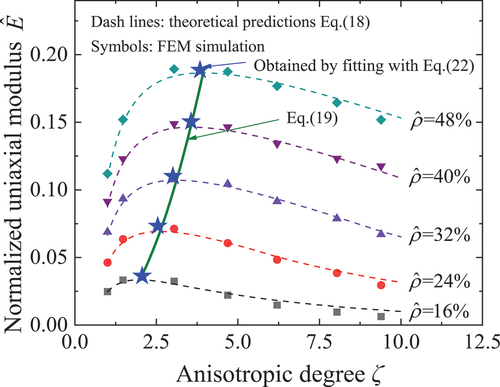
Previous studies have presented that the networks can carry load more efficiently when the dominated deformation mode of fibers is axial stretching/compression, i.e. when the network density is larger than the bending-stretching transitional threshold [25]. Therefore, we mainly focus on the optimal anisotropic degree in the stretching dominated regime. The optimal anisotropic degree can be obtained by the first derivative of Eq.(18(18) $\hat{E}=\left\{\begin{array}{cc}0,& 0<\hat{\rho }\le \left(C_{\mathrm{S}1}\zeta +\left(1-C_{\mathrm{S}1}\right)\right){\hat{\rho }}_{\mathrm{R}}^{\mathrm{S}1}\\ \frac{\left(\frac{\pi }{12}+\left(1-1/\zeta \right)C_k\right){\left(\hat{\rho }-\left(C_{\mathrm{S}1}\zeta +\left(1-C_{\mathrm{S}1}\right)\right){\hat{\rho }}_{\mathrm{R}}^{\mathrm{S}1}\right)}^2}{2\left(\left(C_{\mathrm{S}2}\zeta +\left(1-C_{\mathrm{S}2}\right)\right){\hat{\rho }}_{\mathrm{R}}^{\mathrm{S}2}-\left(C_{\mathrm{S}1}\zeta +\left(1-C_{\mathrm{S}1}\right)\right){\hat{\rho }}_{\mathrm{R}}^{\mathrm{S}1}\right)}& \left(C_{\mathrm{S}1}\zeta +\left(1-C_{\mathrm{S}1}\right)\right){\hat{\rho }}_{\mathrm{R}}^{\mathrm{S}1}<\hat{\rho }<\left(C_{\mathrm{S}2}\zeta +\left(1-C_{\mathrm{S}2}\right)\right){\hat{\rho }}_{\mathrm{R}}^{\mathrm{S}2}\\ \begin{array}{c}\left(\frac{\pi }{12}+\left(1-1/\zeta \right)C_k\right)\\ \times \left(\hat{\rho }-\frac{\left(C_{\mathrm{S}1}\zeta +\left(1-C_{\mathrm{S}1}\right)\right){\hat{\rho }}_{\mathrm{R}}^{\mathrm{S}1}+\left(C_{\mathrm{S}2}\zeta +\left(1-C_{\mathrm{S}2}\right)\right){\hat{\rho }}_{\mathrm{R}}^{\mathrm{S}2}}{2}\right)\end{array}& \hat{\rho }\ge \left(C_{\mathrm{S}2}\zeta +\left(1-C_{\mathrm{S}2}\right)\right){\hat{\rho }}_{\mathrm{R}}^{\mathrm{S}2}\end{array}\right.$(18) ), and expressed as

(19) ${\zeta }^{\mathrm{o}\mathrm{p}\mathrm{t}}=\sqrt{\frac{24C_{\mathrm{k}}\hat{\rho }+12C_{\mathrm{k}}\left(C_{\mathrm{S}1}{\hat{\rho }}_{\mathrm{R}}^{\mathrm{S}1}+C_{\mathrm{S}2}{\hat{\rho }}_{\mathrm{R}}^{\mathrm{S}2}-{\hat{\rho }}_{\mathrm{R}}^{\mathrm{S}1}-{\hat{\rho }}_{\mathrm{R}}^{\mathrm{S}2}\right)}{\left(\pi C_{\mathrm{S}1}+12C_{\mathrm{k}}{C}_{\mathrm{S}1}\right){\hat{\rho }}_{\mathrm{R}}^{\mathrm{S}1}+\left(\pi C_{\mathrm{S}2}+12C_{\mathrm{k}}{C}_{\mathrm{S}2}\right){\hat{\rho }}_{\mathrm{R}}^{\mathrm{S}2}}},\hat{\rho }\ge {\hat{\rho }}^{\mathrm{c}\mathrm{r}\mathrm{i}\mathrm{t}\mathrm{i}\mathrm{c}\mathrm{a}\mathrm{l}}$(19)

where ${\hat{\rho }}^{\mathrm{c}\mathrm{r}\mathrm{i}\mathrm{t}\mathrm{i}\mathrm{c}\mathrm{a}\mathrm{l}}$ is the critical relative network density, as detailed in Appendix A. Substituting the values of coefficients C_S1, C_S2 and C_k of the stiffness parameters in Eq.(19(19) ${\zeta }^{\mathrm{o}\mathrm{p}\mathrm{t}}=\sqrt{\frac{24C_{\mathrm{k}}\hat{\rho }+12C_{\mathrm{k}}\left(C_{\mathrm{S}1}{\hat{\rho }}_{\mathrm{R}}^{\mathrm{S}1}+C_{\mathrm{S}2}{\hat{\rho }}_{\mathrm{R}}^{\mathrm{S}2}-{\hat{\rho }}_{\mathrm{R}}^{\mathrm{S}1}-{\hat{\rho }}_{\mathrm{R}}^{\mathrm{S}2}\right)}{\left(\pi C_{\mathrm{S}1}+12C_{\mathrm{k}}{C}_{\mathrm{S}1}\right){\hat{\rho }}_{\mathrm{R}}^{\mathrm{S}1}+\left(\pi C_{\mathrm{S}2}+12C_{\mathrm{k}}{C}_{\mathrm{S}2}\right){\hat{\rho }}_{\mathrm{R}}^{\mathrm{S}2}}},\hat{\rho }\ge {\hat{\rho }}^{\mathrm{c}\mathrm{r}\mathrm{i}\mathrm{t}\mathrm{i}\mathrm{c}\mathrm{a}\mathrm{l}}$(19) ), the expression of optimal anisotropic degree can be expressed as

(20) ${\zeta }^{opt}=\sqrt{\frac{7.08{\lambda }_{\mathrm{f}}}{16.06{\lambda }_{\mathrm{f}}^{\frac{1}{4}}+11.86}\hat{\rho }-\frac{28.65{\lambda }_{\mathrm{f}}^{\frac{1}{4}}+17.79}{16.06{\lambda }_{\mathrm{f}}^{\frac{1}{4}}+11.86}},\hat{\rho }\ge \frac{209.62{\lambda }_{\mathrm{f}}^{\frac{1}{4}}+96.86}{16.21{\lambda }_{\mathrm{f}}+11.97{\lambda }_{\mathrm{f}}^{\frac{3}{4}}}$(20)

Generally, the aspect ratio of nanofiber ${\lambda }_{\mathrm{f}}$ is higher than 50, and the lower order terms of ${\lambda }_{\mathrm{f}}$ can be ignored. Therefore, the expression of optimal anisotropic degree can be rewritten as

(21) ${\zeta }^{opt}=\sqrt{\left(0.44{\lambda }_{\mathrm{f}}^{\frac{3}{4}}-0.30{\lambda }_{\mathrm{f}}^{\frac{1}{2}}\right)\hat{\rho }-1.79},\hat{\rho }\ge \frac{12.93}{{\lambda }_{\mathrm{f}}^{\frac{3}{4}}}$(21)

In addition, As shown in Figure 6, the normalized uniaxial modulus increases to the maximum value and then decreases gradually with the increase of the anisotropic degree. This trend could be also described by a lognormal function, as

(22) $\hat{E}={\hat{E}}^{\mathrm{o}\mathrm{p}\mathrm{t}}\cdot exp\left(-\frac{{\left(ln\left(\zeta \right)-{\mu }_{\mathrm{L}\mathrm{N}}\right)}^2}{2{\sigma }_{\mathrm{L}\mathrm{N}}^2}\right)$(22)

where ${\hat{E}}^{\mathrm{o}\mathrm{p}\mathrm{t}}$ is the maximum normalized uniaxial modulus of networks, and σ_LN and μ_LN are the standard deviation and mean of the lognormal function, respectively. The maximum modulus obtained by Eq.(22(22) $\hat{E}={\hat{E}}^{\mathrm{o}\mathrm{p}\mathrm{t}}\cdot exp\left(-\frac{{\left(ln\left(\zeta \right)-{\mu }_{\mathrm{L}\mathrm{N}}\right)}^2}{2{\sigma }_{\mathrm{L}\mathrm{N}}^2}\right)$(22) ) (blue pentagrams in Figure 6) are in good agreement with the theoretical results of Eq.(19)(19) ${\zeta }^{\mathrm{o}\mathrm{p}\mathrm{t}}=\sqrt{\frac{24C_{\mathrm{k}}\hat{\rho }+12C_{\mathrm{k}}\left(C_{\mathrm{S}1}{\hat{\rho }}_{\mathrm{R}}^{\mathrm{S}1}+C_{\mathrm{S}2}{\hat{\rho }}_{\mathrm{R}}^{\mathrm{S}2}-{\hat{\rho }}_{\mathrm{R}}^{\mathrm{S}1}-{\hat{\rho }}_{\mathrm{R}}^{\mathrm{S}2}\right)}{\left(\pi C_{\mathrm{S}1}+12C_{\mathrm{k}}{C}_{\mathrm{S}1}\right){\hat{\rho }}_{\mathrm{R}}^{\mathrm{S}1}+\left(\pi C_{\mathrm{S}2}+12C_{\mathrm{k}}{C}_{\mathrm{S}2}\right){\hat{\rho }}_{\mathrm{R}}^{\mathrm{S}2}}},\hat{\rho }\ge {\hat{\rho }}^{\mathrm{c}\mathrm{r}\mathrm{i}\mathrm{t}\mathrm{i}\mathrm{c}\mathrm{a}\mathrm{l}}$(19) .

5. Conclusions

In this work, the effect of fiber orientation distribution on the elastic behavior of random fiber network is quantitatively studied, and the optimal anisotropic degree at the maximum uniaxial modulus is quantified. The following conclusions can be drawn.

1) The criterion to judge whether the anisotropic network can carry load is reexamined. A new evaluation method based on load-carrying path is proposed to predict the stiffness threshold of anisotropic networks, which can embody the effect of fiber orientation distribution and loading direction, and is well validated by FEM simulation.

2) Similar to the isotropic counterpart, the three-regime elastic behavior with the increase of network density also exists in the anisotropic network, only with its three stiffness parameters affected. With the increase of anisotropic degree, the stiffness threshold and bending-stretching transitional threshold increase linearly, and the slope of the linear regime of modulus-density scaling relation increases and then converges to a constant. The relations between the anisotropic degree and the three stiffness parameters can be determined by three coefficients, respectively.

3) The uniaxial modulus of 2D anisotropic random nanofiber network does not monotonically increase with the increasing anisotropic degree (i.e. alignment degree) of nanofibers. At a given network density, the uniaxial modulus along the preferential direction increases to the maximum value and then decreases gradually with the increase of the anisotropic degree. Expression to predict the optimal anisotropic degree at the maximum uniaxial modulus is obtained theoretically and verified by FEM simulation.

Acknowledgments

Supports from the National Natural Science Foundation of China (Nos. 12002016, 12172026, and 12225201), the National Key Research and Development Program of China (No. 2020YFB1313003), the National Postdoctoral Program for Innovative Talents in China (No. BX20200032), the China Postdoctoral Science Foundation (No. 2020M680288), the Fundamental Research Funds for the Central Universities, and Beijing Advanced Discipline Center for Unmanned Aircraft System of China are gratefully acknowledged.

Disclosure statement

No potential conflict of interest was reported by the author(s).

Data Availability Statement

Data will be made available on request from the corresponding authors.

Additional information

Funding

This work was supported by the National Natural Science Foundation of China [12002016, 12172026, 2225201]; the National Key Research and Development Program of China [2020YFB1313003]; China Postdoctoral Science Foundation [2020M680288]; National Postdoctoral Program for Innovative Talents [BX20200032].

Appendix A.

Critical relative network density

The critical relative network density is

(A1) ${\hat{\rho }}^{\mathrm{c}\mathrm{r}\mathrm{i}\mathrm{t}\mathrm{i}\mathrm{c}\mathrm{a}\mathrm{l}}=\left[\frac{\left(-\pi C_{\mathrm{S}1}{C}_{\mathrm{S}2}{\hat{\rho }}_{\mathrm{R}}^{\mathrm{S}1}-\pi {\left(C_{\mathrm{S}2}\right)}^2{\hat{\rho }}_{\mathrm{R}}^{\mathrm{S}2}-12C_{\mathrm{k}}{C}_{\mathrm{S}1}{C}_{\mathrm{S}2}{\hat{\rho }}_{\mathrm{R}}^{\mathrm{S}1}+2\sqrt{\mathrm{A}}\right)}{\left(\pi C_{\mathrm{S}1}{\hat{\rho }}_{\mathrm{R}}^{\mathrm{S}1}+\pi C_{\mathrm{S}2}{\hat{\rho }}_{\mathrm{R}}^{\mathrm{S}2}+12C_{\mathrm{k}}{C}_{\mathrm{S}1}{\hat{\rho }}_{\mathrm{R}}^{\mathrm{S}1}+12C_{\mathrm{k}}{C}_{\mathrm{S}2}{\hat{\rho }}_{\mathrm{R}}^{\mathrm{S}2}\right)}+1\right]{\hat{\rho }}_{\mathrm{R}}^{\mathrm{S}2},$(A1)

where

(A2) $A=\sqrt{}3\pi C_{\text{k}}{\left(C_{\text{S1}}\right)}^2{\left(C_{\text{S2}}\right)}^2{\left({\widehat{\rho }}_{\text{R}}^{\text{S1}}\right)}^2-3\pi C_{\text{k}}{\left(C_{\text{S2}}\right)}^4{\left({\widehat{\rho }}_{\text{R}}^{\text{S2}}\right)}^2+36{\left(C_{\text{k}}\right)}^2{\left(C_{\text{S1}}\right)}^2{\left(C_{\text{S2}}\right)}^2{\left({\widehat{\rho }}_{\text{R}}^{\text{S1}}\right)}^2-3\pi C_{\text{k}}{C}_{\text{S1}}{\left(C_{\text{S2}}\right)}^2{\left({\widehat{\rho }}_{\text{R}}^{\text{S1}}\right)}^2+3\pi C_{\text{k}}{C}_{\text{S1}}{\left(C_{\text{S2}}\right)}^2{\widehat{\rho }}_{\text{R}}^{\text{S1}}{\widehat{\rho }}_{\text{R}}^{\text{S2}}-3\pi C_{\text{k}}{\left(C_{\text{S2}}\right)}^3{\widehat{\rho }}_{\text{R}}^{\text{S1}}{\widehat{\rho }}_{\text{R}}^{\text{S2}}+3\pi C_{\text{k}}{\left(C_{\text{S2}}\right)}^3{\left({\widehat{\rho }}_{\text{R}}^{\text{S2}}\right)}^2-36{\left(C_{\text{k}}\right)}^2{C}_{\text{S1}}{\left(C_{\text{S2}}\right)}^2{\left({\widehat{\rho }}_{\text{R}}^{\text{S1}}\right)}^2+36{\left(C_{\text{k}}\right)}^2{C}_{\text{S1}}{\left(C_{\text{S2}}\right)}^2{\widehat{\rho }}_{\text{R}}^{\text{S1}}{\widehat{\rho }}_{\text{R}}^{\text{S2}}-36{\left(C_{\text{k}}\right)}^2{\left(C_{\text{S2}}\right)}^3{\widehat{\rho }}_{\text{R}}^{\text{S1}}{\widehat{\rho }}_{\text{R}}^{\text{S2}}+36{\left(C_{\text{k}}\right)}^2{\left(C_{\text{S2}}\right)}^3{\left({\widehat{\rho }}_{\text{R}}^{\text{S2}}\right)}^2$(A2)

References

- Long G, Jin, WL, Xia, F, et al. Carbon nanotube-based flexible high-speed circuits with sub-nanosecond stage delays. Nat Commun. 2022;13(1):6734
- Jiang XW, Wang Z, Lu SW, et al. Vibration monitoring for composite structures using buckypaper sensors arrayed by flexible printed circuit. Int J Smart Nano Mater. 2021;12(2):198–217.
- Yan T, Wu Y, Tang J, et al. Flexible strain sensors fabricated using aligned carbon nanofiber membranes with cross-stacked structure for extensive applications. Int J Smart Nano Mater. 2022;13(3):432–446.
- Hu N, Masuda Z, Yan C, et al. The electrical properties of polymer nanocomposites with carbon nanotube fillers. Nanotechnology. 2008;19(21):215701.
- Foroughi J, Spinks GM, Wallace GG, et al. Torsional carbon nanotube artificial muscles. Science. 2011;334(6055):494–497.
- Liu X, Ji H, Liu B, et al. All-solid-state carbon-nanotube-fiber-based finger-muscle and robotic gripper. Int J Smart Nano Mater. 2022;13(1):64–78.
- Kang I, Schulz MJ, Kim JH, et al. A carbon nanotube strain sensor for structural health monitoring. Smart Mater Struct. 2006;15(3):737.
- Zhu W, Ku D, Zheng JP, et al. Buckypaper-based catalytic electrodes for improving platinum utilization and PEMFC’s performance. Electrochim Acta. 2010;55(7):2555–2560.
- Herasati S, Zhang L. A new method for characterizing and modeling the waviness and alignment of carbon nanotubes in composites. Compos Sci Technol. 2014;100(21):136–142.
- Stylianopoulos T, Bashur CA, Goldstein AS, et al. Computational predictions of the tensile properties of electrospun fibre meshes: effect of fibre diameter and fibre orientation. J Mech Behav Biomed Mater. 2008;1(4):326–335.
- Jiang X, Gong W, Qu S, et al. Understanding the influence of single-walled carbon nanotube dispersion states on the microstructure and mechanical properties of wet-spun fibers. Carbon. 2020;169:17–24.
- Firooz S, Steinmann P, Javili A. Homogenization of composites with extended general interfaces: comprehensive review and unified modeling. Appl Mech Rev. 2021;73(4). DOI: 10.1115/1.4050700
- Khan SU, Pothnis JR, Kim J-K. Effects of carbon nanotube alignment on electrical and mechanical properties of epoxy nanocomposites. Compos Part A Appl Sci Manuf. 2013;49:26–34.
- Wang Q, Dai J, Li W, et al. The effects of CNT alignment on electrical conductivity and mechanical properties of SWNT/epoxy nanocomposites. Compos Sci Technol. 2008;68(7–8):1644–1648.
- Ma D, Giglio M, Manes A. An investigation into mechanical properties of the nanocomposite with aligned CNT by means of electrical conductivity. Compos. Sci. Technol. 2020;188:107993.
- Moaseri E, Karimi M, Baniadam M, et al. Improvements in mechanical properties of multi-walled carbon nanotube-reinforced epoxy composites through novel magnetic-assisted method for alignment of carbon nanotubes. Compos Part A Appl Sci Manuf. 2014;64:228–233.
- Sun X, Chen T, Yang Z, et al. The Alignment of Carbon Nanotubes: an Effective Route To Extend Their Excellent Properties to Macroscopic Scale. Accounts Chem Res. 2013;46(2):539–549.
- Yook SH, Kim Y, Kim Y. Conductivity of stick percolation clusters with anisotropic alignments. J Korean Phys Soc. 2015;61(8):1257–1262.
- White SI, Didonna BA, Mu M, et al. Simulations and electrical conductivity of percolated networks of finite rods with various degrees of axial alignment. Phys Rev B. 2009;79(2):024301(1–6).
- Du F, Fischer JE, Winey KI. Effect of nanotube alignment on percolation conductivity in carbon nanotube/polymer composites. Phys Rev B. 2005;72(12):121404.
- Behnam A, Jing G, Ural A. Effects of nanotube alignment and measurement direction on percolation resistivity in single-walled carbon nanotube films. J Appl Phys. 2007;102(4):44313.
- Pan F, Zhang F, Chen Y, et al. In-plane and out-of-plane stiffness of 2D random fiber networks: Micromechanics and non-classical stiffness relation. Extreme Mech Lett. 2020;36:5.
- Pan F, Chen Y, Qin Q. Stiffness thresholds of buckypapers under arbitrary loads. Mech Mater. 2016;96:151–168.
- Pan F, Chen Y, Liu Y, et al. Out-of-plane bending of carbon nanotube films. Int J Solids Struct. 2017;106–107:183–199.
- Chen Y, Pan F, Guo Z, et al. Stiffness threshold of randomly distributed carbon nanotube networks. Journal of the Mechanics and Physics of Solids. 2015;84:395–423.
- Zhang M, Chen Y, Chiang FP, et al. Modeling the Large Deformation and Microstructure Evolution of Non-woven Polymer Fiber Networks. J Appl Mech Trans ASME. 2018;86:e45.
- Theodosiou TC, Saravanos DA. Numerical investigation of mechanisms affecting the piezoresistive properties of CNT-doped polymers using multi-scale models. Compos Sci Technol. 2010;70(9):1312–1320.
- Berhan L, Yi YB, Sastry AM, et al. Mechanical properties of nanotube sheets: alterations in joint morphology and achievable moduli in manufacturable materials. J Appl Phys. 2004;95(8):4335–4345.
- Lu P, Lee HP, Lu C, et al. Application of nonlocal beam models for carbon nanotubes. Int J Solids Struct. 2007;44(16):5289–5300.
- Wang X, Wang XY, Xiao J. A non-linear analysis of the bending modulus of carbon nanotubes with rippling deformations. Compos Struct. 2005;69(3):315–321.
- Ostanin I, Dumitrică T, Eibl S, et al. Size-Independent Mechanical Response of Ultrathin Carbon Nanotube Films in Mesoscopic Distinct Element Method Simulations. J Appl Mech Trans ASME. 2019;86(12). DOI: 10.1115/1.4044413
- Chen YL, Liu B, Hwang KC, et al. A theoretical evaluation of load transfer in multi-walled carbon nanotubes. Carbon. 2011;49(1):193–197.
- Piper NM, Fu Y, Tao J, et al. Vibration promotes heat welding of single-walled carbon nanotubes. Chem Phys Lett. 2011;502(4–6):231–234.
- Stormer BA, Piper NM, Yang XM, et al. Mechanical properties of SWNT X-Junctions through molecular dynamics simulation. Int J Smart Nano Mater. 2012;3(1):33–46.
- Kirca M, Yang X, To AC. Engineering, “A stochastic algorithm for modeling heat welded random carbon nanotube network. Comput Meth Appl Mech Engrg. 2013;259:1–9.
- Zhang J, Jiang D, Peng HX, et al. Enhanced mechanical and electrical properties of carbon nanotube buckypaper by in situ cross-linking. Carbon. 2013;63(63):125–132.
- Dai Z, Liu L, Qi X, et al. Three-dimensional Sponges with Super Mechanical Stability: harnessing True Elasticity of Individual Carbon Nanotubes in Macroscopic Architectures. Sci Rep. 2016;6(1):18930.
- Chen Y, Ma Y, Yin Q, et al. Advances in mechanics of hierarchical composite materials. Compos Sci Technol. 2021;214(1):108970.
- Fischer JE, Zhou W, Vavro J, et al. Magnetically aligned single wall carbon nanotube films: preferred orientation and anisotropic transport properties. J. Appl. Phys. 2003;93(4):2157–2163.
- Yang C, Li Q, Nie M, et al. Preferential alignment of two-dimensional montmorillonite in polyolefin elastomer tube via rotation extrusion featuring biaxial stress field. Compos Sci Technol. 2021;215:109034.
- Li Y, Stier B, Bednarcyk B, et al. The effect of fiber misalignment on the homogenized properties of unidirectional fiber reinforced composites. Mech Mater. 2016;92:261–274.
- Balberg I, Binenbaum N. Computer Study of the Percolation Thresold in a Two-Dimensional Anisotropic System of Conducting Sticks. Phys Rev B. 1983;28(7):3799–3812.
- Min KS, Sun IK, Kim SJ, et al. Size-dependent elastic modulus of single electroactive polymer nanofibers. Appl Phys Lett. 2006;89(23):231929–231929–3.
- McDowell MT, Leach AM, Gall K. On The Elastic Modulus of Metallic Nanowires. Nano Lett. 2008;8(11):3613–3618.
- Zhao J, Jiang JW, Wang L, et al. Coarse-grained potentials of single-walled carbon nanotubes. J Mech Phys Solids. 2014;71:197–218.
- Cox HL. The elasticity and strength of paper and other fibrous materials. British J of Applied Physics. 1951;3(3):72.
- Li C, Zhang Z, Zhan H, et al. Mechanical Properties of Single‐Layer Diamond Reinforced Poly (vinyl alcohol) Nanocomposites through Atomistic Simulation. Macromol Mater Eng. 2021;306(10):2100292.
- Balberg I, Anderson C, Alexander S, et al. Excluded volume and its relation to the onset of percolation. Phys Rev B. 1984;30(7):3933.
- Tarasevich YY, Eserkepov AV. Percolation of sticks: effect of stick alignment and length dispersity. Phys Rev E. 2018;98(6):062142.
- Mensah B, Kim HG, Lee J-H, et al. Carbon nanotube-reinforced elastomeric nanocomposites: a review. Int J Smart Nano Mater. 2015;6(4):211–238.
- Cui B, Pan F, Ding B, et al. Fiber Aggregation in Nanocomposites: aggregation Degree and Its Linear Relation with the Percolation Threshold. Materials. 2023;16(1):15.
- Ellenbroek WG, Mao X. Rigidity percolation on the square lattice. Europhys Lett. 2011;96(5):54002–54007.
- Jacobs DJ, Thorpe MF. Generic rigidity percolation in two dimensions. Phys Rev E. 1996;53(4):3682.
- Timoshenko SP, Young DH. Theory of structures. 2nd ed. New York: McGraw-Hill; 1965.
- Chang E. Percolation mechanism and effective conductivity of mechanically deformed 3-dimensional composite networks: computational modeling and experimental verification. Compos B Eng. 2021;207:108552.
- Chen Y, Wang S, Pan F, et al. A Numerical Study on Electrical Percolation of Polymer-Matrix Composites with Hybrid Fillers of Carbon Nanotubes and Carbon Black. J Nanomater. 2014;15:1–9.
- Latva-Kokko M, Timonen J. Rigidity of random networks of stiff fibers in the low-density limit. Phys Rev E. 2001;64:066117.
- Papanikos P, Nikolopoulos DD, Tserpes KI. Equivalent beams for carbon nanotubes. Comput Mater Sci. 2008;43(2):345–352.
- Wang XY, Wang X. Numerical simulation for bending modulus of carbon nanotubes and some explanations for experiment. Compos Part B Eng. 2004;35(2):79–86.