Nanoindentation in elastoplastic materials: insights from numerical simulations

Abstract

Finite element simulations of nanoindentation were performed on an elastoplastic material using Berkovich and conical indenters to investigate the effects of geometry on the load–displacement response of the material. The Berkovich indenter, widely used in nanoindentation experiments, is typically simplified to a theoretically equivalent 70.3° conical indenter for numerical simulations, which allows for a less computationally intensive two-dimensional (2D) axisymmetric analysis. Previous studies into the validity of this equivalence assumption for indentations in elastoplastic materials have varying conclusions. Using 2D and 3D finite element simulations, the present study investigates the response of elastoplastic materials, obeying a combined isotropic and kinematic hardening, to indentation with conical and Berkovich indenters. Simulations show that there is a clear difference in the load–displacement response of the selected material to the two indenters. The Berkovich geometry is found to produce a more localized pattern of contact stresses and plastic strains, leading to a smaller mobilized force for the same magnitude of displacement. To further validate the numerical simulations, experimental results of nanoindentation into an aluminium specimen were compared to elastoplastic finite element simulation results. Comparisons suggest that machining-induced residual stresses have likely affected the experimental results.

Keywords:

• nanoindentation
• finite element analysis
• elastoplasticity
• tip geometry

1. Introduction

Nanoindentation is an experimental method used to characterize materials at the nano and micro scale. During a nanoindentation test a diamond indenter tip is pressed into a material up to a specified force or depth and then withdrawn. As the test is performed, the indentation force and depth are recorded and results are normally presented in the form of a load–displacement curve. This load–displacement curve may be used to determine different material properties and characteristics [1,2]. An important factor in examining the results is the type of tip used in indentation. Berkovich indenters are one of the most common types of indenter tips used. A Berkovich tip is faceted in the form of a three-sided pyramid. Information relating to stress–strain behavior in an elastoplastic material during loading and unloading may be provided by finite element analysis. The commonly used Berkovich indenter with its three-sided pyramidal geometry must be modeled and analyzed as a three-dimensional (3D) contact problem in finite element simulations. However, the common approach in finite element simulation is to use a 2D axisymmetric indentation model, which uses a conical shaped indenter as an equivalent to a Berkovich indenter [3 –5]. The main reason for this approximation is that the 3D contact problem may require a large amount of computational resources and usually takes a long time to complete, especially when using a fine 3D mesh for accurate results. To overcome these challenges, a 70.3° half-angle conical indenter is often used as a substitute for modeling the Berkovich tip, on the basis that it provides the same indentation depth to projected area ratio of a Berkovich indenter. By using a conical indenter the finite element analysis can be simplified by using a 2D axisymmetric model, which allows for quicker simulations using fewer computer resources. Since this is a common approach for the finite element analysis of indentation problems, it is important to compare the finite element analysis results for both conical and Berkovich indentations to investigate any deviations in behavior between the two. Whereas there have been several recent studies comparing finite element simulations for the two indenters, the results presented by different investigators are not in full agreement.

One of the earliest studies that numerically compared different indenter tips was performed by Li et al. [6]. In their study, they compared several types of indenters, Berkovich, Vickers, and Knoop to several different conical indenters with half angles that were determined by different equivalency rules. The study provides simulations with indentation depth of approximately 1000nm in an elastoplastic material with isotropic hardening. The load–displacement curves obtained by Li et al. [6] show close agreement between the Berkovich result and the conical result with the Berkovich load being slightly higher in the mid range of indentation depth. The authors conclude that stress fields between Berkovich and conical indenters are different and if stress field is of interest, a 3D simulation is called for. However, if only load–displacement curve is needed then the Berkovich indenter can be sufficiently simulated by a conical indenter [6].

Swaddiwudhipong et al. [7] also attempted to address equivalency of Berkovich and conical indenters by performing 2D and 3D finite element analysis to simulate the load–displacement response in elastoplastic materials. Indentation simulations were performed for both conical and Berkovich indenters using different materials, including 6061 aluminum, that are set to obey power-law strain hardening. Indentations were simulated to a relatively deep 5 μm. A comparison is provided of load–displacement curves for conical and Berkovich indentations in 6061 aluminum. In this curve, the Berkovich indentation curve is noticeably lower than that of the conical indentation. The authors conclude that the equivalency between the two types of indenters in terms of the curvature of the load–displacement curve is not valid across the range of material properties considered [7].

Finite element simulations of nanoindentation in elastoplastic materials with no hardening were performed by Xu and Li [8] to study the effects of indenter geometry and mechanical properties of the indented material. The indenter geometries considered were conical and Berkovich. The study was specifically looking at correction factor but there are also plots that directly compare load–displacement behavior of both indenter types. In the provided plots, the Berkovich indentation curves are noticeably higher than those for the conical indenter across the range of material properties shown in the paper. The difference is explained as a geometry effect with the difference being more noticeable for harder materials [8].

Another investigation into the effect of indenter geometry on indentation test results was performed by Sakharova et al. [9]. Conical and Berkovich were among the indenter geometries examined. Elastoplastic indentations using Swift hardening law [10] were simulated using an in-house finite element code. The load–displacement plots obtained show that the responses from the different indenters were very similar. Small differences in the curves were observed when the ratio of the residual indentation depth after reloading and the indentation depth at maximum load (h _f/h _max) was below 0.65. In these cases, the Berkovich indenter curves were slightly higher [9].

Comparisons between the load–displacement responses of materials indented by conical and Berkovich indenters using finite element analysis have been presented in these earlier studies. However, the results do not seem to show a consistent trend, and therefore investigation into the equivalence between these two types of indenters is still incomplete.

The goal of this paper is to present a detailed finite element study of nanoindentation in order to gain additional insights into the effect of tip geometry on the force-displacement curves obtained in nanoindentation tests. The previous studies used different elastoplastic models including the use of different power-law hardening and the use of elastic-perfect plasticity. This study will investigate the behavior of conical and Berkovich indenters for materials obeying a combined isotropic and kinematic hardening.

2. Material modeling

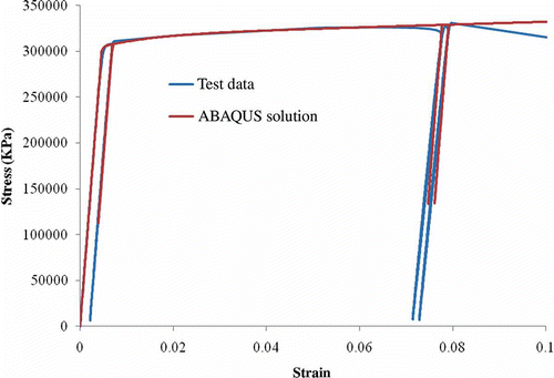
The experimental results and numerical simulations presented in this paper were performed on 6061 aluminum as a typical elastic–strain hardening plastic material. To evaluate the mechanical properties of this material, a macro scale uniaxial test was conducted and the observed stress–strain curve was used to calibrate the constitutive model used in the finite element analysis. All analyses were conducted using ABAQUS [11]. In ABAQUS, a metal plasticity constitutive model with combined isotropic/kinematic hardening was used to model the aluminum. Calibration of the combined isotropic/kinematic hardening model in ABAQUS requires half-cycle stress–strain test data. To acquire the required data, a uniaxial tension test was performed on a “dog bone” specimen of 6061 aluminum. During the test the sample was loaded in uniaxial tension, and once it reached initial yield stress the sample was unloaded and reloaded to yield again. The unloading and reloading process was repeated for two additional cycles. Stress and strain data were recorded throughout the test.

From the initial elastic loading data the Young's modulus (E) was calculated as approximately 65 GPa. A Poisson's ratio (ν) of 0.33 was assumed. Given the value of Young's modulus, the strain hardening data relating the yield stress to plastic strain were obtained from the test results. Table 1 shows the tabulated values of yield stress versus plastic strain. This data was used to calibrate the elastoplastic constitutive model. 

Table 1. Evolution of yield stress with plastic strain

Plastic strain	0.0	0.002	0.01605	0.04667	0.07511
Yield stress (kPa)	300,000	307,500	317,181	325,620	330,831

The calibration process was performed by conducting a plane stress simulation of a single finite element subjected to displacements that approximate those applied in the uniaxial tension test. After conducting a series of simulations and adjusting the number of back stresses to five for smoothing the elastoplastic transition, the finite element model provided a good simulation of the 6061 aluminum stress–strain behavior, as shown in Figure 1.

Figure 1. (Color online). Comparison of experimentally obtained stress–strain curves with the simulation of a combined isotropic/kinematic hardening plasticity model.

3. Finite element modeling

In this study, three different finite element nanoindentation models were investigated using the commercial finite element analysis program ABAQUS. The first model was a 2D axisymmetric model using a conical indenter. This type of model is commonly used in research and allows for relatively quick computation. The second model was a 3D finite element model with a conical indenter tip. This model, which is the full 3D equivalent to the 2D model, was used to confirm the suitability of the 3D finite element mesh. The third model was a 3D finite element mesh that included complete geometric representation of a Berkovich tip. This model allows for a thorough comparison of Berkovich tip to the assumed equivalent conic tip advocated in literature. Tip geometries for all the above models include a 200 nm tip radius to simulate a used indenter tip.

3.1. Verification of the 2D finite element model

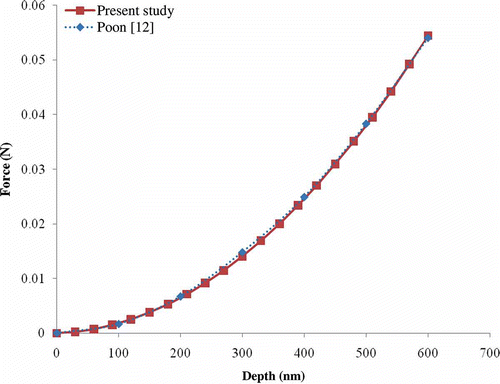
The first step was to create and verify a 2D axisymmetric nanoindentation model in ABAQUS. The performance of the developed model was verified against the available results in literature. As part of his doctorate thesis, Poon [12] performed a series of finite element simulations of elastic indentations while adjusting the radius and height of the specimen. These simulations suggest the proper specimen size to approximate a body of semi-infinite extent for a given indentation depth. Reproducing the key results of Poon's simulation helped verify the quality of the finite element mesh and the sizing of the material dimensions used in the present study.

Poon [12] initially provided a simulation for an axisymmetric indentation onto the top surface of a cylindrical specimen with a radius, r _s, of 18 μm and a height, h _s, of 30 μm. The specimen was modeled as an elastic isotropic deformable solid with E = 70 GPa and ν = 0.3. The 70.3° half-angle “Berkovich equivalent” conical indenter was modeled as an analytical rigid surface with a tip radius of ρ = 200 nm. The maximum indentation depth was h _max = 600 nm. The finite element mesh was described as using 5006 three-node linear axisymmetric triangular elements (CAX3) with a higher mesh density at the indentation site. For later simulations the number of nodes was scaled depending on the specimen dimensions. Contact between the indenter and specimen was modeled as frictionless.

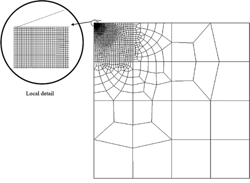
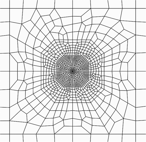
A 2D axisymmetric model was created for the present study using the same parameters detailed in [12]. While CAX3 element type was used, a different finite element mesh was constructed to see the potential effects of mesh configuration. The specimen was modeled with editable dimension constraints for the radius and height. The face of the specimen was then partitioned into quarters. In order to easily provide a higher density mesh at the indentation site, the quadrant containing the indentation site (upper left) was quartered. This last step was repeated until the face in the corner of the indentation site was sufficiently small. The resulting face partition of the specimen is shown in Figure 2. Edges were then seeded to provide a high mesh density at the indentation site and less density further away, as shown in Figure 3.

Figure 2. Face partitioning of 2D axisymmetric specimen.

Figure 3. 2D axisymmetric finite element mesh of the specimen.

A linear elastic analysis was performed using the same material size and specifications used in the initial Poon's simulation. Figure 4 shows the load–displacement result obtained from this simulation and compares it to the simulation result presented in [12]. The curves were in good agreement with only slight differences which may be caused by errors in reading the values from the curves in [12].

Figure 4. (Color online). Load–displacement comparison for elastic indentation simulation into a specimen with r _s = 18 μm and h _s = 30 μm.

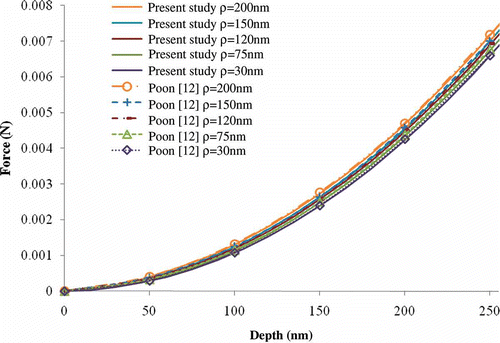
The results presented by Poon [12] are shown for the range of indentation of approximately 260 nm, though the actual indentation depth is not given. To reproduce the results for this study, an indentation depth of 300 nm was used on a material with r _s = 30 μm and h _s = 30 μm. Load–displacement results are shown in Figure 5. The results show good agreement in values and trends when compared with those obtained by Poon [12].

Figure 5. (Color online). Load–displacement comparison for elastic indentation simulation into a specimen with varying indenter tip radii, ρ (30, 705, 120, 150 and 200 nm).

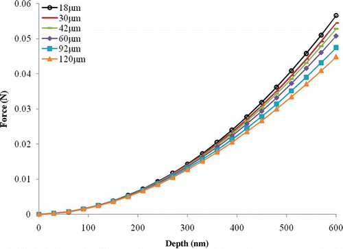
Simulations were also performed keeping the same specimen radius of r _s = 18 μm, while varying the specimen height, h _s, through the values 18, 30, 40, 60, 92 and 120 μm. The load–displacement results for the simulations are shown in Figure 6. The results exhibit the expected trend where load increases with decreased specimen height.

Figure 6. (Color online). Load–displacement curves for elastic indentation simulation into a specimen with r _s = 18 μm and varying h _s (18, 30, 42, 60, 92 and 120 μm).

For further simulations in the study, the material dimensions are chosen to be r _s = 60 μm and h _s = 60 μm to accommodate indentations of up to 600 nm according to the convergence relations provided.

3.2. 2D and 3D elastoplastic simulations

The 2D axisymmetric finite element mesh was verified for elastic indentation. To perform elastoplastic indentations the calibrated elastoplastic constitutive model was used. The material specimen was sized to accommodate indentations up to a 600 nm. The element type in the mesh was changed to a four-node bilinear axisymmetric quadrilateral element (CAX4R), which for linear elastic analysis would produce the same results as those obtained by the CAX3 element used in verification studies discussed earlier.

Initial elastoplastic simulations resulted in load–displacement curves that exhibited a slight oscillation or “stepping type” behavior in the load–displacement curve. This behavior was corrected by providing a more uniform grid for the fine mesh around the indentation site. The mesh was verified through a convergence study of the 2D elastoplastic indentation, as shown in Figure 7.

Figure 7. (Color online). Comparison of the simulations using different 2D axisymmetric finite element meshes in elastoplastic indentation.

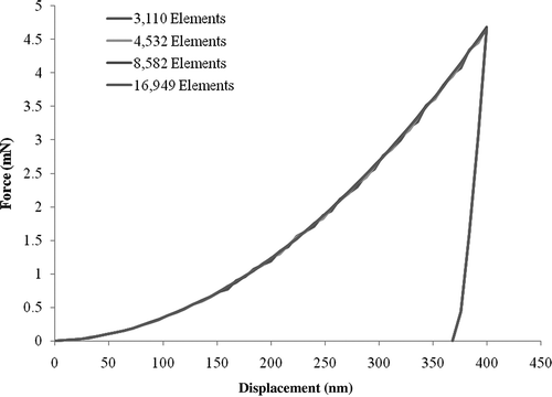
The final mesh chosen included 8582 elements. The 2D analysis results were later used as a baseline for comparison against the 3D indentation models. Figure 3 shows the 2D axisymmetric mesh with a detail of the local mesh near the indenter tip.

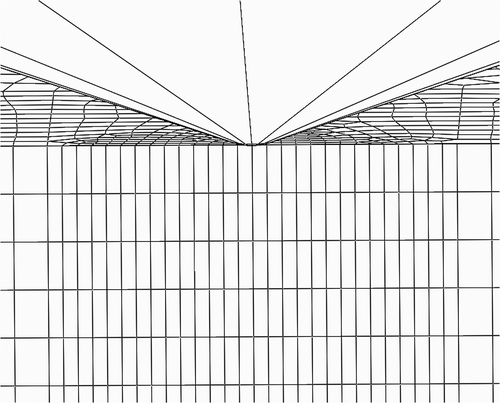
To provide confirmation of the suitability of 3D meshes and for direct comparison to the 2D model, a 3D conical tip nanoindentation model was first created. Similar to the 2D model, the 3D indentation model was created using a 70.3° half-angle Berkovich equivalent cone. The conical indenter was created as a revolved shell analytical rigid surface. The specimen was created in a cylindrical shape with the same depth and radius as the 2D axisymmetric model and elastoplastic material parameters were also identical to those used in the 2D axisymmetric model. The finite element mesh of the specimen was created so that it is fine on the surface around the site of indentation as well as the initial depth of the cylinder. The mesh was then increasingly coarsened in the areas that were further away from the indentation site. Each quadrant of the specimen's top surface was meshed by using a method similar to that used in the 2D axisymmetric model, i.e. creating increasingly smaller square partitions and then seeding the edges for desired mesh density. The element type was chosen to be an eight-node linear brick using reduced integration and hourglass control (C3D8R). Figure 8 shows the 3D finite element mesh and a local mesh detail near the tip is shown in Figure 9.

Figure 8. 3D finite element mesh of the specimen.

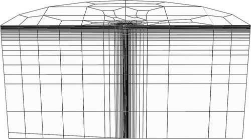
Figure 9. Local details of 3D finite element mesh near the indenter.

A 3D Berkovich tip nanoindentation model was the third and final finite element mesh created for analysis and comparison. The material model and the finite element mesh of the specimen were carried over from the conical simulation. The main difference between the two 3D models was the tip geometry. The Berkovich tip was modeled as a three sided pyramid with a semi-angle between vertical and each face of 65.27°. An area of difficulty in modeling the Berkovich tip was in the process of rounding the tip. A pyramidal shape cannot be tangentially rounded by a sphere along all sides and edges. Instead the tip was rounded using the intersection between a sharp Berkovich geometry and a conical geometry with a 200 nm tip radius and a half angle of 70.3°, which is equivalent to the semi-angle to the sharp edges of a Berkovich pyramid. Due to the complexity in the Berkovich tip geometry it cannot be treated as an analytical rigid surface, instead it was modeled as a discrete rigid surface.

After some preliminary simulations, slight adjustments were made to the specimen mesh for the Berkovich indentation to accommodate interaction with the more complicated Berkovich tip geometry. Distortions in the mesh would arise depending on the orientation of elements that were contacted by the pyramid edge. The mesh was modified in the region of tip contact to align element edges with the pyramid edges. This correction reduced mesh distortion and provided an improvement in the load–displacement response. A local detail of the improved mesh configuration is shown in Figure 10.

Figure 10. Local top surface details of the modified 3D finite element mesh configured to improve interaction with Berkovich indenter.

All three finite element models shared several common characteristics. The elastoplastic material properties used were those obtained from the uniaxial tension test of 6061 aluminum. Contact was modeled as frictionless between the indenter and material. Displacement of the indenter was applied through a displacement boundary condition applied to a reference node of the rigid indenter surface. Indentation force was obtained by requesting output of the reaction force at the reference node during the analysis.

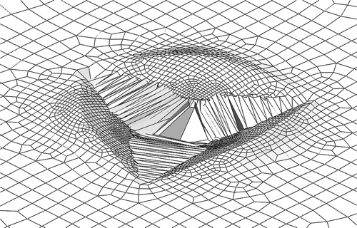
Results in the study were all obtained from ABAQUS implicit analysis. However, explicit analysis was also considered. Simulation results revealed that explicit analysis would work well for analysis of a 3D cone since it provided a response very similar to that of the implicit analysis. However, the explicit analysis provided poor results for the Berkovich indentation. The poor performance was attributed to large elemental distortion of the material in regions of the mesh that had contact interaction with the edges of the Berkovich pyramid. This led to a decrease in simulation accuracy with increased mesh refinement due to larger relative distortions for the finer elements. These large distortions not only led to inaccuracy but the unexpected behavior where the material would pull back on the indenter resulting in a negative reaction force during unloading. Figure 11 shows an example of the mesh distortion experienced in an explicit analysis. Implicit analysis was confirmed to be the preferable method for nanoindentation simulation.

Figure 11. Mesh distortion observed in explicit simulation of Berkovich indentation.

Using these three finite element models, a comparison of how geometry affects the indentation results can be made. The main point of interest was how similar the load–displacement behavior was between a Berkovich indenter and the equivalent conical indenter.

4. Results and discussion

4.1. Finite element simulations of nanoindentation

The results were first examined by considering the load–displacement curves of the elastoplastic indentation process. The load–displacement curve represents the overall material reaction to the nanoindentation process and it also represents what would be recorded during a nanoindentation experiment. An indentation depth of 400 nm was chosen in this comparison study.

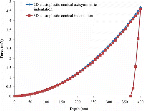
Figure 12 compares the load–displacement results obtained from a 2D axisymmetric conical indentation simulation and a 3D conical indentation simulation. It would be expected that both simulations would provide the same curve. In line with expectations, the two curves are in good agreement with each other. At maximum indentation depth the difference between the two curves is less than 2%. The differences may be attributed to the fact that the mesh of the 2D axisymmetric model is much finer than the 3D conical model in the area around the tip. Increasing the mesh refinement in the 3D model would lead to significant increases in simulation time while producing little improvement in the simulation results. Hence, the 3D finite element mesh was considered to be sufficiently refined.

Figure 12. (Color online). Comparison of load–displacement curves for 2D and 3D conical indentations.

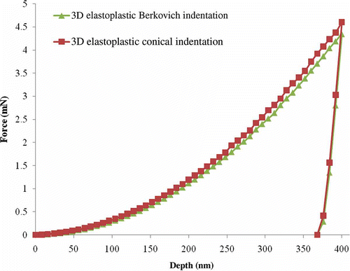
Figure 13 shows a comparison of the load–displacement curves for the Berkovich and conical indenters. It can be seen that there is a difference between the results. The Berkovich indentation curve is noticeably lower than that of the conical indenter.

Figure 13. (Color online). Comparison of load–displacement curves for conical and Berkovich indentations.

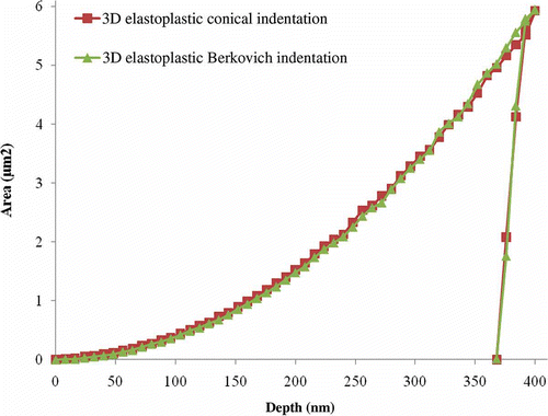
According to common practice the curves should match if the projected area to indentation depth is equal. The contact area during indentation was then checked for both indenter geometries to determine if there are differences in contact area that are leading to load differences. Figure 14 shows the contact area for both Berkovich and conical indenters as it relates to indentation depth in the simulations. The contact area curves for the two indenters have slight differences but in general they are very similar to each other.

Figure 14. (Color online). Comparison of contact areas computed in conical and Berkovich indentations.

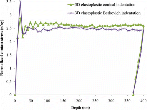
The contact areas for Berkovich and conical indenters are essentially the same but their load–displacement curves have noticeable differences; this provides good motivation to examine the normalized contact stresses for the two indenters. The normalized contact stresses during indentation for the two indenters is shown in Figure 15. Both curves share the same initial elastic loading during contact initiation; however, after the transition into the plastic regime the curve for the normalized stress for the Berkovich indenter is consistently lower than the curve for the conical indenter. There seems to be a geometry effect that is resulting in different indentation responses for the two indenters.

Figure 15. (Color online). Comparison of normalized contact stresses computed for conical and Berkovich indentations.

To further examine the potential effect of geometry during the elastoplastic indentation, finite element visualizations were utilized to examine the material behavior around the indentation site. Figure 16a shows the Mises stress field for the 70.3° conical indenter at maximum indentation depth. The axisymmetric geometry of the conical indenter provides an axisymmetric stress field. Figure 16b shows the Mises stress field for the Berkovich indenter with a view cut in the plane perpendicular to a sharp edge of the pyramid which provides an angle similar to that of the equivalent cone. On this cross-section, the stress fields between the two indenters are quite similar.

Figure 16. (Color online). Mises stress for (a) 70.3° conical indenter, (b) Berkovich indenter, viewed in plane perpendicular to indenter edge, and (c) Berkovich indenter, viewed in plane of indenter edge. (Figure continued).

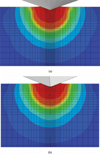
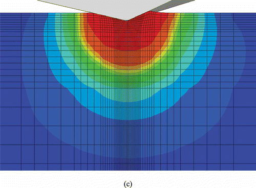
Figure 16c shows the Mises stress field for the Berkovich indenter with a view cut made in the plane of a sharp edge of the pyramid which provides the cross-section with the most dissimilar angle. On this cross-section the stress field extends noticeably further laterally on the side of the flat edge of the pyramid and does not extend as far near the sharper edge.

The distribution of equivalent plastic strain which depends on the material model was also examined. Figure 17a shows the equivalent plastic strain distribution on the material surface after conical indentation. The maximum equivalent plastic strain for the conical indentation was 170%. The distribution of equivalent plastic strain for the Berkovich indentation is shown in Figure 17b. For the Berkovich indentation the maximum equivalent plastic strain was 204% for the same indentation depth as that in conical indentation.

Figure 17. (Color online). Contours of equivalent plastic strain for (a) 70.3° conical indenter and (b) Berkovich indenter.

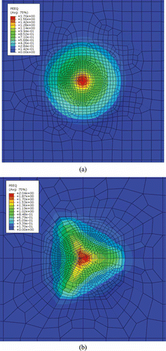
It can be seen from the strain distribution that the edges of the pyramid contribute to creating higher equivalent plastic strains in the Berkovich indenter than those experienced by the conical indenter.

Despite the contact area being the same throughout the indentation process for both indenters, the material is responding differently due to geometry effects. The edges of the Berkovich's pyramidal geometry induce higher plastic strains. This means that for the Berkovich indenter there is more localized yielding in the material. With more localized yielding the material is less resistant to penetration which results in lower required indentation loads for the Berkovich indenter compared to the 70.3° conical indenter.

4.2. Comparison of simulations with nanoindentation experiments

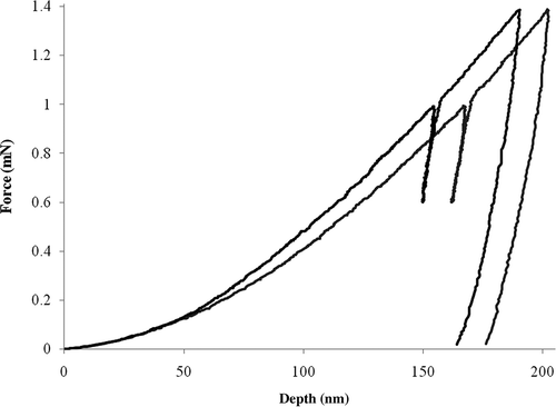
To assess the validity of numerical simulations, it is always desirable to compare them with the observed responses of the material in nanoindentation experiments. This will also provide additional confidence regarding the ability of the finite element analysis to accurately predict a real nanoindentation test result. Hence, a cylindrical specimen was prepared for the nanoindentation test using the same type of aluminum used in calibration of the finite element model. A series of nanoindentation tests were performed using an Asylum Research MFP-3D™ stand-alone atomic force microscope (AFM) fitted with a nanoindenter module (Asylum Research, Santa Barbara, CA). A series of 64 indentations were performed in a grid pattern on the material surface and a sampling of curves showing the variation in load–displacement response among the indentations is shown in Figure 18. The indentations were performed using force control to a maximum indentation force of 1.4 mN. The variation in indentation depth is thought to be from variations in the material properties due to the effects of machining the sample.

Figure 18. Upper and lower bounds of experimental load–displacement curves.

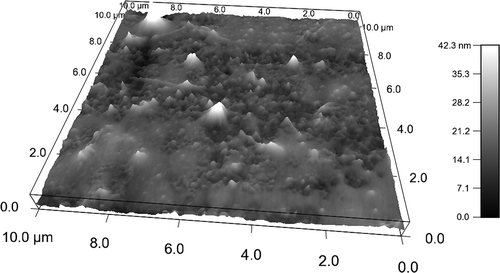
An AFM-produced contour plot of the material surface is shown in Figure 19. The surface roughness for this 100 μm² plot was given as approximately 3.5 nm.

Figure 19. AFM-produced contour plot of specimen surface.

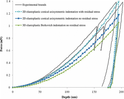
Performing finite element simulations to a maximum depth similar to experimental values for both the conical and Berkovich indenters resulted in load–displacement curves with significantly lower loads compared to experimental values. Warren and Guo [13] discuss that machining-induced residual stress can significantly affect load–displacement curves. The residual stresses may be estimated through finite element simulation. In their sample of 52100 steel, residual stresses were estimated to be 18% of yield stress in the horizontal direction and 12% of yield stress in the vertical direction. These values were used as a starting point in estimating the residual stresses in the aluminum specimen in the present study.

Using the 2D axisymmetric finite element model (due to its less computational effort) a series of simulations were performed while adjusting residual stress parameters. The residual stresses were estimated to be approximately 8% of yield stress in the horizontal direction and 5% of yield in the vertical direction. Incorporating these residual stresses as the initial stresses was shown to bring up the computed load–displacement curves well within the experimental bounds. Figure 20 compares the conical and Berkovich indentations without residual stresses, the conical indentation with residual stresses, and the experimental bounds.

Figure 20. (Color online). Comparison of numerically obtained force–displacement curves with experimental bounds.

5. Conclusions

Finite element simulations of elastoplastic nanoindentations were performed for conical (70.3°) and Berkovich indenters to study the effect of indenter geometry on the response of an elastoplastic material. It is shown that there are clear differences in the load–displacement responses between the two indenters. Loads in the Berkovich indentation are noticeably lower. It is confirmed that contact areas during indentation are very similar, resulting in lower normalized contact stress for the Berkovich indenter. Examination of stress fields near the indenter tip shows that the symmetrical cross-sections of the Berkovich indenter are similar to the axisymmetric stress field of the conical indenter and differences arise when compared to asymmetric cross-sections of the Berkovich indenter. Maximum equivalent plastic strain induced by indenter is demonstrated to be 20% higher for the Berkovich indenter. It is concluded that higher localized plastic strains would result in less resistance to indentation by the material and explain the load–displacement behavior. The results reveal that the use of a 70.3° conical indenter to approximate the response from a Berkovich indenter is not valid for all materials.

The ability of finite element analysis to predict experimental nanoindentation results was also examined. Comparisons with experimental results suggest that machining-induced residual stresses have likely affected the experimental results. It is also demonstrated that these residual stresses may be estimated by matching simulated load–displacement curves within the range of experimental curves.

Acknowledgment

This work was supported in part by the Air Force Office of Scientific Research under Award No. FA9550-09-0268. This support is greatly appreciated.

References

- Oliver , W.C. and Pharr , G.M. 2004 . Measurements of hardness and elastic modulus by instrumented indentation: Advances in understanding and refinements to methodology . J. Mater. Res. , 19 : 3 – 20 .
- Mencik , J. 2007 . Determination of mechanical properties by instrumented indentation . Meccanica , 42 : 19 – 29 .
- Knapp , J.A. , Follstaedt , D.M. , Myers , S.M. , Barbour , J.C. and Friedmann , T.A. 1999 . Finite-element modeling of nanoindentation . J. Appl. Phys. , 85 : 1460 – 1474 .
- Panich , N. , Kraivichien , V. and Yong , S. 2004 . Finite element simulation of nanoindentation of bulk materials . J. Sci. Res. Chula Univ. , 29 : 145 – 153 .
- Pelletier , H. , Krier , J. , Cornet , A. and Mille , P. 2000 . Limits of using bilinear stress–strain curve for finite element modeling of nanoindentation response of bulk materials . Thin Solid Films , 379 : 147 – 155 .
- Li , M. , Chen , W.M. , Liang , N.G. and Wang , L.D. 2004 . A numerical study of indentation using indenters of different geometry . J. Mater. Res. , 19 : 73 – 78 .
- Swaddiwudhipong , S. , Hua , J. , Tho , K.K. and Liu , Z.S. 2006 . Equivalency of Berkovich and conical load–indentation curves . Model. Simulat. Mater. Sci. Eng. , 14 : 71 – 82 .
- Xu , Z. and Li , X. 2008 . Effects of indenter geometry and material properties on the correction factor of Sneddon's relationship for nanoindentation of elastic and elastic–plastic materials . Acta Mater. , 56 : 1399 – 1405 .
- Sakhorova , N.A. , Fernandes , J.V. , Antunes , J.M. and Oliveira , M.C. 2009 . Comparison between Berkovich, Vickers and conical indentation tests: A three-dimensional numerical simulation study . Int. J. Solid Struct. , 46 : 1095 – 1104 .
- Wang , F. and Keer , L.M. 2005 . Numerical simulation for three-dimensional elastic–plastic contact with hardening behavior . J. Tribol. , 127 : 494 – 502 .
- ABAQUS Analysis User's Manual. Version 6.9 , Dassault Systèmes, Simulia
- Poon , B. 2009 . A critical appraisal of nanoindentation with application to elastic–plastic solids and soft materials . Ph.D. diss., California Institute of Technology ,
- Warren , A.W. and Guo , Y.B. 2006 . Machined surface properties determined by nanoindentation: Experimental and FAE studies on the effects of surface integrity and tip geometry . Surf. Coating Tech. , 201 : 423 – 433 .