A road-network matching approach guided by ‘structure’

Abstract

With the increasing availability of diverse geospatial databases over more than two decades, the road-network matching has become an issue of growing interest. To a certain extent, a road network can be regarded as a unit characterized by various re-occurring structures, such as dual carriageways (parallel lines), roundabouts, narrow passages, navigation stubbles and slip roads around cloverleaf junctions. As the various road structures take on different geometric or topologic characteristics, it is hardly possible to efficiently match all of them using the same criteria or methods. To circumvent this problem, a new matching approach guided by ‘structure’ is proposed in this article, which is composed of three consecutive processes: category recognition, process modelling and process execution. The structure-guided matching approach is able to classify the road network into several structure categories and then assign to each matching category a specific matching strategy with proper parameters or criteria, which allows a context-related analysis and thus considerably improves the matching performance in terms of matching rate and accuracy.

Keywords:

• matching
• road network
• re-occurring structure
• LoDs

1. Introduction

The growing demand on geospatial services requires an emphasized study on geo-information from various sources covering the same geographic space. Data matching, which aims at establishing logical connections (linkages) between corresponding objects or object parts in two comparable datasets, is one of the fundamental measures that helps make different datasets interoperable. The objectives of data matching include eliminating data discrepancy and thus increasing spatial accuracy and consistency, updating or adding new spatial features into datasets, updating or adding more attributes that associate with the spatial features of the datasets, etc. (Devogele et al. 1998, Yuan and Tao 1999).

Gabay and Doytsher (1994) demonstrated a two-stage procedure to match maps which are slightly different in terms of geometric properties but may considerably differ from each other concerning the topologic properties. In this matching procedure, arcs that have matched their ending nodes are matched first. The remaining arcs are then further evaluated. The decision whether they can be matched together is dependent on geometric and topologic characteristics of the data. Under the assumption that one dataset is captured with a higher quality, Gabay and Doytsher (1995) presented an automatic approach to improve the geometric quality of a dataset.

Walter (1997) presented a geometric matching strategy with the purpose of mutually exchanging attributes between vehicle navigation data and German topographic map data. These two datasets are created for different purposes and have distinct data schema. To achieve the correct matching result, he combined different methods such as buffer growing, geometric comparison of angles, lengths and shapes, and optimized them in his work. Volz (2006) extended this work with an ICP (iterative closest point) approach. By identifying seeds which show a high likelihood of correspondence, the matching process is initialized. A combined edge and node matching algorithm runs in multiple iterations with stepwise relaxed constraints.

Mustière (2006) conducted several experiments with the automated matching of two datasets at different scales. He suggested the simultaneous use of semantic, geometric and topologic information. This work attempts to answer the questions how data from IGN-France databases can be integrated, how far this integration can be automated and how the matching results can be interactively assessed and modified. Different networks that are formed by roads, electric power lines, hydrographical features, railways and hiking routes were used as test datasets.

More recently, Mustière and Devogele (2008) developed a process for matching networks at different levels of details. This process is composed of some steps for a rough node matching, some steps for a rough arc matching and then some final steps that combine the previous matching results as the final decisions. The strategy proves efficient for various themes. However, it has only been applied to networks from the same producer with limited heterogeneity, that is the non-spatial properties, such as name and type of width of roads, play a significant role in the matching process.

The reported work so far has doubtlessly paved way to the development of comprehensive approaches for the road-network matching. Although the currently available methods have revealed satisfactory matching performances on certain data types of selected test areas, the problems of inadequate matching still exist in areas where the context environment is too complex or when one of the datasets (like around highways) contains little or no meaningful semantic information at all. For instance, in the related work the line matching has usually been approached by searching corresponding counterparts in a given buffer. In cases where multiple lines are close to each other, identifying best matches becomes difficult and error prone. The matching of the line networks with dissimilar levels of details (LoDs) has been considered in some work (Mustière and Devogele 2008); however, the corresponding matching processes often require semantic attributes and therefore have limited applicability for more general network matching (Raimond and Mustière 2008).

Keeping these unfavourable conditions in mind, the authors developed a structure-guided approach for the road-network matching. This approach has its strength in dealing with various complicated cases like loop crossings and dual carriageways and thereby reveals highly automatic, generic and efficient matching performances in different experiments.

2. Matching strategy

A road network can be regarded as a unit characterized by various re-occurring structures, such as roundabouts (looping crossings), dual carriageways (parallel lines), narrow passages, navigation stubbles, slip roads around cloverleaf junctions and normal single carriageways (see examples in Figure 1). As various structures take on different geometric or topologic characteristics, it is hardly possible to match all of them efficiently by applying the same criteria or methods. The structure-guided matching approach provides a possible solution to this problem. It is composed of three consecutive processes: (1) structure recognition, (2) process modelling, and (3) process execution. ‘Structure recognition’ serves to describe, classify and identify typical object clusters based on their spatial and/or semantic characteristics. During the process modelling, different structure categories trigger different matching algorithms as well as the associated criteria. Process execution as the final step takes place to operate the matching approach. With regard to the general problem of searching scope and matching performance, the ‘process execution’ is conducted according to a reasonable execution sequence for various structure categories.

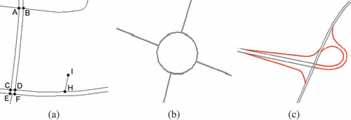
Figure 1. Dual carriageways: for example parallel lines A→C→E and B→D→F in (a); narrow passages: for example road A→B in (a); navigation stubbles: for example road H→I in (a); roundabouts in (b); slip roads around cloverleaf junctions in (c).

2.1. Structure recognition

In this process, six different types of ‘structures’ can be identified, namely

• roundabouts (looping crosses)

• dual carriageways (parallel roads)

• slip roads around cloverleaf junctions

• narrow passages

• navigation stubbles

• normal single carriageways

2.1.1. Recognition of roundabouts

The roundabouts (looping crosses) can be detected by comparing the coordinate pairs of a polyline: at first a sequence of line objects sharing certain characteristics (e.g. the principle of ‘good continuity’ in Gestalt psychology) is chained to form a polyline. If two points along the chain claim the same geometric position, they indicate the existence of a roundabout.

2.1.2. Recognition of the dual carriageways (parallel roads)

The automatic recognition of parallel roads is more perplexed, which starts with an exploring procedure in the datasets: if two closely located polylines reveal similar geometric properties, including angular, length and maximal chord, and do not intersect, they will be associated with parallel roads and treated as one item. To facilitate the subsequent matching approach, each of the anticipated parallel lines should be delimited by the intersection (valence ≥ 3) or ending node (valence = 1) of a road. It should be noted that if the exploring procedure has to traverse all road objects, it will unnecessarily consume too much computing time because (a) the recognition of parallel roads is computing intensive and (b) most of the matching references do not belong to the special cases of parallel roads. For these reasons, the recognition process is triggered only under some conditions, for example when polylines are short (<30 m) and have their ending nodes with the valence of 3 or 4. The narrow passage roads A→B, C→D, E→F, C→E and D→F in Figure 1a are such polylines.

2.1.3. Recognition of the slip roads around cloverleaf junctions

Recognition of the slip roads is one of the most complex tasks in our proposed matching approach. It takes place after the recognition of the dual carriageways and can be characterized by two steps: (1) detection of the cloverleaf junctions: a sequence of adjacent intersections crossed by dual carriageways can be regarded as cloverleaf junctions and (2) identification of the slip roads: a single carriageway, which is near to the cloverleaf as well as connected to dual carriageways, will be recognized as a slip road. It has to be noted that the recognition of the slip roads depending only on the geometrical characteristics could be very hard in some cases. To enhance the computing efficiency, the semantic information should be considered.

2.1.4. Recognition of the narrow passages and navigation stubbles

The narrow passages and navigation stubbles can be rather easily identified by the lengths and the topological characteristic of the ending nodes: a narrow passage is a short road (e.g. <100 m) with both ending nodes delimited by intersections; whereas a short road delimited by an intersection and a dead end is regarded as navigation stubble.

2.1.5. Normal single carriageways

The remaining line objects that do not belong to any of the structures recognized in Sections 2.1.1–2.1.4 are treated as normal single carriageways in the further matching processes.

2.2. Process modelling

Structure recognition is followed by process modelling, which assigns different matching algorithms as well as the necessary criteria to differentiate structure categories. In this section, the authors will particularly demonstrate the matching strategies for two challenging cases that have not been widely investigated so far – dual carriageways (parallel lines) and looping crosses as illustrated in Figure 1a and b.

2.2.1. Matching of single carriageways

As slip roads, narrow passages, navigation stubbles and the normal single carriageways are single polylines, their matching processes are similar. For the matching of single polylines, two of the most popular and well-known matching algorithms reported in literature – buffer growing (BG) (Walter and Fritsch 1999, Mantel and Lipeck 2004, Zhang and Meng 2007) and iterative closest point (ICP) (Besl and McKay 1992, Gösseln and Sester 2004, Volz 2006) are available. So far a majority of the developed matching approaches based on BG, ICP or combination of them have revealed a high matching rate and efficiency on certain data types of selected test areas. Moreover, it has been generally assumed that a better matching result can be reached with more context information (Mustière 2006, Stigmar 2006). Based on this commonsense assumption, a matching algorithm, namely delimited-stroke-oriented (DSO) algorithm, has been developed to achieve the more robust and generic matching between different road networks (Zhang and Meng 2008). The experiments conducted in Zhang and Meng (2008) have confirmed the considerably improved matching performance of the DSO algorithm in terms of computing speed, matching rate, matching certainty and robustness. Because of its ‘robustness’ and ‘generic’ nature, the DSO algorithm has been employed in this process to match the corresponding single polylines between two comparable datasets, including slip roads, narrow passages, navigation stubbles and normal single carriageways.

The roundabouts (looping crosses) or dual carriageways (parallel lines), however, take on quite different geometric or topologic characteristics from the single carriageways. Therefore, it is inappropriate to directly employ the DSO matching algorithm, that is further matching strategies are necessary to deal with these two challenging cases. Worth mentioning is that the proposed matching strategy can handle the dual carriageways or roundabouts with both similar and distinctive LoDs.

2.2.2. Matching of the roundabouts

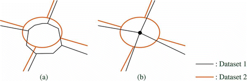
The following two-step matching process can be utilized to identify the corresponding roundabouts between different datasets with: (a) the corresponding roundabouts with similar LoDs, see the two polygons in Figure 2a; and (b) the corresponding roundabouts with different LoDs, for example in Figure 2b one road roundabout is represented by a loop in one dataset whereas it is just a node in the other.

Figure 2. Corresponding roundabouts with (a) similar or (b) dissimilar LoDs.

Step 1:

Matching the roundabouts with similar LoDs

As depicted in Figure 2a, the corresponding roundabouts with similar LoDs are often represented by two polygons in different datasets. The correspondence between homologous polygons can be identified by comparing their geometric characteristics with respect to the area, location and shape.

• Area difference Comparing the areas (S) between two polygons from different datasets helps to judge whether these two polygons are corresponding roundabouts or not, see the normalized area difference in Equation (1)(1):

  (1)

  Knowing that PL_g1 and PL_g2 represent the roundabouts to be compared, and are predefined maximal and minimal tolerance values of the area difference between corresponding polygons and is a predefined tolerant ratio divided by the area difference and summation.

• Location difference The distance between the centre points of the roundabouts to be compared can be utilized to measure their location difference in the matching process. This distance can be normalized by N(d _PLg) in Equation (2)(2), where the d _PLg represents the distance between two centre points and the tolerance value is given empirically:

  (2)

  The location difference is a significant parameter for the detection of possible corresponding roundabouts between different datasets.

• Shape difference The shape of a polygon can be roughly represented by two variables R _L‐PLg and σ_r‐PLg defined in Equations (3)(3) and (4):

  (3)
  where l _L represents the length of the longest chord and S _PLg the area of the polygon and
  (4)
  where r_i is the distance between the centre point and the vertex of a polygon and is the average value.

In the proposed matching model, the shape difference between two polygons PLg₁and PLg₂ can be measured by the normalized values of R _L‐PLgand σ_r‐PLg defined in Equations (5)(5) and (6). Knowing that , , , , and are predefined thresholds with respect to the tolerant differences between the corresponding polygons from different datasets, hereinto , , and are in metric space, whereas and are ratios:

(5)

(6)

Based on the characteristics of size (area), location and shape, the exclusion criteria for the roundabouts matching can be defined as

(7)

where and is a standard unit vector. The roundabout PLg₁ and PLg₂ are confirmed as promising correspondences if they pass the exclusion criteria in Expression (7); otherwise they will be rejected as wrong matching suggestions.

In case that the reference roundabout PLg₁ has more than one corresponding roundabout in the target dataset which passes the exclusion criteria of , interpreted as , none of the can be simultaneously regarded as correct counterpart to PLg₁. Two options are available for the confirmation of a unique matching counterpart. One is to weigh the different criteria according to their relative contributions: the matching pair constituted by PLg₁ and with the largest value of weighted sum is regarded as the best matching, whereas all the others are discarded. The weighted sum of measurements can be calculated by

(8)

where is a weight vector given empirically by the user; and . The other option is to stepwise decrease the tolerance value in Equations (1)(1), (2)(2), (5)(5) and (6)(6), until only one matching pair remains.

Step 2:

Matching of the roundabouts at different LoDs

The same real-world roundabout could have very different representations in different datasets, for example the roundabout depicted in Figure 3a appears as a loop crossing in Dataset 1 (see polygon in Figure 3b), whereas in the Dataset 2 at a coarser LoD it is generalized as a node (see node A′ in Figure 3c). In this case, matching the corresponding roundabouts has become a task to identify the correspondence between a polygon and a node. As polygon and node reveal distinct geometric and topologic characteristics, it is impossible to measure their similarities in a straightforward way. Bearing this artefact in mind, the authors propose a devious matching strategy which can be elucidated by the example in Figure 3.

Figure 3. Matching roundabouts at different LoDs: overlapping of two LoDs (a) from Dataset 1, (b) and Dataset 2 (c).

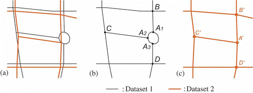
In Figure 3, the polygon from Dataset 1 is selected as the ‘reference’. In the aforementioned matching Step 1, no corresponding polygon in Dataset 2 can be identified as the counterpart of the ‘reference’ as the roundabout is represented too differently in these two datasets. Therefore, the matching process between polygon and node is triggered. The branches connected to the polygon and the node are compared. As depicted in Figure 3b, the ‘reference’ polygon has three branches, viz. , and , which can be interpreted as , where n represents the valence of the roundabout and all the are polylines. Subsequently, the matching process is conducted for each in turn. The matching result is recorded in a set of , where CP _i represents the counterpart of Branch _i in Dataset 2.

If the matching process has successfully identified the counterpart for Branch _i , the CP _i in Dataset 2 is denoted as , otherwise the CP _i is a null set denoted as φ. Two alternative strategies are possible to identify the correspondence between the polygon and node.

Strict strategy:

If every Branch _i of the ‘reference’ polygon PLg in Dataset 1 can find its counterpart in Dataset 2, namely , and all polylines in intersect at a node A′, then the polygon PLg and node A′ will be matched together.

Loose strategy:

In case that not every Branch _i of the reference polygon PLg in Dataset 1 can find its counterpart in Dataset 2, the set of can be divided into two parts, namely and . The polygon PLg and node A′ will be confirmed as counterparts if (a) the dimension (size) of is much smaller than that of ; and (b) the node A′ is shared by all polylines in set .

The matching strategy with looser criteria can lead to a higher matching rate (completeness) than the strict strategy, whereas the strict strategy often reveals a higher matching certainty.

2.2.3. Matching of dual carriageways

Similar to the classification of roundabouts, the corresponding dual carriageways can be also categorized into two groups according to their representations:

1. The corresponding dual carriageways reveal similar LoDs, that is they are represented by two pairs of parallel lines (one for each direction) in both datasets.

2. The dual carriageways reveal different LoDs, for example a road is a single polyline in one dataset, whereas it is represented by dual carriageways, that is a pair of parallel lines in the other dataset.

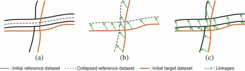
The DSO matching algorithm mentioned in Section 2.2.1 can hardly deal with dual carriageways, especially when they are represented in different LoDs in the datasets to be compared. One efficient way to solve this problem is to embed a generalization process of the dual carriageways to the overall matching approach. At first, the dual carriageways in the datasets to be matched are recognized and generalized (collapsed) to their centre lines. The subsequent matching process is then conducted on the centre lines. After the matching, however, the original dual carriageways will replace these temporary centre lines to generate the ultimate matching results. The detailed matching process can be characterized by the following three steps.

Step 1:

Collapsing of the dual carriageways

Once the dual carriageways (line pairs) are recognized, their centre lines can be derived. In the context of road-network matching, the collapse procedure has to meet the following requirements: (a) the neighbouring features, namely the roads connecting to the initial dual carriageways, need to be adjusted so that no gaps and no overlaps occur; (b) the topologic relations between the dual carriageways and neighbours need to be preserved; and (c) the neighbours should be modified as little as possible. To satisfy all three requirements, the authors have proposed the following collapsing method.

First, the ‘node pairs’ are detected. Two closely located nodes which lie on different sides of the recognized dual carriageways and share certain topologic characteristics can be treated as a ‘node pair’. In this step, there are four types of ‘node pairs’ in total, see examples in Table 1 where the ‘node pair’ is denoted as (N ₁, N ₂). Types (a)–(c) can be easily detected as they are connected by narrow passages, whereas the detection of type (d) needs a comparison of their topologic characteristics.

Table 1. Different types of ‘node pairs’

Example
Type	(a)	(b)	(c)	(d)

Second, with the identified ‘node pairs’ as terminating points, the whole dual carriageway can be split into smaller sections, see the example in Figure 4a and b. Each section is constituted by two parallel polylines, denoted as , where and are represented by two chains of oriented vertices, namely and . By means of interpolation, each vertices of can find its corresponding position along , denoted as , where and . Likewise, the corresponding position of on , can be also identified, denoted as . Subsequently, the vertices of and are aligned to the centre points represented by and . Following a proper sequence, all of the points and can be chained together and act as the collapsed centre line of the divided section , denoted as , see the example of thick grey lines in Figure 4b.

Figure 4. An example of collapsing dual carriageways.

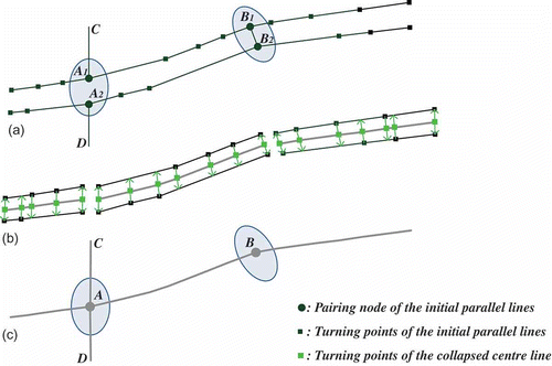
By connecting all the together, we get the collapsed centre lines of the dual carriageways, see example in Figure 4c. Along with the collapsing operation, the neighbours of the dual carriageways are also transformed based on the displacement vectors of and , for example the neighbouring roads and in Figure 4a have been, respectively, extended to and in Figure 4c, whereas the narrow passage is replaced by the node B.

Step 2:

Matching of the dual carriageways with similar LoDs

After collapsing of the dual carriageways, two pairs of temporal files are established to record the collapsed dual carriageways from the reference and target dataset: one is constituted by where and represent the initial and collapsed dual carriageways from the reference dataset, respectively, interpreted as ; and the other is the pair of and , where , and .

To identify the corresponding dual carriageways with similar LoDs between different datasets, the matching process is conducted between the sets of and , where and act as the basic items for the matching. As a generic case of matching, the polyline chained by from the reference dataset could be matched to the polyline from the target dataset. As the ultimate matching result, the and is replaced by the initial dual carriageways of and , which will result in two matched pairs of polylines, namely

1. and ;

2. and ,

where , , and the polygon enclosed by and has a consistent orientation to that of and , for example, both of them are counter-clockwise.

Step 3:

Matching of the dual carriageways with dissimilar LoDs

This step deals with the dual carriageways that cannot find their counterparts with similar LoDs in the other dataset. After Step 2, the unmatched dual carriageways from the reference dataset are denoted as and where and represent the initial and collapsed dual carriageway from the reference dataset, respectively, namely ; and unmatched dual carriageways from the target dataset are denoted as and , where , and .

To deal with the unmatched dual carriageways from the reference dataset, the matching process is triggered to calculate the corresponding single polylines between from the reference dataset and the entire target dataset. As an example of successful matching, the polylines and PL_tag could be identified as temporal counterparts between different datasets, where is chained by various from and PL_tag is constituted by original road objects from the target dataset. Replacing by , the becomes two parallel lines, which can result in an equivalent matching pair between different datasets, that is a pair of dual carriageways from reference dataset have been successfully matched to a single carriageway from the target dataset, see the example from Figure 5a–c. Likewise, the matching process can be conducted between from target dataset and the entire reference dataset.

Figure 5. Matching of the dual carriageways with dissimilar LoDs.

2.3. Process execution

Process execution as the final step takes place to operate the matching approach. As known, different structure categories have different matching processes. To get desirable results these matching processes have to be integrated together. Considering that the structures of dual carriageways, roundabouts, narrow passages, navigation stubbles and slip roads are holding several particular characteristics, their matching processes will be triggered ahead of the normal single carriageways in the integrated matching approach. However, if a structure among dual carriageways, narrow passages, navigation stubbles or slip roads from the reference dataset cannot find its corresponding structures from the target dataset, it will be treated as normal single carriageways hereafter and then go through the normal matching process.

3. Experiments

3.1. Test data

The conducted matching experiments involve four different datasets:

ATKIS

It was captured through map digitization in combination with semiautomatic object extraction from imagery data. The data structure is defined in accordance with the Official Topographic Cartographic Information System. The road layer of ATKIS is composed of geometries and general-purposed attributes of road lines. Each captured road is displayed in the cartographic database as a line representing the centre line of the road (AdV 2003). However, the attributes are not completely covered with values, especially the street names which are essential clues for the matching are only sporadically available.

Tele Atlas

It is a fully attributed dataset containing detailed road network, water features, parks and landmarks, etc. The Tele Atlas road network contains geometries and navigation-oriented attributes of road lines (middle axes) which were captured through map digitization, GPS-supported field measurement and dynamic supervision of traffic information. In Europe, it has an absolute accuracy of within 10 m inside built-up areas and 25 m outside built-up areas. In dense urban areas where up-to-date source material is present, an accuracy of a few meters can be expected.

NAVTEQ

It is a world leader in the creation, maintenance and distribution of digital navigable maps. Similar to Tele Atlas, the NAVTEQ road network contains geometries and navigational attributes of road lines (middle axes), which were captured through map digitization, GPS-supported field measurement and dynamic supervision of traffic information. Every single road object can be described with more than 160 attributes such as street names, access limitations, time and turn restrictions and speed limits, which allow, for example, a vast variety of different applications on fleet operations and location-based services (LBS).

OpenStreetMap (OSM, http://www.openstreetmap.org)

It is a collaborative project to create and provide free geographic data such as street maps of the world based on Web 2.0. The initial OSM map data were built from scratch by volunteers performing systematic ground surveys using handheld GPS devices. More recently, the availability of aerial photography and other data sources has greatly increased the speed of this work, thus allowing land-use data to be collected more accurately (Wikipedia 2009).

3.2. Matching performance

The proposed structure-guided matching approach has been successfully implemented to match different road networks among (1) ATKIS, (2) Tele Atlas, (3) NAVTEQ and (4) OSM; the selected test areas cover a number of federal states in Germany, such as Berlin, Hessen, Lower Saxony and Bavaria, containing coastal and inland areas, mountainous and flat areas, rural and built-up areas. After comparing the automatic matching results with the manually corrected ones, the performance of the proposed matching approach is evaluated. Table 2 shows the statistical matching results of four typical test areas which are selected randomly.

Table 2. The statistical matching results and computing efficiency

	Matching between
Number.	Dataset A	Dataset B	Matching area	Matching rate	Matching correctness	Computing time (seconds)
1	10,947 objects (ATKIS)	10,360 objects (Tele Atlas)	ca. 1200 km^2	97.2%	99.1%	22
2	2214 objects (NAVTEQ)	5011 objects (ATKIS)	ca. 120 km^2	95.8%	99.1%	6
3	1762 objects (ATKIS)	571 objects (NAVTEQ)	ca. 100 km^2	94.7%	99.7%	2
4	4226 objects (OSM)	3122 objects (NAVTEQ)	ca. 40 km^2	97.8%	98.8%	4
Configuration of the computer			Intel Centrino Core Duo 2.0 GHz, 2G physical memory

To further assess the performance of the proposed matching approach, a few detailed matching cases are discussed below.

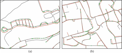
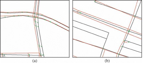
Figure 6 shows some efficient cases for the street matching between ATKIS and NAVTEQ. In these cases, the contextual matching approach reveals a perfect matching completeness and accuracy: not only the lines but also the nodes are accurately matched through the comparison of the topologic connection between nodes and lines.

Figure 6. Two efficient matching cases. Dark grey lines: ATKIS; light grey lines: NAVTEQ; arrows: linkages.

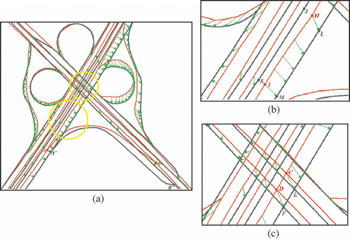
Being aided by the structure-guided matching strategy, the proposed approach has revealed high matching rate and accuracy for loops, parallel roads and even complex crossings, for example Figure 7 shows an efficient matching case for looping crosses; and Figure 8 illustrates the complex matching cases around highways. In Figure 8, the dual carriageways and some other slip roads are accurately matched between different datasets. As the parallel roads are treated as one item, the contextual matching approach does not necessarily match the closest objects together, for example the Tele Atlas road shown in Figure 8b has two candidates in ATKIS – road and , and is matched to the farther one – road . As the structure-guided matching takes the holistic sequence of the nodes into consideration, the node matching proves efficient around the cloverleaf junction, such as node and in Figure 8c, where the topologic connections are very complex.

Figure 7. Efficient matching cases for looping crosses. Dark grey lines: OSM, light grey lines: NAVTEQ; arrows: linkages.

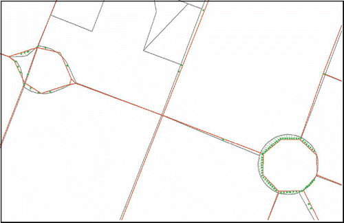
Figure 8. A complex matching case around highways. Dark grey lines: ATKIS; light grey lines: Tele Atlas; arrows: linkages.

Particularly, the proposed matching approach can be also employed to match the streets at very different LoDs as the generalization process has been integrated to the matching calculations. Figure 9, for example, shows two matching cases which take place on the dual carriageways between the datasets of OpenStreetMap (OSM) and NAVTEQ, where the dual carriageways are represented by parallel lines in one dataset and single polylines in the other. Still they are properly matched together by the proposed matching approach.

Figure 9. Matching of the dual carriageways at different LoDs. Dark grey lines: OSM; light grey lines: NAVTEQ; arrows: linkages.

Nevertheless, the matching results are not always perfect. The node B on the lower right corner of Figure 8a, for example, should be matched to the node B′ from the topological point of view. Unfortunately, these two corresponding nodes were not matched together because they have been placed too far from each other (about 100 m). This kind of problem often occurs, especially when the datasets to be matched reveal a substantial discrepancy in data accuracy.

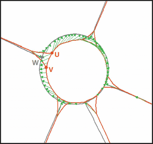
Furthermore, the topologic ambiguities can influence the matching performance as well, for example in Figure 10, the ATKIS node W has two corresponding nodes U and V in Tele Atlas. Ideally, the node W should be matched neither to U nor to V but to the centre point of them. However, this occasion has not yet been considered in the current matching approach. In addition, the proposed matching algorithm may also suffer some limitations if the topologic contexts are very inconsistent or if the objects in the dataset are highly fragmentary.

Figure 10. Ambiguous corresponding nodes between ATKIS and Tele Atlas. Dark grey lines: ATKIS; light grey lines: Tele Atlas; arrows: linkages.

4. Conclusions

This article is devoted to a structure-guided approach for the automatic road-network matching. The approach is constituted by three hierarchical processes of ‘category recognition’, ‘process modelling’ and ‘process execution’; and touches upon not only the common single carriageways but also the challenging cases of the slip roads, roundabouts, dual carriageways (parallel lines), etc. Being supported by certain generalization operators, the ‘structure’-guided matching approach is able to correlate the counterparts from different datasets at either similar or dissimilar LoDs.

Taking advantages of classifying the road network into several structure categories and then developing a category-sensitive matching strategy with proper parameters or criteria for each category, the proposed matching approach has yielded a considerably improved performance in terms of the following:

1. Automatic matching reliability and accuracy: In a number of large test areas in Germany, the overall matching rate exceeds 97%; among the matched objects more than 99% are correct. With less than 3% unmatched objects and 1% matching errors in spite of data complexity and ambiguity, the proposed structure-guided matching approach is highly successful. We believe that holistically perfect matching approaches are possible only if the context information can be adequately considered (Zhang and Meng 2007).

2. Generic nature: The proposed matching approach does not necessarily rely on any semantic information, therefore, it can work with the worst case – one or both of the datasets to be matched have no or little semantic information (e.g. ATKIS and OSM data). The gained insight from road-network matching can therefore be easily adapted to the task of matching other linear features such as electronic or hydrological networks.

3. High computing speed: For example, in a test region of approximately 1200 km², there are 10,959 ATKIS objects and 10,681 Tele Atlas objects. The matching has taken only 22 seconds in a normal PC (personal computer), that is about 500 objects per second (Table 2). This computational effectiveness has much to do with the employment of the grid-based spatial indexes for points and lines introduced in Zhang et al. (2009). Moreover, with the use of the grid-based spatial indexes, the matching speed can approximately keep stable along with an increasing network size (Schimandl et al. 2009).

Worth mentioning is that the proposed road-network matching approach has been successfully implemented for the real-world navigational data enrichment for whole Germany and is being tested for many other European countries and metroregions (United Maps 2010). The positive automatic matching performance and the successful applications in the real-world project demonstrate that the proposed matching approach has the substantial potential for the commercialization.

Acknowledgements

The research described in this article is co-sponsored by Federal Agency for Cartography and Geodesy, Corp. United Maps and Technische Universität München.

References

- 2003 . AdV, Arbeitsgemeinschaft der Vermessungsverwaltungen der Länder der Bundesrepublik Deutschland , Amtliches Topographisch- Kartographisches Informationssystem ATKIS . 2003
- Besl , P. and McKay , N. 1992 . A method for registration of 3-d shapes . IEEE Transactions on Pattern Analysis and Machine Intelligence , 14 ( 2 ) : 239 – 256 .
- Devogele , T. , Parent , C. and Spaccapietra , S. 1998 . On spatial database integration . International Journal of Geographical Information Science , 12 ( 4 ) : 335 – 352 .
- Gabay , Y. and Doytsher , Y. Automatic adjustment of line maps . Proceedings of GIS/LIS’94 Annual Convention. American Congress on Surveying and Mapping, American Society for Photogrammetry and Remote Sensing, Association of American Geographers, Urban and Regional Information Systems Association, and AM/FM International . Phoenix, Arizona. pp. 333 – 341 .
- Gabay , Y. and Doytsher , Y. 1995 . Automatic feature correction in merging of line maps . Proceedings of the 1995 ACSM-ASPRS Annual Convention , 2 : 404 – 410 .
- Gösseln , Gv and Sester , M. Integration of geoscientific data sets and the German digital map using a matching approach . XXth ISPRS Congress . July 12–23 2004 , Istanbul, Turkey. pp. 1249 – 1254 .
- Mantel , D. and Lipeck , U. Matching cartographic objects in spatial databases . XXXV ISPRS Congress . July 2004 , Istanbul, Turkey. pp. 12 – 23 . Commission 4
- Mustière , S. Results of experiments of automated matching of networks at different scales . XXXVI ISPRS Workshop – multiple representation and interoperability of spatial data . February 2006 , Hannover, Germany. pp. 22 – 24 .
- Mustière , S. and Devogele , T. 2008 . Matching networks with different levels of detail . GeoInformatica , 12 : 435 – 453 .
- Raimond , A.-M.O. and Mustière , S. 2008 . “ Data matching – a matter of belief, headway in spatial data handling ” . In 13th International symposium on spatial data handling (SDH) , 501 – 519 . Montpellier : Springer . 2008
- Schimandl , F. Real time application for traffic state estimation based on large sets of floating car data . International scientific conference on mobility and transport – ITS for larger Cities . May 2009 , Munich, Germany. pp. 12 – 13 .
- Stigmar , H. 2006 . Some aspects of mobile map services. Licentiate Dissertation , 1652 – 4810 . Sweden : Lund University . ISSN
- United Maps, 2010. http://www.unitedmaps.net/ (http://www.unitedmaps.net/) (Accessed: 28 January 2010 ).
- Volz , S. An iterative approach for matching multiple representations of street data . XXXVI ISPRS Workshop – multiple representation and interoperability of spatial data . February 2006 , Hannover, Germany. Edited by: Hampe , M. , Sester , M. and Harrie , L. pp. 22 – 24 .
- Walter , V. 1997 . Zuordnung von raumbezogenen Daten – am Beispiel der Datenmodelle ATKIS und GDF , Dissertation, Deutsche Geodätische Kommission (DGK) Reihe C, Nummer 480 .
- Walter , V. and Fritsch , D. 1999 . Matching spatial data sets: a statistical approach . International Journal of Geographical Information Science , 13 ( 5 ) : 445 – 473 .
- Wikipedia, 2009. http://en.wikipedia.org/wiki/OpenStreetMap (http://en.wikipedia.org/wiki/OpenStreetMap) (Accessed: 2 October 2009 ).
- Yuan , S. and Tao , C. Development of conflation components . Proceedings of Geoinformatics’99 . June 1–13 1999 , Ann Arbor. pp. 19 – 21 .
- Zhang , M. A grid-based spatial index for matching between moving vehicles and road-network in a real-time environment . Proceedings of the XXIVth international cartographic conference (ICC) . November 2009 , Santiago, Chile. pp. 15 – 21 .
- Zhang , M. and Meng , L. 2007 . An iterative road-matching approach for the integration of postal data . Computers, Environment and Urban Systems , 31 ( 5 ) : 598 – 616 .
- Zhang , M. and Meng , L. 2008 . Delimited stroke oriented algorithm – working principle and implementation for the matching of road networks . Journal of Geographic Information Sciences , 14 ( 1 ) : 44 – 53 .