Distributed LiDAR data processing in a high-memory cloud-computing environment

Abstract

This article explores the use of an advanced, high-memory cloud-computing environment to process large-scale topographic light detection and ranging (LiDAR) data. The new processing techniques presented herein for LiDAR point clouds intelligently filter and triangulate a data set to produce an accurate digital elevation model. Ample amounts of random-access memory (RAM) allow the employment of efficient hashing techniques for spatial data management; such techniques were utilized to reduce data distribution overhead and local search time during data reduction. Triangulation of the reduced, distributed data set was performed using a local streaming approach to optimize processor utilization. Computational experiments used Amazon Web Services Elastic Compute Cloud resources. Analysis was performed to determine (1) the accuracy of the binning/array-based reduction, as measured by root mean square error and (2) the scalability of the approach on varying-size clusters of high-memory instances (nodes having 244 GB of RAM). For experimental data sets, topographic LiDAR data generated by the Iowa LiDAR Mapping Project was used. This article concludes that the data-reduction strategy is computationally efficient and outperforms a comparable randomized filter control when moderate reduction is undertaken – e.g., when the data set is being reduced by between 30% and 70%. Performance speed-up ratios of up to 3.4, comparing between a single machine and a 9-node cluster, are exhibited. A task-specific stratification of the results of this work demonstrates Amdahl’s law and suggests the evaluation of distributed databases for geospatial data.

Keywords:

• LiDAR
• cloud computing
• spatial data
• data reduction
• triangulation

1. Introduction

1.1. Overview

Recent advances in remote sensing and imaging technology have made possible the routine generation of massive spatial data sets. Making best use of state-of-the-art computing resources to keep pace with the rapid growth in spatial data set sizes is an important challenge in geographic information system (GIS) (Yang and Huang 2013). Today, next-generation cloud-computing clusters are being designed with rapidly increasing amounts of random-access memory (RAM) per node (128 GB to 2 TB or more). Moreover, current advanced high-performance computing (HPC) resources may have an order of magnitude more CPU cores than a typical HPC machine of 5 years ago, while possessing only limited improvements in the sequential processing capabilities of a single processor core. These changes in the HPC landscape provide both opportunities and challenges for big spatial data computing.

Three-dimensional spatial imaging with light detection and ranging (LiDAR) technology is a powerful remote sensing methodology that can be used to produce detailed maps of objects, surfaces, and terrain across widely varying scales. As scanning technology has continued to improve, massive high-density LiDAR point clouds have become easier to generate, and the creation of accurate, compact terrain models and other three-dimensional representations has therefore assumed greater prominence. However, the generation of such improved models from increasingly voluminous data sets poses significant challenges in data processing and demands commensurate increases in computing power. This article develops and implements new techniques for processing large LiDAR point clouds that harness recent improvements in HPC technology. The new processing techniques presented herein intelligently filter and triangulate input data sets to produce an accurate digital elevation model (DEM). Importantly, advantage is taken of large memories, data locality, and hashing (array lookup) to generate a time-space trade-off.

1.2. Related work

1.2.1. Approaches to data reduction

As in other domains, improvements in data-collection technology have allowed the production of massive quantities of data (hence the term big data) that pose challenges for data-processing techniques. Data is only valuable in its ability to convey information, and not all data in a large LiDAR point cloud supplies an equal amount of information about the source terrain. For a DEM to be useful, it must be of an appropriate size to be manipulable by whatever technology is being used to display it. These issues thus define a central challenge in large-scale geospatial data processing – how to reduce data in accordance with the data set size requirements of a domain while maintaining optimal per-size resolution.

A variety of methods and ideas have been developed to reduce data set size while retaining information (Anderson, Thompson, and Austin 2005; Krishnan, Baru, and Crosby 2010; Oryspayev et al. 2012). In terms of data set size reduction, two techniques are generally used. The first is decimation, or the selective removal of particular points thought to convey little information, from the LiDAR point cloud (e.g., Oryspayev et al. 2012). The second is gridding, in which the entire point cloud is replaced by a rasterized image created using an interpolation method to generate an approximate z-value for each grid point (e.g., Krishnan, Baru, and Crosby 2010).

1.2.2. Approaches to triangulation

Digital terrain models (DTMs) are generally used to represent topographic data in GIS. The two main data formats used for DTMs are raster format (in which the landscape is decomposed into uniform cells) and triangulated irregular network (TIN) format. In a TIN model, points are connected by line segments to form triangles; such triangles provide a continuous, faceted representation of the terrain surface. In triangulating a surface, a certain extremal triangulation, the Delaunay triangulation (DT), is preferred for its rigorous structural properties (Peucker et al. 1978). By default, a triangulation of a surface should be a Delaunay, or near-Delaunay, triangulation.

Various algorithms have been developed to calculate the DT for a given set of (x,y) points in the plane; these include the incremental approach (Lawson 1977; Watson 1981), as well as algorithms that use the plane sweep and divide and conquer paradigms (cf. Dwyer 1987; De Berg et al. 2000). Theoretically, the time complexity of an efficient sequential algorithm for DT is O(n log n) (Dwyer 1987). In practice, if a TIN is desired for a very large number of data points collected by LiDAR, it may take hours to generate using a traditional sequential hardware/software system. One approach to speeding up this operation is to make use of multiple processors. The parallelization of DT has been studied by many researchers (see Kohout, Kolingerová, and Žára 2005). Isenburg et al. (2006) proposed an algorithm that performs the computation in a streaming fashion; the algorithm processes the data as it reads and uses a point insertion algorithm for triangulation. Wu, Guan, and Gong (2011) extended this approach for multicore architectures. Lo (2012) suggested that data points be partitioned into overlapping zones. In this course-grained approach, a processor is then assigned to each zone to compute its DT in a sequential manner.

The algorithms discussed earlier assume access to a shared memory. Also, the parallelization is local rather than distributed, that is, all of the multiple processors reside on a single machine and have access to the shared memory.

Recent advances in cloud-computing services have made it easier to access distributed computing environments. Such environments provide users with considerable processing power and a distributed memory capacity, presenting opportunities to improve performance. This motivates the study of parallel computation of the DT in a distributed-computing environment. In this work, a distributed framework for processing massive amounts of LiDAR data was designed and implemented, and this implementation was tested using the Amazon Web Services Elastic Compute Cloud (EC2) infrastructure. LiDAR data sets were processed in sizes from 12 to 95 GB.

1.2.3. Approaches to distributed processing of spatial data

Although the historical trend known as Moore’s law has seen the continued evolution of ever-faster processors and ever-larger memories, the rate of improvements in processing power has slowed recently, and physical limitations such as power consumption and heat dissipation are becoming increasingly important. As well, data-driven application domains are experiencing data growth that is unmatched by processing power, due to these physical limitations. As a consequence, at the scales of new massive spatial data, a single thread of execution on a single CPU is simply not satisfactory from the perspective of processing time.

1.2.4. Cloud computing and Amazon EC2

Within the past decade, cloud computing and other HPC systems have become available to the average researcher and consumer under pay-per-use schemes (Barr 2006). The concept behind cloud computing is the idea of offering computing as a service – customers have an ever-more-diverse set of needs and computational products they desire and often wish to be able to customize their computing systems at a fairly low level. Prior to cloud computing, software products generally assumed either (1) end-user ownership of hardware or (2) fairly rigid domain specificities. With cloud computing, the idea is to provide managed computational resources as a commercial product, letting the end-user choose and deploy software on top of underlying, seamless, hardware/network/operating system layers. The advent of commercialized cloud-computing systems has allowed individuals and small organizations access to previously unavailable computing power. Amazon’s EC2 (AWS 2014) is a leader in the industry, although other providers (Google, Microsoft) have also deployed pay-as-you-go cloud platforms. Amazon EC2 was employed for this research due to the availability of particular processor/memory/operating system architectures, including 16-core nodes with 244-GB memories and solid-state storage.

1.3. Contributions

This work develops and explores several new ideas related to LiDAR data reduction and processing; experiments are performed with LiDAR processing of a scale that has previously seen little attention in the literature.

1.3.1. Binning reduction with high memory

As part of the new approach, the standard computational technique of hashing was applied in a straightforward manner to LiDAR data processing to take advantage of a time-space trade-off. By allocating sufficient memory to divide the physical region into many small logical bins such that the average point density is on the order of one point per bin, typical logarithmic search overheads can be replaced by array-lookup operations when it comes to the common task of determining which data points are physically near to the point under consideration. It is important to note that this approach is computationally efficient due to the broadly uniform distribution of data points in the (x,y) plane in most LiDAR data sets derived from real-world topography.

1.3.2. Physically Ordered Delaunay triangulation

The in-memory data structure utilized also allowed the adaptation of an already practical implementation of DT (Sloan 1987) for additional efficiency. In particular, one of the time costs that arises in this algorithm (which is otherwise of optimal efficiency) is the number of comparisons required to determine the existing triangle containing the point under consideration. When the current point under consideration is physically close to recently added points, this cost is reduced. By using the binned data structure, points can be added to the triangulation in an order that encourages a small number of required comparisons; by inserting points in a ‘locally sequential’ manner, the number of comparisons required to locate the new point in the existing triangulation is reduced.

1.3.3. Optimizations

The size of the large experimental data set (95 GB) is of a scale that has seen little attention in prior work. One of the purposes of this work was to explore the practicality of reducing and triangulating LiDAR data sets of this scale. After some technical effort, a software solution was produced that was able to reduce the Johnson County, Iowa data set by a third and triangulate it, achieving a small root mean square error (RMSE), in 37 minutes (see Section 4). This demonstrated that commodity, or near-commodity, networks are sufficient to support the distributed processing of large-scale LiDAR data sets – though this demonstration came only after the implementation of appropriate network buffering in the processing software.

2. High-level methodology

Several questions drove the selection of techniques and algorithms: (1) Can large, distributed quantities of RAM be used to allow the reduction and triangulation of previously unstudied LiDAR data set sizes, in reasonable timeframes? (ii) Is a linear speed-up achievable for a distributed approach to LiDAR data processing in memory? (iii) Can vertex decimation be done accurately prior to triangulation?

With regard to question 1, the reduction and triangulation of a LiDAR point cloud can, in theory, be considered a high-throughput computing (HTC) problem due to the general principle of (geometric) locality in spatial data sets. That is, in building a terrain model, any particular portion of the model can be constructed using only data from the point cloud in a neighbourhood of that portion. Data-processing models that fall into the HTC category are generally attractive because they may often be turned into streaming-type algorithms that need only see a particular data point once and need only maintain it in memory for a finite period of time (thus obviating large memory requirements) to accomplish the desired task.

2.1. Data reduction and triangulation

2.1.1. Utilization of large memories

Fitting an algorithm for spatial data processing into the HTC model is highly dependent on the locality of the format of the input. That is, data points that are close to each other in space should also be close in the input filestream. This is not always possible, even if the input data were presented according to a space-filling curve. It is therefore necessary in the reduction and triangulation of spatial data to revisit data that may have been first used some time ago. If the data set is large, this may require input from a mass storage device, which is often one of the slowest components of any system. The necessity of using and reusing any particular data point over the lifetime of a process naturally leads to a desire to be able to store the entire input in fast (volatile) storage, such as RAM. Advances in technology over the past decade have made it possible for individual servers to possess as much RAM today as might have existed in an entire cluster a decade ago: 256 GB, 512 GB, or more. In industry, high-use, moderate-size databases that were once stored on disk are often being moved entirely into main memory, dramatically improving access times.

To take advantage of large quantities of RAM on each node, a data structure was created in memory using a binning/hashing approach. As mentioned in Section 1.3, memory was allocated sufficient to represent the physical region as small logical bins with an average point density of approximately one point per bin. The in-memory data structure then had the property that the determination of points nearby to any particular point was, generally, a constant-time operation. Because of this, an individual point could be considered for deletion in roughly constant time.

Next, each point was considered for deletion based on the variance (in the z-direction) of the point cloud in a small local region. A variance threshold was set as an input parameter; local regions of z-variance lower than the threshold had ‘central’ points removed. Specifically, for a bin b, weighted first and second z-moments, u_b,1 and u_b,2, were computed; the points in bin b were then decimated when the discrete variance of b’s neighbourhood, (u_b,2 − u_b,1²), was greater than the threshold. The accuracy of triangulations resulting from such filtered data sets is compared to the accuracy of triangulations resulting from a data set that had been randomly reduced (but by the same fraction) as mentioned in Section 4.

2.1.2. Scalability

Question 2, on how processing time scales with the size of the cluster, is a greater challenge with in-memory databases than in the past (using an architecture such as Apache Hadoop). The reason for this is that use of RAM for intermediate storage can significantly reduce time spent on intermediate input/output. Previously, smaller main memory sizes meant that a process might spend more time on disk I/O, which tends to be commensurate with network I/O. Since RAM read/write operations can be orders of magnitude faster, especially when correctly exploiting locality and a large cache, the time spent on network I/O by a cluster is no longer necessarily offset by the time a single server might have spent on intermediate disk I/O. In this scenario, some of the advantages of distributed computing with respect to processing-time speed-up are therefore constrained to compute-bound tasks, in which the increased number of processors possessed by a cluster can provide significant relief, or to large tasks whose data cannot adequately fit into main memory of even a 512 GB-memory server.

2.1.3. Reduction followed by triangulation

Finally, Question 3, regarding the order of decimation and triangulation, stems from the experiences of Oryspayev et al. (2012). In their work, which comprised triangulation followed by reduction, they found that DT of the full data set seemed to be a major bottleneck in the processing of a point cloud. Oryspayev et al. (2012) were, on the other hand, able to take advantage of the additional local topographic information gained via DT, and so, it was natural to investigate whether sufficient and accurate decimation could be accomplished in the absence of a triangulated structure.

2.2. Cluster architecture

The experiments in this work used Amazon’s EC2 services; specifically, the i2.8xlarge (master node) and cr1.8xlarge (slave nodes) instances were chosen, running a Red Hat Enterprise Linux 6.5 operating system. Each node possessed 244 GB of memory and 32 virtual CPUs. The network was high-speed ethernet, nominally 10 Gbps (and this network speed appeared to be realized during the experiments).

The new software was executed using a cluster comprising one i2.8xlarge instance as the master node and eight cr1.8xlarge instances as the slave nodes, for a total of nine nodes. The only functional difference between the master and slave nodes was the existence of attached 800-GB solid-state drives (SSD), which were required for input and output data storage.

3. Technical approach and algorithms

Figure 1. Master-slave software architecture.

The approach of this article to LiDAR data processing involved reduction followed by DT. Both steps were performed in a distributed fashion; data began and ended on a single machine but was distributed to other servers prior to reduction and was returned to the master node after triangulation. The algorithm proceeded as follows (see Figure 1):

Read Phase. The master node read the entire input data set into main memory. In the experiments, all input files resided on disk in American-Society-for-Photogrammetry-and-Remote-Sensing (ASPRS) Laser (LAS) File Format, version 1.0 (ASPRS 2003).

Sort Phase. The physical region described by the input data set was logically partitioned into grid cells such that each node in the compute cluster was responsible for the processing of a single cell in the gridded physical region. The master node performed a limited bucket sort in memory on the data points to partition points intended for individual nodes of the cluster into logically contiguous portions of memory.

Distribute Phase. The master node opened a TCP connection to each other node in the cluster; the master node possessed sequential buffers of points destined for each other node and disseminated to each the points intended for it in a round-robin fashion (i.e., full-size packets of points were sent in a round-robin fashion to the slave nodes). Each slave node received points in its assigned rectangular region and stored them immediately into a sequential buffer, with no intermediate processing.

Figure 2. The cluster-level, node-level, and thread-level gridding hierarchy.

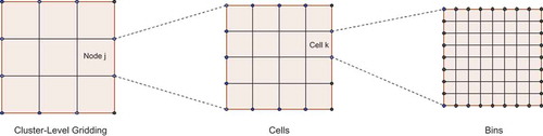
Bin Phase. After each node had received its entire allocation of points from the master, it then (and only then) proceeded to further partition the points into cells, and, within each cell, bins. This partitioning was accomplished by the primary thread on each node.

The physical regions assigned to each node, together with the cells assigned to each (worker) thread and the bins that made up the cells, constituted a three-tier hierarchical gridding of the entire physical region (Figure 2). This hierarchical grid was represented in memory as is (i.e., not using any ancillary data structure such as a quad-tree). In other words, memory was allocated for every bin in every cell on every node. On each node, the primary process (the process responsible for the socket connection to the master node, or the master process itself) subdivided its assigned partition into cells, where the number of cells was determined by the multiprocessing/multithreading capabilities of the individual machine. In the experiments, a homogeneous cluster in which every machine possessed the same number of (virtual) CPU cores (32), and ran the same number of threads, was used.

Each cell within the partition assigned to a node was further subdivided into bins. Since a point’s x- and y-coordinates were known to the machine/thread to which it had been assigned, assignment to the correct bin was only a matter of array-lookup. The bin table thus served as a large, two-dimensional hash-table in which the hash value was, straightforwardly, the (x,y)-physical location of a point. With sufficient memory at each node, cells could be subdivided such that the expected number of points destined for a single bin was approximately 1–2. The primary process on each node was responsible for placing each point assigned to that node into the bin table.

Filter Phase. After the primary process on each node had input and distributed every point in the physical region to be processed, and each node had constructed its local bin table data structure, a decimation (filtering) procedure was applied to reduce the total number of data points in the system. Specifically, points were filtered according to whether they might have constituted a significant feature in the local landscape; this analysis was performed by computing the local z-mean and z-variance (Section 2.1.1) and determining whether or not the local variance was above a predetermined threshold. If it was not, all points in the bin were removed (the bin was decimated).

Triangulate Phase. Within a cell, a single thread (the thread responsible for that cell) triangulated the reduced point cloud using a DT algorithm, which, in the implementation, combined features of both Watson’s and Lawson’s algorithms (Lawson 1977; Watson 1981). Initially, a bounding rectangle was trivially triangulated; points were then inserted into the existing triangulation one by one.

Figure 3. Location of the triangle containing the point under consideration.

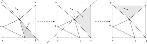
In Lawson’s approach, when a point (e.g., point H in Figure 3) is inserted, the triangle in which it currently lies must first be located. To accomplish this task, the most recently created triangle is tested for containment of the point. If the point is not contained in the triangle, then it will lie to the external side of some edge. For instance, point H is not contained in triangle BFE and lies to the outside of edge BF (Figure 3). This prompts the algorithm to next consider the triangle adjacent to BFE across edge BF. This sequence of steps is repeated until, in Figure 3, triangle DFC is found to contain the new point H.

After the addition of each point, the necessary ‘edge swaps’ were performed according to Lawson’s swapping algorithm (Lawson 1977). The performance of Watson’s algorithm (Watson 1981) is dependent on the order of insertion; since each thread possessed a hash-map structure for the data points, it was possible for the points to be triangulated in an order that resulted in fewer swappings and hence ‘good’ running-time behaviour. The C implementation used was derived from Sloan’s Fortran 77 implementation (Sloan 1987).

Once each cell (at each node) had been reduced and triangulated, the master thread on each server performed a ‘stitching-together’ of the triangulations of each cell by adding a certain number of artificial data points along cell boundaries and interpolating at each. The cell boundaries were one dimension smaller than the point cloud, and consequently, the addition of artificial boundary points did not change the data set size substantially. Thus, the final triangulation was only a true DT within each cell of each partition associated with each node.

Merge Phase. After the DTs of all cells had been stitched together by the primary thread on each node (into a triangulation, which was almost Delaunay, of that node’s entire partition), the master thread on each node transmitted its data output back to the master node, using buffering to provide maximal throughput. The master node streamed the triangulated regions to disk immediately.

Validation. Validation of the output TIN was done by computing the RMSE in the z-direction between 10,000 randomly chosen input points per node and the interpolated z-value at the same (x,y)-coordinates in the TIN model. For instance, if a data point was not removed during reduction, and remained as a vertex during triangulation, then the z-difference at that point would be zero for the purposes of validation (were that point to be chosen among the 10,000 validation points). Otherwise, for an input point chosen for validation but which was removed during reduction, the TIN triangle containing its (x,y)-coordinates was located and its z-value interpolated as the value such that (x,y,z) lay in the plane of the TIN model.

4. Experiments

4.1. Overview

The primary test data set consisted of a 400-tile (20-by-20) region making up most of Johnson County, Iowa, USA – specifically, a UTM rectangle in Zone 15 with minimum coordinates (596,000, 4,596,000) and maximum coordinates (636,000, 4,636,000), for a total area of 1600 km². This data set comprised 3.64 billion points, with a point density of approximately 2.275 points per square meter. In the experiments, all input files were formatted in ASPRS LAS File Format, version 1.0 (ASPRS 2003). In LAS v1.0 format, this data set was approximately 95 GB. As a second data set, for the scalability experiments, a subset of Johnson County consisting of a 7-tile-by-7-tile region (11.7 GB) was used.

Two sequences of experiments were performed: the first using the variance-filtering reduction and the second using a uniformly random reduction (in which points were selected at random for removal to create the more sparse point cloud for triangulation). In the two sequences of runs, relevant parameters (the variance threshold for filtering during variance-filtering runs and the probability of removal during random-filtering runs) were chosen so as to have pairs of runs, one using each reduction technique, with roughly equal point-reduction fractions. The purpose of these choices was to be able to make meaningful RMSE comparisons (between runs having nearly identical reduction fractions).

4.2. Results

4.2.1. Reduction quality

The first series of experimental results addressed the question of filtering quality. After-triangulation RMSE of two different filtering methods – random filtering (each point is removed or kept with a certain probability, independent of others) and the new variance-threshold-based filtering scheme – were compared. Because of the binning approach to storing the point-set in memory, both of these methods were linear-time operations on the point-set; thus, while the variance-threshold filtering technique required some additional time, this difference was a very small percentage of the overall run-time and is scalable.

Figure 4. Relationship between RMSE and variance-threshold input parameter in the processing of Johnson County data set using a 9-node cluster.

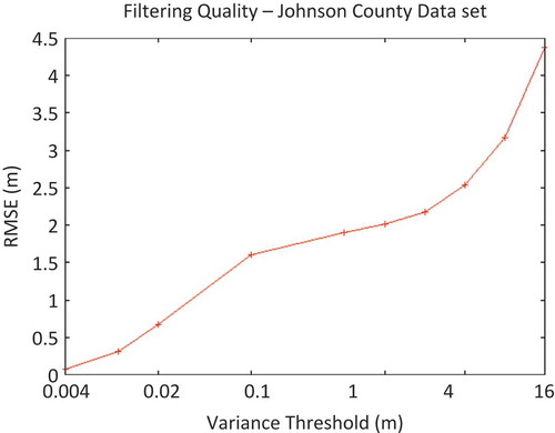
An interesting result of the experiments with the variance-threshold approach to data reduction was the roughly logarithmic relationship between the input variance threshold and the resultant triangulation RMSE (Figure 4). Without regard to performance variations of single-run experiments, there was a roughly linear relationship between the achieved TIN RMSE and the logarithm of the variance-filtering threshold.

Figure 5. Comparison of RMSE between filtering techniques, by reduction percentage (fraction of points decimated during filtering).

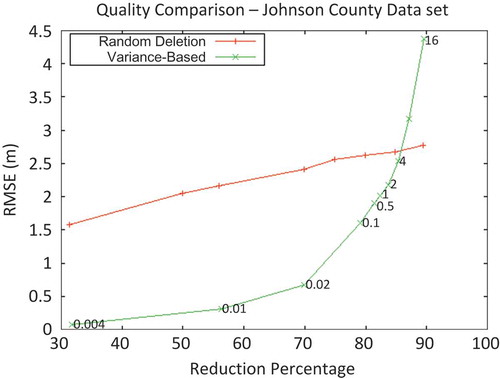
The results suggest that, when only moderate reduction of a data set is required, the variance-threshold-based approach to data reduction is superior to a filter that randomly deletes points to a desired percentage (Figure 5). Just as importantly, while the variance-based approach required an additional amount of time (compared to random deletion), this increase was insignificant in the context of total processing time. When high reduction of the input data set was pursued, however, the new approach performed no better than, or worse than, the random-filter control.

4.2.2. Scalability

The scalability of the written software was explored next. Using a 12.5-GB data set, the time required to process the data set with 1, 3, 6, and 9 nodes, and for several different reduction percentages, was measured. Since network communication was dependent on output data size, the filtering percentage played a role in determining the scalability.

Figure 6. Time per phase vs. cluster size for processing of Iowa City/Coralville data set with a variance threshold of 0.004 m.

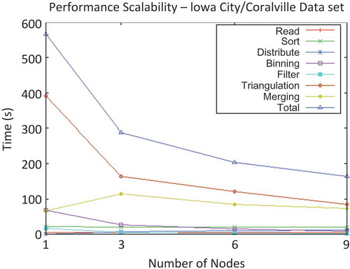
The task-stratified run-times of a single run instance are presented in Figure 6, as they illustrate an important point about the requirement that the data set be input and output on a single node at the beginning and end of the distributed processing. The merge phase run-time represents the time required for the master node to receive the triangulation output from each other node in the cluster, and write this output to disk. In a single-node ‘cluster’, there is no network communication, and so the ‘merge’ time is composed only of the time required to write to disk. Thus, an increase in the merge-phase time between the runs on the 1-node and 3-node clusters can be observed. This increase was due to the time required to transmit the triangulation output over the network (in the 3-node cluster). As the number of nodes increased, the time was amortized by the smaller loads on each server and decreased somewhat. However, it would never decay below the time necessary for a single node to write the entire output to disk, unless the requirement that the output reside on a single machine was obviated, say, by a distributed file system.

Figure 7. Total processing time vs. cluster size of Iowa City/Coralville data set for multiple threshold variances.

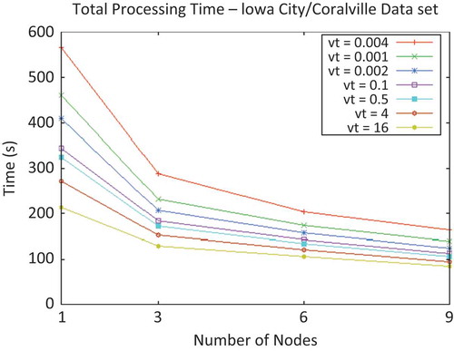
The total processing times on different-sized clusters, for a variety of input variance-threshold values, are depicted in Figure 7. A considerable reduction in running time is achieved, but linear speed-up is not observed due to the influence of sequential ‘critical sections’, such as reading and writing the input and output.

4.2.3. Processing time for large data sets

One of the purposes of this work was to show the practicality of processing (reducing and triangulating) large LiDAR data sets (the Johnson County data set was 95 GB in LAS format). As examples of the results, the following two experiments should be highlighted: (1) using a 9-node cluster, the software removed 32% of the points and triangulated the remaining Johnson County data set in 37 minutes, with an RMSE of 0.069 m; (2) using the same 9-node cluster, the software removed 81% of the points and triangulated the remaining Johnson County data set in 14 minutes, with an RMSE of 1.9 m. These results demonstrated the practicality of processing a large, unprocessed LiDAR data set on a small cluster when efficient software is used.

Figure 8. Time per phase vs. variance threshold for Johnson County data set.

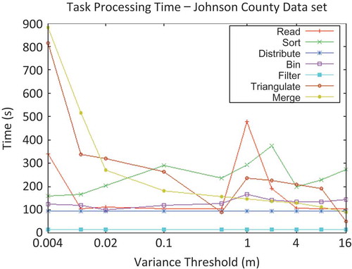
Any statistical properties are specifically disclaimed; since each parameterized run was performed only once, results are reported as single data points. In particular, in Figure 8, unexplained variability in identical tasks is apparent. (This explains the phenomena seen in Figure 9.) There is no algorithmic reason why the read, sort, or bin times should vary between runs; these steps occurred before any influence from the experimental parameter (the variance threshold) could have occurred. In contrast, the distribute phase is another step that should not (and did not) vary between runs; indeed, the network performance in the cluster was remarkably consistent.

Figure 9. Total processing time vs. variance threshold for Johnson County data set.

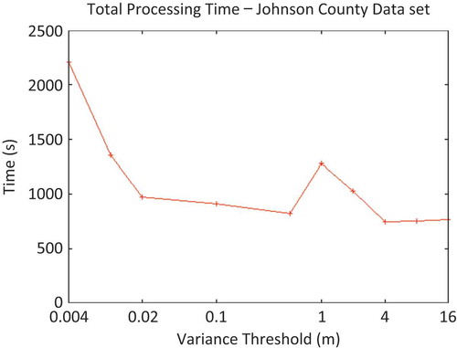
It should also be emphasized that significant portions of the experimental run-times observed were determined to be due to sequential aspects of the experimental set-up, which were nondistributable – e.g., for the purposes of comparison, the input data set and output triangulation were maintained on a single node (the master node). In a significant way, this requirement could be considered unfair to the larger clusters – the performance advantages of many distributed systems arise not just from the number of processors, but also from the duplication of other hardware components, such as disks.

4.3. Discussion and challenges

Several technical challenges of cluster computing had to be solved to optimize the experiments, and these are worth mentioning here. In HPC, and especially in data-centric applications, data transfers over various media must be carefully managed to obtain optimal results. While the media bandwidths of modern cluster components are quite high (500 MB/s to 1 GB/s SSD sequential read bandwidths; 10 Gbps ≈ 1 GB/s for high-speed ethernet), it is usually necessary to use careful buffering procedures to realize these speeds. Indeed, while AWS resources possessing 10-Gbps high-speed ethernet connections were used, it was found necessary to use large memory buffers to obtain reasonable performance during network transfers. Appropriate network flow control made an enormous difference – during the initial software testing, the processing of ~100 GB of LiDAR data was estimated to require over 3 hours; this was later reduced to 15–20 minutes by (1) reading the entire data set into memory prior to any other steps; (2) performing a bucket sort in RAM prior to point distribution in the distribute phase; and (3) transferring data points only in appropriately sized groups (making use of the prior bucket sort). These technical optimizations allowed the achievement of an actual data throughput (out of the master node) during the distribute phase of 8.6 Gbps, which is roughly optimal. The merge phase (involving the transmission of the output triangulation from each node’s region to the master node) was similarly optimized, although it should be noted that since the master node was also responsible for streaming the received triangulation directly to disk, run-times were not nearly as consistent as during the distribute phase.

5. Conclusions

In this article, the efficacy and scalability of using a distributed approach on a high-memory cluster to process large LiDAR data sets were examined. The importance of this work is driven by the ongoing expansion of memory sizes in commercial servers. The results demonstrate that (1) a point decimation based on local variance – which, in certain regimes, performed substantially better than randomized decimation – could be implemented in a high-memory cluster such that the additional required run-time was insignificant and that (2) data reduction and near-Delaunay TIN creation could be accomplished for data sets of the hundred-gigabyte scale in reasonable time frames and using reasonable machine resources. In conclusion, in the realm of spatial data, it was possible to use these next-generation memories to achieve a favourable time-space trade-off for typical processing operations. As well, a distributed approach to spatial data processing was still scalable, but did not exhibit the same level of linear scalability previously seen for systems and data sets where it was not possible to load the entire data set and associated data structures into system RAM.

These conclusions should not be misinterpreted as implying that the motivations for distributed approaches have declined recently. Indeed, it should be emphasized that the lack of true linear scalability in the distributed approach studied is mostly a consequence of (1) the restriction of single-node experiments to data sets small enough to be processed in RAM and (2) the lack of linear scalability in disk accesses. In regard to point (2), the experiments somewhat favoured the single-machine approach in that input and output were (artificially) required to reside on a single machine. The software was not allowed to take advantage of a distributed filesystem and the parallelization of disk access that would provide. Therefore, it is predicted that specialized distributed file systems (e.g., the Hadoop Distributed File System) may be a fertile area of research for data-centric application domains such as GIS.

Funding

This research was conducted with support from Amazon Research Grant (AWS) and USGS-AmericaView projects.

References

- Anderson, E. S., J. A. Thompson, and R. E. Austin. 2005. “LIDAR Density and Linear Interpolator Effects on Elevation Estimates.” International Journal of Remote Sensing 26 (18): 3889–3900. doi:10.1080/01431160500181671.
- ASPRS. 2003. “ASPRS LIDAR Data Exchange Format Standard Version 1.0.” The American Society for Photogrammetry and Remote Sensing. Accessed April 30, 2014. http://www.asprs.org/a/society/committees/standards
- AWS. 2014. “Amazon Web Services, Inc.” Accessed April 30. http//aws.amazon.com/ec2/
- Barr, J. 2006. “Amazon EC2 Beta.” Amazon Web Services Blog. Accessed April 30, 2014. http://aws.typepad.com/aws/2006/08/amazon_ec2_beta.html
- De Berg, M., M. Van Kreveld, M. Overmars, and O. C. Schwarzkopf. 2000. Computational Geometry. Secaucus, NJ: Springer.
- Dwyer, R. A. 1987. “A Faster Divide-and-Conquer Algorithm for Constructing Delaunay Triangulations.” Algorithmica 2 (1–4): 137–151. doi:10.1007/BF01840356.
- Isenburg, M., Y. Liu, J. Shewchuk, and J. Snoeyink. 2006. “Streaming Computation of Delaunay Triangulations.” ACM Transactions on Graphics (TOG) 25: 1049–1056. doi:10.1145/1141911.1141992.
- Kohout, J., I. Kolingerová, and J. Žára. 2005. “Parallel Delaunay Triangulation in E2 and E3 for Computers with Shared Memory.” Parallel Computing 31 (5): 491–522. doi:10.1016/j.parco.2005.02.010.
- Krishnan, S., C. Baru, and C. Crosby. 2010. “Evaluation of Mapreduce for Gridding LIDAR Data.” In 2010 IEEE Second International Conference on Cloud Computing Technology and Science (CloudCom), 33–40. Indianapolis, IN: IEEE.
- Lawson, C. L. 1977. “Software for C1 Surface Interpolation.” In Mathematical Software III, edited by J. R. Rice, 161–194. Pasadena, CA: Jet Propulsion Laboratory, California Institute of Technology.
- Lo, S. H. 2012. “Parallel Delaunay Triangulation – Application to Two Dimensions.” Finite Elements in Analysis and Design 62: 37–48. doi:10.1016/j.finel.2012.07.003.
- Oryspayev, D., R. Sugumaran, J. DeGroote, and P. Gray. 2012. “LiDAR Data Reduction Using Vertex Decimation and Processing with GPGPU and Multicore CPU Technology.” Computers and Geosciences 43: 118–125. doi:10.1016/j.cageo.2011.09.013.
- Peucker, T. K., R. J. Fowler, J. J. Little, and D. M. Mark. 1978. “The Triangulated Irregular Network.” In Proceedings of the Digital Terrain Models Symposium, 516–532. St. Louis, MO: American Society of Photogrammetry.
- Sloan, S. W. 1987. “A Fast Algorithm for Constructing Delaunay Triangulations in the Plane.” Advances in Engineering Software (1978) 9 (1): 34–55. doi:10.1016/0141-1195(87)90043-X.
- Watson, D. F. 1981. “Computing the N-Dimensional Delaunay Tessellation with Application to Voronoi Polytopes.” The Computer Journal 24 (2): 167–172. doi:10.1093/comjnl/24.2.167.
- Wu, H., X. Guan, and J. Gong. 2011. “Parastream: A Parallel Streaming Delaunay Triangulation Algorithm for LiDAR Points on Multicore Architectures.” Computers and Geosciences 37 (9): 1355–1363. doi:10.1016/j.cageo.2011.01.008.
- Yang, C., and Q. Huang. 2013. Spatial Cloud Computing: A Practical Approach. Boca Raton, FL: CRC Press.