A fast image rectification method for video captured with UAV hovering over traffic intersections

Abstract

With the development of UAV (Unmanned Aerial Vehicle) technologies, video clips recording high-resolution ortho-images covering intersections can be captured with video cameras mounted on a UAV at a given time and location. From these clips, traffic flow information can be derived. However, since UAV is easy to be affected by external atmospheric conditions, images in video clips may be jitter or unstable, which poses a challenge to automatic information extraction. This paper aimed to present a fast image rectification method to rectify geometric information for continuous images in UAV video clips. The proposed method is a feature-based approach especially for video clips covering traffic intersections with multiple groups of zebra lines. It consists of the following three steps: (1) zebra lines detection, (2) feature points calculation and (3) perspective translation. This approach is implemented and applied to an intersection video clip, and results demonstrate that the proposed method is able to correctly rectify most images in the clip and the rectifying rate is about 12.5 images per second.

Keywords:

• UAV (Unmanned Aerial Vehicle)
• traffic intersection
• zebra lines
• image rectification
• perspective transformation

1. Introduction

GIS-T (geographic information system for transportation) is currently recognized as an effective way to relieve traffic congestion and improve traffic efficiency in modern cities. A fundamental part of GIS-T is complete, timely and accurate traffic data covering road networks, especially intersections. Most existing approaches to traffic data collection, such as CCTV, induction coil, microwave detectors, etc. (Leduc 2008), collect lane-based information with high installation and maintenance cost but limited coverage. With the development of UAV technologies, videos covering traffic intersections or road segments can be captured with UAV cameras at a given time and location. Digital video processing technologies can help to derive semantic information (i.e. vehicle speed, delay, route, etc.) for GIS-T study.

Over the past decade, some researches were conducted to explore UAV applications in GIS-T. Ahmad and Samad (2010) used UAV to capture digital aerial photographs and produce topographic map and orthophoto. Feng, Yundong, and Qiang (2009) presented a real-time road mapping system based on UAV platforms. Liu et al. (2014) proposed a multi-objective optimization model of planning UAV route for road segment surveillance. Heintz, Rudol, and Doherty (2007) employed colour and thermal images of urban traffic captured with UAV to construct and maintain qualitative object structures and to recognize the traffic behaviour of vehicles, and finally, to achieve high level situation awareness about urban traffic situation. UAV is independent of ground facilities and able to reach appointed observation points conveniently. Compared with traditional traffic data collection methods, the UAV-based method is more flexible and its results are more complete. Although traditional CCTV can also capture traffic video, it is always mounted on a ground-based fixed position, and thus the recorded video is inevitably slant and likely to be shaded by large vehicles. Image fusion based on multiple cameras may help to achieve a complete spatial coverage, but it is still a challenge to synchronize spatial and temporal information among cameras even if there are enough cameras. By this meaning, the UAV-based method might be an alternative to traffic data collection. Figure 1 displays one image from an intersection video clip taken by a camera-equipped UAV.

Figure 1. A UAV image over a traffic intersection.

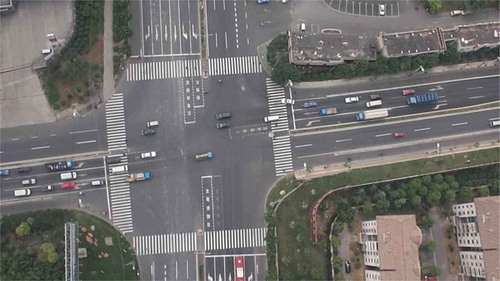
With respect to cost, technology, and portability, a UAV usually is of light weight. Due to varying atmospheric conditions, there is always a trade-off between weight and stability of UAV. The lighter a UAV is, the worse its stability. Accordingly, posture stability of UAV is easy to be damaged, and thus jittered or distorted images will be witnessed in UAV video clips. Rectifying these images is the first priority before traffic information extraction.

It is noted that there are usually a significant number of pixels representing moving objects (vehicles, pedestrians, bicycles, etc.) in a single image covering a traffic intersection, and these pixels or objects change location between successive images in a video clip. Existing image rectification methods are generally inadequate to rectify images that contain many spatially changing pixels (Reddy and Chatterji 1996; Zitová and Flusser 2003). In view of this, the purpose of this paper was to develop an appropriate method to rectify such images.

Traffic intersections, where traffic flows meet, are usually recognized as vital points in an urban road network. Traffic data around intersections are more significant and valuable than other traffic elements in GIS-T study. The proposed method is especially designed for intersections with multiple zebra lines. It uses zebra lines recognition, contour extraction, variance analysis, clustering, linear fitting and perspective transformation, etc., to implement a rapid image rectification.

The remainder of this paper is organized as follows. Section 2 reviews relevant aspects of image rectification methods. Section 3 proposes the principle and details of the proposed methodology. Section 4 implements and examines this method with a series of experiments. Finally, Section 5 summarizes the contributions of this paper and concludes with some ideas for future research in this area.

2. Review of image rectification methods

Image rectification methods can be divided into three categories: grey-information-based approaches, transform-domain-based approaches and feature-based approaches (Reddy and Chatterji 1996; Zitová and Flusser 2003).

Grey-information-based approaches usually have limited applications because they cannot correct nonlinear distortions (Zitová and Flusser 2003). In transform-domain-based approaches, Fourier transform, wavelet transform and Walsh transform methods are widely employed. For scaled, rotated and translated images, Reddy and Chatterji (1996) and Chen, Defrise, and Deconinck (1994) have developed a classical rectification algorithm based on Fourier transform method. Feature-based approaches extract multi-pairs of corresponding feature points between images and then use a transformation method to implement image rectification. Among them, Scale Invariant Feature Transform (SIFT) is proposed by Lowe (2004). SIFT method can robustly identify feature objects even with clutter or partial occlusion, because, to uniform scaling and orientation, its feature descriptor is identical, while, to affine distortion and illumination changes, the descriptor is partially invariant (Lowe 1999). However, the construction of the feature descriptor is complicated and the mechanism of choosing descriptors varies with different application scenarios (Lowe 2004). Based on SIFT, some alternative methods have been proposed, such as principle component analysis-SIFT (Ke and Sukthankar 2004), colour SIFT (CSIFT) (Abdel-Hakim and Farag 2006), Speeded-Up Robust Features (SURF) (Bay, Tuytelaars, and Van Gool 2006) and Affine-SIFT (ASIFT) (Morel and Yu 2009).

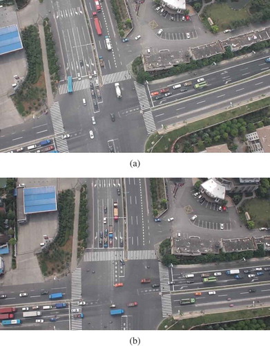
Because most of existing approaches implicitly share the same hypothesis that pixels or objects are always static in all images or the number of changing pixels is limited, there is still a requirement to develop rectification method for intersection images. Figure 2 demonstrates the phenomenon, where two images taken at different time instants from one video clip record traffic situation of the same intersection. Solid boxes in Figure 2a highlight vehicles passing through the intersection. These boxes are pasted to corresponding position in Figure 2b, and it is noted that pixels in every box have changed.

Figure 2. Significant number of pixels change from image (a) to image (b) which are from the same video clip.

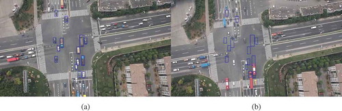
To tackle this problem, we develop a feature-based method, enlightened by RANSAC (RANdom SAmple Consensus) proposed by Fischler and Bolles (1981). RANSAC is an iterative method to estimate parameters of a mathematical model from a set of observed data including outliers. It is often applied in computer vision, such as simultaneously solving correspondence problems and estimate the fundamental matrix related to a pair of stereo images. In the light of this idea, the proposed method chooses zebra lines as features of each image, and feature points figured out from zebra lines are used in rectification. The principle and details of the method are given in the following section.

3. Methodology

3.1. Principles

In general, zebra lines have regular shape, colour and combination. As shown in Figure 1, there are four groups of zebra lines. For each group, the spacing between two zebra lines and the size of each zebra line are mostly identical. These geometric features of zebra lines in intersection are used to figure out feature points for the proposed image rectification approach. Figure 3 gives an overview of the approach, where diamond boxes and rectangle boxes represent data and procedures respectively, and directed arrows represent data flows and processing orders. It includes three steps: (1) zebra lines detecting, (2) feature points calculating and (3) perspective translation. In step 1, contour detecting algorithm (Suzuki and Abe 1985) is applied to each image to obtain contour sequence of zebra lines. Detected zebra lines are grouped based on their spatial relationship. In step 2, central points of zebra lines in each group are linked to construct reference lines and their cross points are employed as feature points of this image. In step 3, based on multiple pairs of feature points, perspective transformation method proposed by Mezirow (1978) is used to rectify images with respect to a reference image.

Figure 3. Overview of the proposed image rectification approach.

3.2. Detecting zebra lines

We apply a specific contour detecting method proposed by Suzuki and Abe (1985) to detect contours of zebra lines. The input of Suzuki method is a binary image, and it outputs contour sequences by means of traversing eight neighbouring pixels of all pixels of the binary image. One neighbouring pixel having a colour different from the central pixel is a boundary pixel, and, otherwise, it is an interior point. A contour is made up of a sequence of boundary pixels. Through setting appropriate binary and colour threshold, it is possible to detect contours of zebra lines. However, the accuracy of Suzuki method is influenced by image quality. For images from UAV video, weather conditions (sunny or cloudy) and recording sessions (morning, afternoon or evening) affect their brightness and resolution. Furthermore, UAV camera’s recording height is inversely proportional to the video clarity. Blurred edges and distorted colour are unavoidable in images. These issues increase the difficulty of image processing and contour extraction. As a result, the detected contours may include not only zebra lines but also other spots.

In response to these issues, three parameters of a contour, namely aspect ratio, area and colour, are defined to furthermore distinguish contours representing zebra lines from other spots. Since zebra lines usually have regular shape, size and colour, their corresponding contours should have similar aspect ratio, area and colour as well. Among these three parameters, aspect ratio, as a relative value, is generally a constant for zebra line contour in different images, and thus it is judged in advance. Area and colour of contour may vary with image due to different shooting position and brightness. Especially, the colour parameter is used to determine the value of binary threshold for converting a colour or grey image into a binary image, which is the input of Suzuki method. We proposed a method, as given in Algorithm 1, to implement the procedure of determining parameters and detecting contours for each image. The input is a grey image with n, such as 256, greyscales. The colour parameter is orderly assigned to a value from 1 to n, which, as a threshold, is used to convert the input image into a binary image. Then, with Suzuki method, a set of contours is obtained. Aspect ratios of these contours are compared with a predefined range, namely [minScale, maxScale], to remove outliers. minScale and maxScale can be determined by specific provision of local traffic laws or regulations, or obtained through field tests. The areas of the rest contours are calculated and sorted. A variance-based approach is then used to determine the area range of contours most likely representing zebra lines. Its principle is to sequentially remove the minimum area or the maximum area until the change of the remaining areas’ variance converges to a minimum value, and the range of the finally left areas is regarded as the area parameter of this image with current colour parameter. Contours are further filtered with the area parameter. After finishing the loop on all greyscales, we may obtain the optimal colour parameter, namely optColor, and the corresponding area parameters, namely [minArea, maxArea], with which, the maximum number of resulting contours can be obtained and these contours are return as the output of this algorithm.

Table

Algorithm 1: Determining parameters and detecting contours
Input: A grey image Output: A set of contours
Loop colour parameter∈[1, n]   Convert the input image into a binary image with colour parameter;   Use Suzuki method to obtain a set of contours;   Filter contours with aspect ratio, i.e., minScale and maxScale;   A variance-based approach is applied to calculate area parameters;   Filter contours with area parameters, i.e., minArea and maxArea;   Record the remaining contours;  End Loop  Find the set of contours with the largest number of contours;  Return this set as a result.

The output from Algorithm 1 may still include contours representing a few spots other than zebra lines. In the next step, most of them can be identified and removed.

3.3. Calculating feature points

For perspective transformation, at least four pairs of feature points are needed. Our approach is to group zebra lines, create axis of each zebra line group, and let the crossing points of axes be feature points.

Let D denote the spacing between two parallel zebra lines covering the same road segment. Its value can be determined in advance. The real distance between central points of contours can be calculated from Algorithm 1. Through comparing these distances with D, it is able to group contours representing zebra lines crossing different road segments. Let S_k denotes a set of central points of the kth contour group. Due to the existing of noise spots, the central points of contours may not be always identical to those of zebra lines. Therefore, if the number of central points in a set is less than a predefined threshold, the set are regarded as a false one and rejected.

In principle, the central points of zebra lines belonging to the same group are on the same straight line, i.e. axis of the group. The least squares method (Charnes, Frome, and Yu 1976) is employed to build the axis. Let p_i = (x_i, y_i) denote one central point in S_k, where x_i and y_i are coordinates of p_i. Let denote the average of x_i, denote the average of y_i. The linear equation of the axis is a_kx − y + b_k = 0, where a_k and b_k are calculated with Equations (1) and (2).

(1)

(2)

Because of the coverage of passing vehicles, zebra lines covering the same road segment may be broken in images and classified into several groups, and thus, some axes obtained above should be merged. If two axes are nearly parallel and close to each other, they are merged as a single axis and their corresponding central point sets are combined as well. To further removed false axes, for each central point set S_k, we calculate S_k’s linear correlation coefficient, namely r_k, between variables x and y. If , where R is a predefined threshold less than one, the set and its corresponding axis are removed.

With the resulting axes, it is able to find crossing points among them for each image. If the number of points is more than four, these points can be employed as feature points of this image to feed perspective transformation.

3.4. Perspective transformation

First, a reference image needs to be determined. It can be the first image in a video clip with enough number of feature points. Then, other images are converted into new images with a spatial framework identical to that of the reference image through perspective transformation (Mezirow 1978), as shown in Equations (3)–(5), where x and y are coordinates of a pixel in a raw image, x′ and y′ coordinates of a converted in its rectified image, and a, b, c, d, e, f, g and h is the conversion factor.

(3)

(4)

(5)

For any raw image with more than four feature points, its eight conversion factors can be obtained through solving a equation group given in Equation (6), where (x₁, y₁), (x₂, y₂), (x₃, y₃) and (x₄, y₄) are coordinates of four feature points in the raw image, and (x₁′, y₁′), (x₂′, y₂′), (x₃′, y₃′) and (x₄′, y₄′) are coordinates of four feature points in the reference image.

(6)

4. Experiments

The proposed approach is applied to an intersection video clip. The hovering height of UAV is about 120 meters. The length of video clip is 243 seconds with a frame rate of 30 frames per second. Each frame is an image with the same resolution of 1280 × 720 pixels. Video clip recorded in the morning with high visibility and breeze. The approach is implemented with C++ of Microsoft Visual Studio 2008, and experiments are conducted on a computer equipped with Intel i5 3.2 GHz CPU, 2 GB RAM and Windows 7 64-bit operating system.

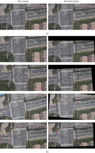
Figure 4 illustrates some snapshots of image rectification. Figure 4a gives the reference image. Figure 4b gives some other images. Raw images are listed on the left side and rectified images on the right side. In these images, solid line boxes and dashed boxes indicate the range of zebra lines before rectification and after rectification, respectively. It is noted that both boxes in the reference image keep the same position, while changing in other images. Two short video clips are also attached to this paper to demonstrate the deference before and after rectification. The remainder of this section presents the process of zebra lines detection, feature points calculating and perspective transformation.

Figure 4. Examples of image rectification for rectifiable images (b) according to a reference image (a).

4.1. Zebra lines detection

First, Algorithm 1 is used to detect zebra lines. In this experiment, minScale = 8 and maxScale = 14. Other parameters, i.e. optColor, minArea and maxArea, can be calculated with Algorithm 1. The greyscale is from 1 to 256. Results are illustrated in Figure 5, giving the value of optimal colour parameter (Figure 5a) and minArea and maxArea (Figure 5b) of each image. It validates the necessity of Algorithm 1 about the trend of these parameters, and shows that filter parameters of every image are different and unsteady which due to the content, colour and shape of images has some changes caused by lighting and atmosphere change. It can be seen that constant filter parameters cannot be used to detect contours of zebra lines and dynamic parameters must be used to meet the requirement of contour detection.

Figure 5. Value of optimal colour parameter (a) and minArea and maxArea (b) of each image.

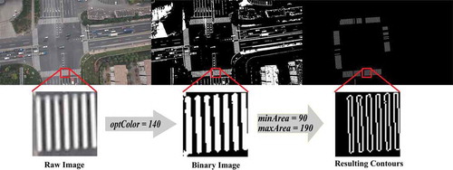
Figure 6 is the process of contour detection in the reference image, where optColor = 140, minArea = 90 and maxArea = 190. The number of detected contours is 119.

Figure 6. The process of contour detection in the reference image.

4.2. Calculating feature points

In this experiment, D is taken , and , respectively, where denotes the average height of all contours in one image. The least number of central points is assigned 4. Then, detected contours can be grouped according to central point clustering.

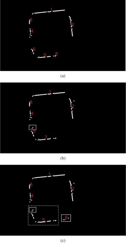
Figure 7 illustrates the result of central point clustering when D equals different values. The change from Figures 7a to 7c shows the influence of D on the result. The smaller the value of D is, the more the number of categories there are. In Figure 7b, central points are aggregated into seven categories, and class 6 is removed because its point number is less than 4. In Figure 7c, a relative larger D leads to those central points at lower left corner belonging to different road segments are classified into one class. We select as the value of D to group contours.

Figure 7. Results of central point clustering when D = (a), (b) and (c).

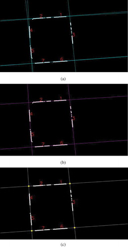
Figure 8 illustrates the process of calculating feature point. Figure 8a shows the result of drawing fitted axis for each group of central points. There are totally seven lines. Figure 8b gives the result of axis merging, where angle threshold is set to 45°. After merging, 4 lines are remained. Figure 8c highlights the 4 crossing points of these 4 lines. For the reference image, coordinates of the 4 feature points are (286.25, 186.87), (698.26, 160.97), (745.67, 601.90) and (316.53, 632.43), respectively.

Figure 8. The process of calculating feature point from building axes (a), merging axes (b) and obtaining crossing points of axes (c).

4.3. Perspective transformation

Like the reference image, feature points of images can be calculated in the same way. If an image has four feature points as shown in Figure 8c, then it is a rectifiable image, and perspective transformation can be applied. The statistical results of image rectification are given in Table 1. The number of rectifiable images is 6025, 82.57% of the total. Images fail to be rectified are divided into the following three cases, missing zebra lines (1146, 15.71%), fail to detecting zebra lines (86, 1.17%) and wrongly detecting images (40, 0.55%). Some failure cases are demonstrated in Figure 9, where a significant part of zebra lines are missed due to heavy jittering.

Table 1. The statistical results of images rectification.

Video frame type	Feature points number	Quantity	Proportion (%)
Rectified images	4	6025	82.57
Other images	≤4	1272	17.43
Missing zebra lines	<4	1146	15.71
Fail to detecting zebra lines	<4	86	1.17
Wrongly detecting	4	40	0.55
Total		7297	100

Figure 9. Two examples of images fail to be rectified.

4.4. Performance analysis

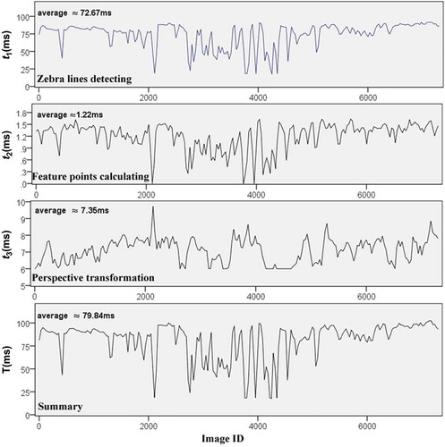
Figure 10 gives the computational time spent for rectifying each image, where the horizontal axis is image identification, and the vertical axis computational time of whole process and single stages including zebra lines detection (t₁), feature points calculating (t₂) and perspective transformation (t₃). Zebra lines detection is always the most time-consuming stage. t₁ and t₂ have similar curves because both stages are highly correlated to each other.

Figure 10. Computational time of image rectification.

To examine the accuracy of the proposed method, we randomly select some sample points commonly existing in the reference image and rectified images and compare their spatial error. For example, if one sample point in a rectified image is located at (x₁, y₁), and in the reference image, its coordinates are (x₀, y₀), then the error of this point equals . Figure 11 gives a frequency map representing error distribution, where the horizontal axis is error in pixel, and the vertical axis is the number of points. The map shows that most errors are less than two pixels. A possible reason is the conversion between integer and real during rectification. Images are composed of pixels representing with integer, while perspective transformation is based on real. Therefore, accuracy has to be compromised when converting from real to integer.

Figure 11. Error analysis.

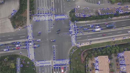
To evaluate the effectiveness of the developed method, comparisons between our method and SURF method (Bay, Tuytelaars, and Van Gool 2006) are performed here. SURF is a robust local feature detector and is partly inspired by the SIFT descriptor, but much faster than SIFT. SURF is also a feature-point-based approach. It usually can detect a large number of feature points, from which RANSAC is used to exclude mismatching feature point pairs and build optimal transformation matrix.

Table 2 gives the result of comparison between the proposed method and SURF+RANSAC method. An image from experimental video clip is selected randomly to be rectified. The rectifying errors of two methods are similar. With SURF + RANSAC method, much more feature point pairs are obtained with larger computational time than our method. Figure 12 shows these feature points, i.e. points, detected by SURF method. This explains that why SURF + RANSAC method takes more time than the proposed methods. Computational time is critical when dealing with a large number of pictures, if similar results can be guaranteed. By this means, the proposed method outperforms the SURF + RANSAC method.

Table 2. Results of comparison.

Method	The number of feature point pairs	Computational time (millisecond)				Rectifying errors
		Detecting feature points	Matching feature points	Calculating optimal transformation matrix	Rectifying image
The proposed method	4	79	1	1	7	less than 2 pixels
SURF + RANSAC	1211	288	119	54	6	less than 2 pixels

Figure 12. Feature points detected by SURF method.

5. Conclusion

Using UAV video clips at traffic intersection to quickly derive traffic flow information and to evaluate the quality of traffic service is a novel method of traffic data collection. A fundamental work is to overcome the problem of video jitter caused by UAV shaking and weather conditions. In view of this, the paper proposed a rapid feature-based image rectification method. It is especially applicable to video clips covering traffic intersections with multiple groups of zebra lines. It consists of the following three steps: (1) zebra lines detection, (2) feature points calculation and (3) perspective translation. This approach is implemented and applied to an intersection video clip, and results demonstrate that the proposed method is able to correctly rectify most images in the clip. Its spatial errors can be mostly limited within 2 pixels. Its rectifying rate is about 12.5 images per second. Considering the actual requirement of vehicles detection, real-time rectification can be achieved by reducing sampling rate.

Future efforts are focused on the improvement of performance and accuracy, and more general methods applicable to other scenarios, such as an intersection with only two groups of or without zebra lines, needs to be developed.

References

- Abdel-Hakim, A. E., and A. A. Farag. 2006. “CSIFT: A SIFT Descriptor with Color Invariant Characteristics.” Paper presented at the IEEE Computer Society Conference on Computer Vision and Pattern Recognition 2: 1978–1983.
- Ahmad, A., and A. M. Samad. 2010. “Aerial Mapping Using High Resolution Digital Camera and Unmanned Aerial Vehicle for Geographical Information System.” Paper presented at the 6th International Colloquium on Signal Processing and Its Applications (CSPA), 1–6. IEEE. doi:10.1109/CSPA.2010.5545303.
- Bay, H., T. Tuytelaars, and L. Van Gool. 2006. “SURF: Speeded up Robust Features.” In Computer Vision–ECCV 2006, edited by A. Leonardis, H. Bischof, and A. Pinz, 404–417. Berlin: Springer.
- Charnes, A., E. L. Frome, and P. L. Yu. 1976. “The Equivalence of Generalized Least Squares and Maximum Likelihood Estimates in the Exponential Family.” Journal of the American Statistical Association 71 (353): 169–171. doi:10.1080/01621459.1976.10481508.
- Chen, Q.-S., M. Defrise, and F. Deconinck. 1994. “Symmetric Phase-Only Matched Filtering of Fourier-Mellin Transforms for Image Registration and Recognition.” IEEE Transactions on Pattern Analysis and Machine Intelligence 16 (12): 1156–1168. doi:10.1109/34.387491.
- Feng, W., W. Yundong, and Z. Qiang. 2009. “UAV Borne Real-Time Road Mapping System.” Paper presented at the Joint Urban Remote Sensing Event, 1–7. IEEE. doi:10.1109/URS.2009.5137476.
- Fischler, M. A., and R. C. Bolles. 1981. “Random Sample Consensus: A Paradigm for Model Fitting with Applications to Image Analysis and Automated Cartography.” Communications of the ACM 24 (6): 381–395. doi:10.1145/358669.358692.
- Heintz, F., P. Rudol, and P. Doherty. 2007. “From Images to Traffic Behavior-A UAV Tracking and Monitoring Application.” Paper presented at the 10th International Conference on Information Fusion, 1–8. IEEE. doi:10.1109/ICIF.2007.4408103.
- Ke, Y., and R. Sukthankar. 2004. “PCA-SIFT: A More Distinctive Representation for Local Image Descriptors.” Paper presented at the Proceedings of the IEEE Computer Society Conference on Computer Vision and Pattern Recognition, CVPR 2004, Vol. 2, II-506-II-513. IEEE. doi:10.1109/CVPR.2004.1315206.
- Leduc, G. 2008. “Road Traffic Data: Collection Methods and Applications.” Working Papers on Energy, Transport and Climate Change 1: 55.
- Liu, X.-F., Z.-W. Guan, Y.-Q. Song, and D.-S. Chen. 2014. “An Optimization Model of UAV Route Planning for Road Segment Surveillance.” Journal of Central South University 21: 2501–2510. doi:10.1007/s11771-014-2205-z.
- Lowe, D. G. 1999. “Object Recognition from Local Scale-Invariant Features.” Paper presented at the Proceedings of the Seventh IEEE International Conference on Computer Vision, Vol. 2, 1150–1157. IEEE. doi:10.1109/ICCV.1999.790410.
- Lowe, D. G. 2004. “Distinctive Image Features from Scale-Invariant Keypoints.” International Journal of Computer Vision 60 (2): 91–110. doi:10.1023/B:VISI.0000029664.99615.94.
- Mezirow, J. 1978. “Perspective Transformation.” Adult Education Quarterly 28 (2): 100–110. doi:10.1177/074171367802800202.
- Morel, J.-M., and G. Yu. 2009. “ASIFT: A New Framework for Fully Affine Invariant Image Comparison.” SIAM Journal on Imaging Sciences 2 (2): 438–469. doi:10.1137/080732730.
- Reddy, B. S., and B. N. Chatterji. 1996. “An FFT-Based Technique for Translation, Rotation, and Scale-Invariant Image Registration.” IEEE Transactions on Image Processing 5 (8): 1266–1271. doi:10.1109/83.506761.
- Suzuki, S., and K. Abe. 1985. “Topological Structural Analysis of Digitized Binary Images by Border Following.” Computer Vision, Graphics, and Image Processing 30 (1): 32–46. doi:10.1016/0734-189X(85)90016-7.
- Zitová, B., and J. Flusser. 2003. “Image Registration Methods: A Survey.” Image and Vision Computing 21 (11): 977–1000. doi:10.1016/S0262-8856(03)00137-9.