Human mobility patterns in different communities: a mobile phone data-based social network approach

Abstract

Detecting intensely connected sub-networks, or communities, from social networks has attracted much attention in social network studies. The widespread use of location-awareness devices provides a novel data source for constructing spatially embedded networks and uncovering spatial features of different population groups. Using an empirical mobile phone data-set, this paper attempts to explore the spatial distributions and human mobility patterns, as well as the interrelationship between them, at the community level. Three spatial patterns of communities are identified with the community detection algorithm and kernel density map method: single-centred distribution, dual-centred distribution and zonal distribution. We find different movement characteristics of these three community types by analysing angle distribution of trajectories and radius of gyration of users. Furthermore, we analyse spatial and temporal travel patterns for the users in dual-centred communities. The results indicate that people’s commuting travel brings about spatial interaction between urban district and suburbs, and verify our hypothesis that the distance decay effect along with social phenomena such as the home–work separation contributes to the formation of different community distributions.

Keywords:

• spatial pattern
• social community
• human mobility
• mobile phone data

1. Introduction

With the development of communication technology and the wide use of location-awareness devices, such as GPS-enabled devices and mobile phones, a great amount of geo-tagged data has been produced, making it possible to collect large-scale individual trajectories and interactions within social networks. Mobile phone data have unique characteristics to help us analyse human mobility and spatial interactions in both physical space and cyberspace. Caller connections usually correspond to everyday social relations. Although a mobile phone social network cannot completely represent a face-to-face network, it reflects people’s social relations better than online social networks such as Facebook, Twitter and Foursquare, in which people with hundreds of contacts may never physically meet. Furthermore, mobile phone communications are geo-located by mobile base towers nearby. This feature provides us opportunities to explore spatial structure of social network as well as people’s mobility.

The increasing availability of mobile phone data in recent years has triggered a range of studies: human mobility pattern (Brockmann, Hufnagel, and Geisel 2006; González, Hidalgo, and Barabási 2008; Song, Koren, et al. 2010; Song, Qu, et al. 2010), socio-economic factors and geography of social networks (Eagle, de Montjoye, and Bettencourt 2009; Krings et al. 2009; Eagle, Macy, and Claxton 2010; Onnela et al. 2011; Kang et al. 2012) and structures of social networks (Hidalgo and Rodriguez-Sickert 2008; Palla, Barabási, and Vicsek 2007). Recently, more studies have been carried out from a perspective of spatial social networks, which refer to social networks where nodes and edges are embedded in space. At the aggregate level, related studies applied mobile phone data to measure interaction between places for spatial regionalization and discovered that communities extracted from place-based networks often correspond well with administrative boundaries (Ratti et al. 2010; Gao et al. 2013). At the individual level, there exist a number of studies on relationship between mobility and social ties: Phithakkitnukoon, Smoreda, and Olivier (2012) found that a large portion of places visited are within several social circles centred at their nearest social ties’ locations. Eagle, Pentland, and Lazer (2009) found that friend dyads demonstrate distinctive temporal and spatial patterns in their physical proximity and calling patterns. However, few studies have inspected spatial pattern and human mobility pattern from a perspective of social community. A social community encourages people to engage in the exchange of information, and learn from each other. Social communities are not solely about aggregating information or resources, but about bringing people together to meet their social needs (Hagel 1999). Because people get social support mainly from community ties such as friends and relatives (Wellman and Wortley 1990), it is meaningful to explore spatial and mobility pattern at a social community level.

Given that population heterogeneity is an important factor in interpreting human mobility patterns (González, Hidalgo, and Barabási 2008), finding urban population groups using community detection provides an effective approach to take population heterogeneity into consideration. In this study, we attempt to investigate spatial pattern of urban population communities and compare mobility characteristics of different communities using mobile phone data. In achieving these goals, we adopt a community detection algorithm to study the patterns of individual communities and employed a kernel density estimation method to illustrate spatial distributions of extracted communities. Considering communities of different patterns, we explore the formation mechanism and mobility characteristics of members in different communities. Additionally, for communities with a dual-centred spatial distribution pattern, we analyse the spatiotemporal features of human trajectories and verified the supposition that distance decay effect along with particular social phenomena such as the home–work separation contributes to the formation of different community patterns. This research can improve our understanding to individual community patterns and spatial impacts on the formation of different community patterns.

2. Data description

2.1. Data-set

This study is conducted based on an anonymized data-set of nearly 1,000,000 mobile users in Harbin, a large city in northeastern China, over 1 month. Each entry in the data-set has a call detail record (CDR) containing the information of server number, opposite number, date, time, duration and the base tower through which the call is routed. When a call is made, the user’s location is approximated by the position of a nearby mobile base tower and recorded. The data-set covers 618 mobile base towers with geographical coordinates, which are highly clustered in urban areas and sparse in suburban areas (Figure 1). We use Thiessen polygons (termed ‘cell’) to approximate the coverage area of mobile base tower (Kang et al. 2012; González, Hidalgo, and Barabási 2008). The average cell area in the whole study area is 4.0 km², and the average distance between cells is 7.95 km. To ensure the accuracy of users’ mobility patterns, 537,718 mobile phone users whose locations were exposed at least ten times were selected from the data-set.

Figure 1. Spatial distribution of mobile base towers (dots) and associated Thiessen polygons. © [OpenStreetmap and contributors]. (The base map is obtained from OpenStreetmap, following the creative commons-share alike license. http://creativecommons.org/licenses/by-sa/2.0/)

2.2. Estimating home and workplace locations

Human trajectories show a high degree of temporal and spatial regularity. Each individual has a significant probability to return to a few frequented locations such as home and workplace (Song, Qu, et al. 2010). Based on this assumption, we estimate the home location as the cell tower location in which the user has the highest frequency of call activities during night-time hours (10 pm–6 am) (Phithakkitnukoon, Smoreda, and Olivier 2012). Similarly, the workplace is estimated as the most frequented cell tower location during work hours (9 am–12 am, 2 pm–5 pm). To ensure the accuracy, the estimation of home or workplace is adopted only when the highest frequency is greater than 40% and the calling times exceed 10. There exists an inherent limitation that the estimated location is defined as the centroid of the coverage area of a mobile base tower, not the same place with the exact home or workplace. However, it is currently the most reasonable way to estimate the location of home and workplace. Given that the distance between home and workplace of an individual represents his (or her) commute distance, we define home–work-separate people as individuals whose home and workplace locate in different cells in this paper.

2.3. Constructing mobile phone social network

Based on the reciprocal communications between users, we construct a weighted undirected network in which nodes are mobile phone users and edges are weighted by the total volume of phone-call interaction between users. We term this network as a mobile social network in which individuals connect with one another through their mobile phones. The resulting network is composed of 537,718 nodes connected by 1,251,645 undirected edges with an average degree <k> of 4.7. Lambiotte et al. (2008) analysed a mobile phone data-set over a period of 6 months and the resulting network has an average degree of 4.3, which is close to our finding.

In the research of complex network, degree of a node indicates the number of its connections with other nodes. A giant component is a giant connected subnet of a network used to quantify connectivity of the network (Erdős and Rényi 1960). The distribution of degree (Figure 2A) shows the characteristic of heavy tail, indicating that a relatively large fraction of people have high degrees. This is consistent with the findings in earlier research (Onnela et al. 2007).

Figure 2. Basic features of mobile social network. (A) Complementary cumulative distribution of degree; (B) Relationship of giant component’s size versus call frequency threshold. The giant component of the original network contains more than 96% of the nodes.

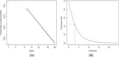
The network contains 7249 connected subnets and the largest one covers 96% of all nodes. To explore the stability of the network, we evaluate the impact of removing ties by measuring the relative size of giant component. Figure 2B illustrates how the percentage of nodes in giant component gets smaller along with the increase of the threshold. We find that the initial network has a rather good connectivity and the global connectivity becomes weaker as the threshold increases. The count of nodes reduces to half of its original size when the threshold reaches 3. The network collapses rapidly when weak ties are removed, consistent with the weak tie theory (Granovetter 1973).

3. Spatial distributions of urban population communities

3.1. Community detection

In complex network sciences, a community is defined as a group of densely connected nodes (Wellman 1999). In other words, communities are subsets of nodes within which vertex–vertex connections are dense, but between which connections are less dense (Girvan and Newman 2002). The identification of such groups is called community detection. Community detection provides us a new perspective for understanding the structure of mobile social network. As nodes in our mobile social network stand for individuals, communities detected from the mobile social network can be used to make an analysis at the social community level.

Newman and Girvan (2004) proposed the modularity measure to evaluate the quality of result from community detection. Modularity compares a specific partition to a null model with random connections. Higher value of modularity indicates a more robust community structure. Clauset, Newman, and Moore (2004) proposed the fast greedy algorithm which applies modularity as the criterion to construct communities. The division with the largest modularity is chosen as the result of community detection. We employ this method to extract ‘social communities’ because of its capacity to support large-scale networks. The result of community detection consists of 8495 communities and the modularity is 0.914, indicating a strong community structure. The number of communities containing 100+ individuals is 342 because many small isolated cliques including friend pairs or triples have connections only within the clique but no connection with other cliques. These small isolated cliques cannot reflect common features of communities. Therefore, we only choose 25 communities that contain more than 5000 individuals. People in these communities cover 40% of all users in the network.

3.2. Three types of individual spatial distributions

Based on the estimated home location of each individual, we could determine a spatial extent for each community. Hence, a community in this research possesses two implications: a sub network and a region, which may be disconnected, in physical space. In order to map a sub network to a region and weaken the impact of the uneven distribution of the cells, the study area is discretized into 0.5 × 0.5 km grids. Each individual is assigned to a grid randomly in its belonging cell area according to the estimated home location, which could make the visualization of spatial distribution more clear. For the extracted communities, we employ the kernel density estimation (KDE) method to find characteristics of individuals’ communities. Bandwidth (also called search radius) is the most important criterion in determining an appropriate result of density map. The choice of bandwidth will affect the spatial distributions of communities. To achieve an appropriate outcome of visualization, the bandwidth for this study is 1.5 km, which is three times of the grid size. Most maps present an appearance of single-centred pattern (Figure 3). We find that individuals among a community tend to be distributed in a spatial coherent region. Note that such a characteristic of spatially consecutive areas is found just by the total volume of phone-call interaction between users without considering the geographical adjacency constraint in the algorithm. This characteristic of our individual-based network is similar to the results of existing research on region-based networks (Ratti et al. 2010; Thiemann et al. 2010; Kang et al. 2013; Gao et al. 2013; De Montis, Caschili, and Chessa 2013). Recently, Liu et al. (2014) pointed out that the distance decay effect results in the spatial continuity of communities. Although Pfaff (2010) argued that mobile phones lead to the diminishing of physical distance constraints, we confirm that individuals are still more likely to form a social community with people nearby, which agrees with the first law of geography (Tobler 1970).

Figure 3. Spatial distributions of single-centred communities. Figure A, B and C show the small single-centred communities, while D, E and F show the large single-centred distributions.

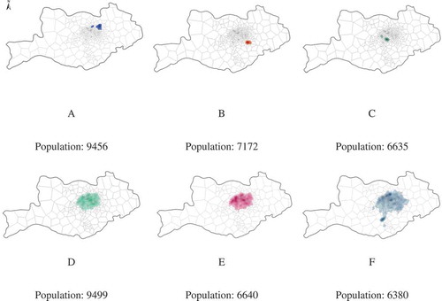
The differences among individuals’ behaviour characteristics lead to different community sizes and shapes. Some communities cover large regions (Figure 3D, E, F) while others cover comparatively smaller regions (Figure 3A, B, C). We term the former pattern ‘large single-centred pattern’ and the other ‘small single-centred pattern’. This research identifies 10 large single-centred communities and 5 small single-centred communities.

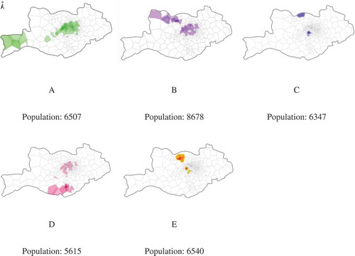
As shown in Figure 4, another type of community spatial distribution comes into our sight. These distributions exhibit a dual-centred pattern, indicating that some individuals cluster in a centre while the others cluster in a different place. The results of community detection contain five dual-centred communities. It is supposed that the characteristic of dual-centred distribution may be caused by the home–work separation (Schnore 1954). Today in many cities, residential and occupational locations are spatially divorced (Poston 1972). Daily journey to work has been a part of life for many people. Communities extracted from the individual network are usually composed of colleagues who contact each other frequently at work. Among them, some people live in a place near the work place while others usually live far away from the work place. The distributions of these two kinds of people lead to such spatial patterns of the communities.

Figure 4. Spatial distributions of dual-centred communities.

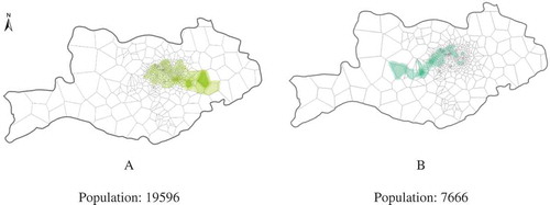
In addition to the two above mentioned patterns, Figure 5 illustrates two typical zonally distributed communities. Five of the twenty-five chosen communities possess a characteristic of ‘zonal pattern’. It can be regarded as the intermediate pattern between the single-centred one and the dual-centred one. People in each community are distributed in a band connecting a residential region and an occupational one. We suggest that the zonal area be a result of a spatial coherent area affected by social phenomena such as the home–work separation.

Figure 5. Spatial distributions of zonal communities.

3.3. Mobility characteristics of different community types

To compare the mobility patterns between these three types of communities, we investigate the distributions of two measures: direction and radius of gyration (ROG). The mobility direction of users accounts for the angle between the displacement and the horizontal line, while ROG measures a user’s activity territory. González, Hidalgo, and Barabási (2008) define the ROG as

where m represents the number of points in each user’s trajectory; and represent the ith position recorded for a user; and denote the centre of the trajectory. ROG is determined by the most frequent visited locations and less affected by rarely visited locations.

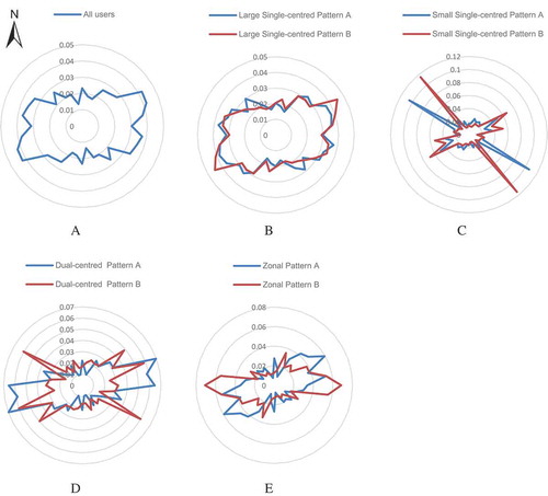
The angle is the direction of vectors composed by two successive trajectory points. Figure 6 is depicted by summarizing the frequency of the degree distribution with the bin size of 10 °. The angle distribution of all users displays in the direction of east and west (Figure 6A), which corresponds with the east–west direction of the study area. Also, it is natural that all these three pattern communities have an east–west main direction (Figure 6B, C and D). People would contact more frequently with others in their communities, leading to the similarity of outline between the community and the angle distribution. However, the angle distribution of small single-centred communities does not correspond with the outline of communities. The high probability of certain angle in small single-centred communities denotes that users who live close have a high moving direction preference. Large single-centred communities display the similar angle distribution to that of all users, meaning that users in large single-centred communities can reflect the angle characteristic of all users. The dual-centred community A has two centres which are located as the east–west direction. People would be inclined to move from one centre to another, leading to the east–west direction of angle distribution. The direction between two centres in dual-centred community B displays a high probability in the angle distribution. However, there exist other main directions of angle distribution, which means that the mobility pattern of users is not simply moving from one-centre to another. The movement within each centre would also affect the angle distribution such that the main direction of angle distribution in zonal communities corresponds with the main direction of zonal communities.

Figure 6. The angle distribution of different communities. For simplicity, we only choose two communities of each pattern to display their angle distributions. The community identifier in the legend of each pattern corresponds to Figures 3, 4 and 5.

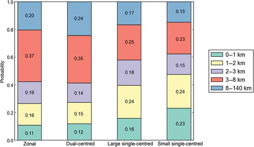
The proportion of users in dual-centred communities with ROG larger than 3 km is the highest, while that in small single-centred communities is the lowest (Figure 7), meaning that there are more people with long travel distances in dual-centred communities. This is reasonable if we assume that people usually travel within their communities (Phithakkitnukoon, Smoreda, and Olivier 2012). People who travel in a dual-centred community have naturally a longer distance than those who travel within a small single community. Some people in dual-centred communities move from one centre to another. This leads to an assumption again that people’s home and work place are separated in different centres. The long distance from home to work leads to the high probability of large ROG. We would verify this assumption in the following section.

Figure 7. ROG distribution of different community patterns. The order of the proportion of users with ROG smaller than 3 km is small single-centred, large single-centred, zonal and dual-centred. The majority (more than 60%) of users in small single-centred communities have ROG less than 3 km. The proportion of users in dual-centred communities is the largest to have ROG larger than 3 km. The ROG of more than 20% of users in dual-centred communities are larger than 8 km.

4. Trajectory analysis of dual-centred communities

Dual-centred pattern, as an anomaly spatial distribution pattern, contains a complex formation mechanism. Spatiotemporal analysis of human trajectories in dual-centred communities is valuable for understanding mobility pattern at community level and exploring spatial effects on the formation of communities. To verify the supposition that the home–work separation may contribute to the formation of dual-centred communities, we focus on analysis of home–work-separate persons’ trajectories.

4.1. Comparison of human trajectories in urban centres and suburban centres

With the inspection of spatial distributions of dual-centred communities, we can find that there exist one centre in the urban district and another centre in suburbs commonly for each community. Mobility patterns of individuals in different centres may be rather distinct.

As shown in Figure 8, we define ‘urban centre’ and ‘suburban centre’ as covered regions of two centres in the urban district and suburb, respectively. Using the set of trajectory points of home–work-separate people in urban centre, we yield trajectory distribution of urban residents for each dual-centred community with the KDE method. Trajectory distributions of suburban residents are generated in similar method (Figure 9). Trajectory distributions of urban and suburban residents reflect activity territory of people living in urban area and suburban area, respectively. These two trajectory distributions can help us understand the mobility difference between people living in different regions. The mobility difference may also improve our understanding about if people with different home locations have distinct effects on the formation of communities.

Figure 8. Illustration of how trajectories of home–work-separate persons in two centres are extracted. For a dual-centred community, Region #1 and Region #2 cover areas of two centres located in the urban district and suburb, respectively. We name Region #1 as ‘urban centre’ and Region #2 as ‘suburban centre’. Both individuals A and B are home–work-separate persons in suburban centre, while individual C is a home–work-separate person in urban centre. Trajectory distribution of urban residents is generated by the set of trajectories of persons such as C, and trajectory distribution of suburban residents is created by the set of trajectories of persons like A and B.

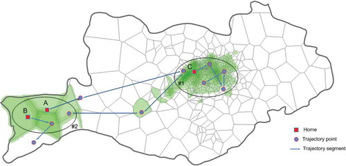
Figure 9. Trajectory distributions of urban residents and suburban residents for the five dual-centred communities. The left and right columns illustrate trajectory distributions of dual-centred community residents who live in urban and suburban area, respectively. Each row in sequence corresponds to a community in Figure 4 in the alphabetical order. Trajectories of individuals living in urban centre are distributed generally around the urban district while trajectories of persons in suburbs are distributed in both urban district and suburbs.

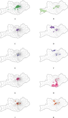
With the comparisons between trajectory distribution of urban residents and suburban residents, we discover that home–work-separate persons living in different centres possess entirely dissimilar mobility patterns (Figure 9). Trajectories of persons in urban centre are distributed generally around the urban district while trajectories of persons in suburbs are distributed in both urban district and suburbs. Figure 9 also demonstrates that home–work-separate persons living in the suburbs commute between suburban and urban district frequently. This kind of movements brings these people to have more spatial interaction with people in both urban district and suburbs, and also provides them more opportunities to form relationship with people in both centres. Commute trips and social ties between people in two centres influence each other. Due to the commute between urban and suburban areas, people in the two centres have more opportunities to meet and know each other and, consequently, make a relatively large number of mobile phone calls. On the other hand, friends between two centres lead to more movements from one centre to another. The result not only supports our conjecture that the home–work separation contributes to the formation of dual-centred communities, but also shows the importance of home–work-separate persons living in the suburbs. We thus name people who live in suburban centres while working in urban centres as ‘bridge residents’, considering their important social function in connecting separate parts when forming the community.

Given that the communities are detected based on a virtual social communication network, the fundamental reason in forming a dual-centred community is the calling connections between urban centre and suburban centre. To verify whether the home–work separation in physical space is the dominant contributor in generating calling connections between two centres, we examine all connections between two centres in dual-centred communities and take the dual-centred community A as an example to demonstrate its statistics. From community A, we identify 12107 mobile phone calls between the urban centre and the suburban centre. Among them, 14.2% of calling connections are made by ‘bridge residents’ while these people only cover 3.2% of all users living in suburban centre. Considering the complexity of social networks, people may construct connections with others because of many kinds of social activities in addition to work. Although we cannot exactly tell which type of social activities lead to the dual-centred pattern, the home–work separation plays an important role in creating the two separate centres given that small proportion of bridge residents make a relatively large number of calls. These people serve a bridge role to connect urban area and suburban area in both physical space and virtual space. The active commuting behaviours of bridge residents bring many connections between two centres. To further examine the impacts of commuting behaviour on linking two centres, we choose only suburban residents with commuting frequency greater than 10. Even though these people occupy only 34.1% of all suburban people, they generate 71.3% connecting calls. This suggests that commute travel of people living in suburban centre is a more important contributor in forming a dual-centred community. We also get similar results from the other dual-centred communities.

4.2. Temporally trajectory centre changes of bridge residents

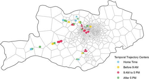
According to Section 4.1, the trajectory distributions of suburban residents (Figure 9) illustrate the connect function of bridge residents spatially, but more evidence are in need to demonstrate that the connect function is a result of their commute travel. We calculate temporally average centre position of bridge residents in each dual-centred community to provide further temporal illustration that the home–work separation is an important force in the formation of the dual-centred structure. The centres of all bridge residents are hourly calculated between 6 am and 10 pm. People are considered at home in the night-time hours, so the average positions in those hours are calculated only once for simplicity. The result illustrates that during work hours (9 am–5 pm), the centres of bridge residents are concentrated in the realm of the centres with some random vibration caused by different hourly calling frequencies. Before 9 am, the centres are moving from suburban centres towards the urban centres; while after 5 pm, the centres are moving in the opposite direction (Figure 10). The moving pattern of the centres corresponds to the commuting rhythm of residents, indicating the connect function of the bridge residents from the temporal perspective. To conclude, both the spatial and temporal travel patterns of residents support our hypothesis that the formation of dual-centred communities are greatly influenced by commuting behaviours of people, especially that of home–work-separate residents.

Figure 10. Temporal trajectory centres of bridge residents in each dual-centred community (represented by different symbols). Only the centre points at odd hours are shown for clarity. Bridge residents are referred to residents who live in suburban centres while working in urban centres. The temporal trajectory centres demonstrate that the forming of dual-centred communities is strongly influenced by the commuting behaviours of those bridge residents.

5. Conclusions

Mobile phone data-sets have served as a novel source for understanding human mobility and social network interaction. Most research has adopted community detection methods to study network structure from an aggregate level. In this research, we first adopt a community detection algorithm to extract social communities at the individual level. Then we investigate spatial patterns and characteristics of human mobility at the social community level. Spatial distributions of communities are visualized using a kernel density map approach, from which we distinguish three types of community patterns: single-centred pattern, dual-centred pattern and zonal pattern. It is interesting that the social communities exhibit the characteristic of spatially connected regions, even though partitioning a mobile social network does not take into account any geographical constraints. This finding indicates that people tend to communicate with individuals nearby. We suggest that the distance decay effect along with social phenomena such as the home–work separation contribute to several distribution patterns of social community.

In terms of human mobility patterns, we adopt angle and ROG distributions to compare trajectory characteristics among people from different communities. The major directions of communities are similar with those of the angle distribution because people would be more likely to contact each other within their communities. For ROG distributions, more users in dual-centred communities have large ROG, while the small single-centred community has the lowest proportion of people with a large ROG.

Additionally, for communities with the dual-centred pattern, we analyse the spatial distribution of home–work-separate residents’ trajectories and discover that trajectories of persons living in urban centre are distributed generally around the urban district while those living in suburbs are distributed in both urban district and suburbs. Together with the temporal travel patterns of residents, we verify our hypothesis that the forming of dual-centred communities is greatly influenced by commuting behaviours of people living in suburban area, especially that of bridge residents.

Human mobility pattern has become a hot research topic, with the support of big geospatial data. Most existing research extracts patterns from an entire population, although González, Hidalgo, and Barabási (2008) have pointed out that population heterogeneity is an essential factor in shaping the observed human mobility patterns. It is natural that different people with various travel demands will exhibit different patterns. There are some attempts to divide individuals or movements according to demographical properties (Yuan, Raubal, and Liu 2012) or travel demands (Wu et al. 2014). This research presents a novel way to group people by utilizing the communication information in mobile phone data. The results are convincing, since each group does have its special but reasonable mobility pattern.

Furthermore, this research is a beginning of exploring spatial characteristic of social communities based on mobile phone data-sets. How much can mobile phone social network reflect the characteristics of social network in reality? How can these different community patterns affect traffic and socio-economic condition of cities? These questions may be answered by employing more socio-economic models and corresponding data-sets.

Additional information

Funding

This research was supported by the Natural Science Foundation of China [grant numbers 41271386 and 41428102].

References

- Brockmann, D., L. Hufnagel, and T. Geisel. 2006. “The Scaling Laws of Human Travel.” Nature 439: 462–465. doi:10.1038/nature04292.
- Clauset, A., M. E. J. Newman, and C. Moore. 2004. “Finding Community Structure in Very Large Networks.” Physical Review E 70: 066111. doi:10.1103/PhysRevE.70.066111.
- De Montis, A., S. Caschili, and A. Chessa. 2013. “Commuter Networks and Community Detection: A Method for Planning Sub Regional Areas.” The European Physical Journal Special Topics 215: 75–91. doi:10.1140/epjst/e2013-01716-4.
- Eagle, N., Y. de Montjoye, and L. M. Bettencourt. 2009. “Community Computing: Comparisons between Rural and Urban Societies Using Mobile Phone Data.” In International Conference on Computational Science and Engineering, 2009. CSE’09, 144–150. Vancouver, BC: IEEE.
- Eagle, N., M. Macy, and R. Claxton. 2010. “Network Diversity and Economic Development.” Science 328: 1029–1031. doi:10.1126/science.1186605.
- Eagle, N., A. S. Pentland, and D. Lazer. 2009. “Inferring Friendship Network Structure by Using Mobile Phone Data.” Proceedings of the National Academy of Sciences of the United States of America 106: 15274–15278. doi:10.1073/pnas.0900282106.
- Erdős, P., and A. Rényi. 1960. “On the Evolution of Random Graphs.” Publications of the Mathematical Institute of the Hungarian Academy of Sciences 5: 17–61.
- Gao, S., Y. Liu, Y. Wang, and X. Ma. 2013. “Discovering Spatial Interaction Communities from Mobile Phone Data.” Transactions in GIS 17 (3): 463–481. doi:10.1111/tgis.12042.
- Girvan, M., and M. E. Newman. 2002. “Community Structure in Social and Biological Networks.” Proceedings of the National Academy of Sciences of the United States of America 99: 7821–7826. doi:10.1073/pnas.122653799.
- González, M. C., C. A. Hidalgo, and A.-L. Barabási. 2008. “Understanding Individual Human Mobility Patterns.” Nature 453: 779–782. doi:10.1038/nature06958.
- Granovetter, M. S. 1973. “The Strength of Weak Ties.” American Journal of Sociology 1360–1380. doi:10.1086/225469.
- Hagel, J. 1999. “Net Gain: Expanding Markets through Virtual Communities.” Journal of Interactive Marketing 13: 55–65. doi:10.1002/(SICI)1520-6653(199924)13:1<55::AID-DIR5>3.0.CO;2-C.
- Hidalgo, C. A., and C. Rodriguez-Sickert. 2008. “The Dynamics of a Mobile Phone Network.” Physica A: Statistical Mechanics and its Applications 387: 3017–3024. doi:10.1016/j.physa.2008.01.073.
- Kang, C., Y. Liu, X. Ma, and L. Wu. 2012. “Towards Estimating Urban Population Distributions from Mobile Call Data.” Journal of Urban Technology 19: 3–21. doi:10.1080/10630732.2012.715479.
- Kang, C., S. Sobolevsky, Y. Liu, and C. Ratti. 2013. “Exploring Human Movements in Singapore: A Comparative Analysis Based on Mobile Phone and Taxicab Usages.” In Proceedings of the 2nd ACM SIGKDD International Workshop on Urban Computing, No. 1. New York: ACM.
- Krings, G., F. Calabrese, C. Ratti, and V. D. Blondel. 2009. “Scaling Behaviors in the Communication Network between Cities.” In International Conference on Computational Science and Engineering, 2009. CSE’09, 936–939. Vancouver, BC: IEEE.
- Lambiotte, R., V. D. Blondel, C. de Kerchove, E. Huens, C. Prieur, Z. Smoreda, and P. Van Dooren. 2008. “Geographical Dispersal of Mobile Communication Networks.” Physica A: Statistical Mechanics and its Applications 387 (21): 5317–5325. doi:10.1016/j.physa.2008.05.014.
- Liu, Y., Z. Sui, C. Kang, and Y. Gao. 2014. “Uncovering Patterns of Inter-Urban Trip and Spatial Interaction from Social Media Check-In Data.” PLoS ONE 9 (1): e86026. doi:10.1371/journal.pone.0086026.
- Newman, M. E., and M. Girvan. 2004. “Finding and Evaluating Community Structure in Networks.” Physical Review E 69: 026113. doi:10.1103/PhysRevE.69.026113.
- Onnela, J. P., S. Arbesman, M. C. González, A. L. Barabási, and N. A. Christakis. 2011. “Geographic Constraints on Social Network Groups.” PLoS ONE 6: e16939. doi:10.1371/journal.pone.0016939.
- Onnela, J.-P., J. Saramäki, J. Hyvönen, G. Szabó, D. Lazer, K. Kaski, J. Kertész, and A.-L. Barabási. 2007. “Structure and Tie Strengths in Mobile Communication Networks.” Proceedings of the National Academy of Sciences of the United States of America 104: 7332–7336. doi:10.1073/pnas.0610245104.
- Palla, G., A.-L. Barabási, and T. Vicsek. 2007. “Quantifying Social Group Evolution.” Nature 446: 664–667. doi:10.1038/nature05670.
- Pfaff, J. 2010. “Mobile Phone Geographies.” Geography Compass 4: 1433–1447. doi:10.1111/j.1749-8198.2010.00388.x.
- Phithakkitnukoon, S., Z. Smoreda, and P. Olivier. 2012. “Socio-Geography of Human Mobility: A Study Using Longitudinal Mobile Phone Data.” PloS ONE 7: e39253. doi:10.1371/journal.pone.0039253.
- Poston, D. L. 1972. “Socioeconomic Status and Work-Residence Separation in Metropolitan America.” The Pacific Sociological Review 15: 367–380. doi:10.2307/1388353.
- Ratti, C., S. Sobolevsky, F. Calabrese, C. Andris, J. Reades, M. Martino, R. Claxton, and S. H. Strogatz. 2010. “Redrawing the Map of Great Britain from a Network of Human Interactions.” PLoS ONE 5: e14248. doi:10.1371/journal.pone.0014248.
- Schnore, L. F. 1954. “The Separation of Home and Work: A Problem for Human Ecology.” Social Forces 32: 336–343. doi:10.2307/2574115.
- Song, C., T. Koren, P. Wang, and A.-L. Barabási. 2010. “Modelling the Scaling Properties of Human Mobility.” Nature Physics 6: 818–823. doi:10.1038/nphys1760.
- Song, C., Z. Qu, N. Blumm, and A.-L. Barabási. 2010. “Limits of Predictability in Human Mobility.” Science 327: 1018–1021. doi:10.1126/science.1177170.
- Thiemann, C., F. Theis, D. Grady, R. Brune, and D. Brockmann. 2010. “The Structure of Borders in a Small World.” PloS ONE 5: e15422. doi:10.1371/journal.pone.0015422.
- Tobler, W. R. 1970. “A Computer Movie Simulating Urban Growth in the Detroit Region.” Economic Geography: 234–240. doi:10.2307/143141.
- Wellman, B. 1999. “The Network Community: An Introduction.” In Networks in the Global Village, edited by B. Wellman, 1–48. Boulder, CO: Westview.
- Wellman, B., and S. Wortley. 1990. “Different Strokes from Different Folks: Community Ties and Social Support.” American Journal of Sociology 96: 558–588. doi:10.1086/229572.
- Wu, L., Y. Zhi, Z. Sui, and Y. Liu. 2014. “Intra-Urban Human Mobility and Activity Transition: Evidence from Social Media Check-In Data.” PLoS ONE 9 (5): e97010. doi:10.1371/journal.pone.0097010.
- Yuan, Y., M. Raubal, and Y. Liu. 2012. “Correlating Mobile Phone Usage and Travel Behavior – A Case Study of Harbin, China.” Computers, Environment and Urban Systems 36 (2): 118–130. doi:10.1016/j.compenvurbsys.2011.07.003.