Sandwich mapping of diseases with a small sample in a stratified heterogeneous domain

Abstract

The error associated with the mapping of a disease is determined based on the sampling triple: the properties of the disease, the way of sampling and the methods used for mapping. The Kriging method projects the best linear unbiased disease map if the disease data have both spatial autocorrelation (SAC) and second-order stationarity. The Kriging method fails if SAC is null or weak. For such a situation, the sandwich interpolation method is applicable if the disease shows stratified heterogeneity in a space. The sandwich mapping comprises three steps: the domain is stratified based on the principle of minimizing variance within strata and maximizing variance between strata; the prevalence value and its variance within a stratum are estimated; and lastly, the quantities of strata are transformed into the reporting units.

Keywords:

• disease mapping
• small sample
• spatial stratified heterogeneity
• sandwich mapping

1. Introduction

In disease mapping, it is often needed to show how disease risk varies in relation to geographical space by projecting sample data to unsampled sites based on the statistical properties of the data and the space to be modelled. The prevalence of a disease is often spatially autocorrelated and heterogeneous (Haining 2003; Christakos 2005; Wang et al. 2012). These properties would make the use of conventional statistics inefficient or even biased. However, they would also provide opportunities for disease mapping based on small samples (Haining 2003; Griffith 2005; Wang, Haining, and Cao 2010a).

The existence of spatial autocorrelation (SAC) allows a single data point to represent the range of values in an area, and this convenient parsimony of representation increases (Rodriguez-Iturbe and Mejia, 1974; Haining 1988; Shi 2010; Griffith 2005; Wang, Hu, et al. 2013) and optimizes (Matheron 1963; Goovaerts 1997; Wang et al., 2009, 2011; Wang, Haining, et al. 2013; Wang, Jiang, et al. 2013; Hu and Wang 2011) the efficiency of mapping. The mapping methods explicitly or implicitly based on SAC include, e.g., Kriging, inverse distance weighted (IDW) interpolation, spatial spline regressions and Thiessen polygons. SAC is tested with Moran’s I (Moran 1950) for regional data, such as data recorded in administrative units, and with a semivariogram for spatially continuous data, such as temperature across an area. When the data have both SAC and second-order stationarity, the Kriging method can perform a best linear unbiased estimate (BLUE) mapping. These mapping approaches fail if SAC is null or weak. For such a situation, the sandwich mapping (Wang, Haining, et al. 2013) is applicable if the disease data have stratified heterogeneity.

We describe stratified heterogeneity and sandwich mapping in Section 2. I illustrate these concepts and approaches using two empirical examples in Section 3. We furnish a discussion and formulate conclusions in Section 4.

2. Stratified heterogeneity and sandwich mapping

Heterogeneous is a term used in statistics to indicate the inequality of some quantity of interest (usually a variance) in a number of different groups, populations, etc. (Everitt 2002, p. 178). Spatial heterogeneity refers to the uneven distribution of a trait, event or relationship across a region (Anselin 2010). Spatial heterogeneity is usually measured with the Local Indicators of Spatial Association (Anselin 1995), Gi (Getis and Ord 1992) or semivariogram techniques. In addition to the heterogeneity measured based on individual sample subjects, there is also heterogeneity among groups of sample subjects, e.g., differences in a certain characteristic between climate zones or between watersheds. In this paper, I call such a group a stratum, and use the term stratified heterogeneity to refer to the difference between strata and the relative homogeneity within a stratum. Stratified heterogeneity is a key concept in sandwich mapping.

2.1. Stratified heterogeneity

In sandwich mapping, a stratum is an area where the population is relatively homogeneous, and thus the population can be represented by a small sample (Li et al. 2008; Fischer and Wang 2011). The stratification of a population can be achieved using an index termed as the geographical detector. The value of this index is (Wang et al. 2010b; Wang and Hu 2012)

where s² and s_z² are variance of the prevalence of a disease in the study area and in stratum z, respectively, z = 1, 2, …, L; W_z = n_z/n, and n_z and n denote the numbers of random sample elements in stratum z and in the study area, respectively; p and p_z are prevalence of a disease in the study area and in stratum z, respectively; the value of q has been proved to be within [0,1]; it is 0 if the variances within and between strata are not different, suggesting that there is no stratified heterogeneity, and it is 1 if the variance within each stratum is zero, suggesting that there is a perfect stratified heterogeneity. The stratification in sandwich mapping is done to partition the study area through maximizing q.

2.2. Sandwich mapping

If a disease has stratified heterogeneity, its prevalence in a stratum can be estimated using stratification statistics (Cochran 1977). The result of the estimation can then be used for mapping through areal interpolation or sandwich interpolation. An areal interpolation can be used to map areal values (Goodchild, Anselin, and Deichmann 1993), and a sandwich interpolation can be used to map both the areal values and their variances (Wang, Haining, et al. 2013). Figure 1 illustrates the mechanism of sandwich mapping, which comprises three steps.

Figure 1. Mechanism of sandwich mapping (Wang, Haining, et al. 2013, permitted by www.pion.co.uk and www.envplan.com).

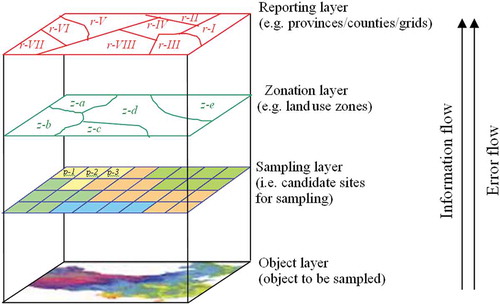
Step 1. Stratification of a disease. A disease area is stratified according to the principle of minimizing the within-stratum variance and maximizing the across-strata variance (the zonation layer in Figure 1). There are numerous algorithms, e.g., k-means and self-organizing maps (SOMs), for the classification of the data at an interval-ratio scale (Cao et al. 2013). Notably, stratification can even be achieved manually based on expert knowledge (Wang et al. 2002). Li et al. (2008) provide a review of different approaches to stratification or classification.

Step 2. Estimating disease prevalence within a stratum. The disease prevalence p_z of stratum z and its variance are calculated as

(1)

(2)

Step 3. Estimating disease prevalence for reporting units. The reporting units are the areal units in the final disease map. They can be administrative units, grids, physical units (e.g., watersheds), or any polygons of interest (the reporting layer in Figure 1). To transform the values from the strata to the reporting units, first of all, the strata are overlaid with the reporting units. A reporting unit might intersect with one or several strata. The mean and its variance in each reporting unit are then estimated using the stratified statistics as follows:

(3)

(4)

where r = 1, …, M, and M is the number of reporting units; L_r is the number of strata intersecting with reporting unit r; and W_r∩z/r is the proportion of population in stratum z enclosed by reporting unit r. Notably, the disease prevalence and its variance for a reporting unit can be estimated in this way, even if there are no sample subjects inside the reporting unit, because the values of the reporting unit are estimated according to the intersected strata, not directly based on the sample.

3. Two empirical examples

Many diseases are transmitted through disease vectors, such as rodents, mosquitoes and snails, whose distributions are strongly controlled by land use. Land use typically has spatially stratified heterogeneity. Here, we illustrate the sandwich approach to mapping cultivated land in Shandong province, China. We also compared the error of our mapping with those of several mainstream methods. Among these methods, the simple averaging of the sample is a basic estimator, with no effort to address spatial variation; Block Kriging weights a sample and minimizes the error variance under an unbiased restriction; its performance is proportional to the strength of the SAC; the hierarchical Bayesian estimator considers SAC as its prior, with accompanying covariance, and the performance of this method is limited if the prior and covariance are weak or are not well identified.

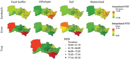
The true values of the cultivated land area were acquired from aerial remote-sensing images, with 0.2 × 0.2 m² spatial resolution, covering the entire province. A sample with a 0.5% sampling rate was randomly drawn from the true map. Sandwich and several other methods were employed to draw maps using small samples, reporting on three spatial scales, namely watersheds, prefectures and grid (Figure 2). The errors were measured as the difference between the maps and the true values, as shown in Figure 3. Clearly, sandwich mapping has the smallest error among the methods because the cultivated land area in Shandong province has spatially stratified heterogeneity, whereas the SAC is weak, and therefore the Kriging method performs poorly. Sandwich mapping appears to be the most appropriate method for these data. The second example is the mapping of neural tube defect (NTD) of birth in Heshun county, China, using the sandwich mapping method. Some environmental factors are highly suspected to have contributed to the occurrence of the disease in the study county, see Figure 4 (Wang et al. 2010b). The NTD prevalence and its variance in each of 10 watersheds are calculated by a stratified small sample using Equations (1) and (2), respectively. The values are then input into Equations (3) and (4) to estimate the NTD prevalence and its variance in each of the nine administrative reporting units. We went through the same process for the environmental factors, including fault buffers, lithotypes and soil types. The prevalence and their absolute errors from the true map are presented in Figure 4. Clearly, the error of sandwich mapping is determined by the degree of the spatially stratified heterogeneity of the disease or its determinants, proxied by the environmental factors.

Figure 2. Mapping cultivated land area in Shandong province, China (modified, Wang, Haining, et al. 2013, permitted by www.pion.co.uk and www.envplan.com).

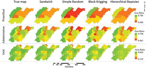
Figure 3. Error of the mapping of the cultivated land area in Shandong province, China (modified, Wang, Haining, et al. 2013, permitted by www.pion.co.uk and www.envplan.com).

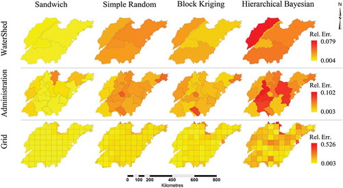
Figure 4. Sandwich mapping of NTD prevalence in Heshun county, China.

4. Conclusion and discussion

Kriging is the most common mapping method for a spatially autocorrelated target with second-order stationarity. Kriging performs poorly or inefficiently if SAC is absent. In this situation, the sandwich method offers an alternative approach for mapping when the target has stratified heterogeneity.

The determination of strata is critical in applying sandwich mapping, but determining the strata can be challenging. Failing to identify the strata or the absence of a stratified structure can undermine the utility of sandwich mapping.

As is the case for SAC, stratified heterogeneity does not always exist. Just like a semivariogram is critical to ensure the efficiency of Kriging, stratification or classification, measured by the q-statistic, is also important for the sandwich estimator. The greater the stratified heterogeneity, the more precise the sandwich mapping. The zonal structure may be defined by the variables that are correlated to the estimates, or formed through post-stratification after selection of the sample (Cochran 1977, p. 134). Therefore, stratification does not necessarily have to be in the geographical space; it can also be in any other space.

In summary, Kriging performs well if SAC is strong, and the sandwich estimator performs well if stratified heterogeneity is strong. Determining an exact threshold for use in switching between the two methods is currently under study.

Disclosure statement

No potential conflict of interest was reported by the author.

Acknowledgement

I appreciate Xun Shi, reviewers and editors of the journal for improving this manuscript.

Additional information

Funding

This study was supported by National Basic Research Program of China (973 Program) [grant number 2012CB955503]; and NSFC [41023010], [41271404].

References

- Anselin, L. 1995. “Local Indicators of Spatial Association – LISA.” Geographical Analysis 27 (2): 93–115. doi:10.1111/j.1538-4632.1995.tb00338.x.
- Anselin, L. 2010. “Thirty Years of Spatial Econometrics.” Papers in Regional Science 89 (1): 3–25. doi:10.1111/j.1435-5957.2010.00279.x.
- Cao, F., Y. Ge, and J. F. Wang. 2013. “Optimal Discretization for Geographical Detectors-Based Risk Assessment.” GIScience & Remote Sensing 50 (1): 78–92.
- Christakos, G. 2005. Random Field Models in Earth Sciences. New York, NY: Dover Publications.
- Cochran, W. G. 1977. Sampling Techniques. 3rd ed. New York, NY: John Wiley & Sons.
- Everitt, B. S. 2002. The Cambridge Dictionary of Statistics. 2nd ed. Cambridge: Cambridge University Press.
- Fischer, M. M., and J. F. Wang. 2011. Spatial Data Analysis: Problems, Techniques and Applications. Berlin: Springer.
- Getis, A., and J. K. Ord. 1992. “The Analysis of Spatial Association by Use of Distance Statistics.” Geographical Analysis 24 (3): 189–206. doi:10.1111/j.1538-4632.1992.tb00261.x.
- Goodchild, M. F., L. Anselin, and U. Deichmann. 1993. “A Framework for the Areal Interpolation of Socioeconomic Data.” Environment and Planning A 25: 383–397. doi:10.1068/a250383.
- Goovaerts, P. 1997. Geostatistics for Natural Resources Evaluation. Oxford: Oxford University Press.
- Griffith, D. A. 2005. “Effective Geographic Sample Size in the Presence of Spatial Autocorrelation.” Annals of the Association of American Geographers 95: 740–760. doi:10.1111/j.1467-8306.2005.00484.x.
- Haining, R. P. 1988. “Estimating Spatial Means with an Application to Remotely Sensed Data.” Communications in Statistics - Theory and Methods 17: 573–597. doi:10.1080/03610928808829641.
- Haining, R. P. 2003. Spatial Data Analysis: Theory and Practice. Cambridge: Cambridge University Press.
- Hu, M.-G., and J.-F. Wang. 2011. “A Spatial Sampling Optimization Package Using MSN Theory.” Environmental Modelling & Software 26 (4): 546–548. doi:10.1016/j.envsoft.2010.10.006.
- Li, L. F., J. F. Wang, Z. D. Cao, and E. Zhong. 2008. “An Information-Fusion Method to Identify Pattern of Spatial Heterogeneity for Improving the Accuracy of Estimation.” Stochastic Environmental Research and Risk Assessment 22 (6): 689–704. doi:10.1007/s00477-007-0179-1.
- Matheron, G. 1963. “Principles of Geostatistics.” Economic Geology 58: 1246–1266. doi:10.2113/gsecongeo.58.8.1246.
- Moran, P. A. P. 1950. “Notes on Continuous Stochastic Phenomena.” Biometrika 37: 17–23. doi:10.1093/biomet/37.1-2.17.
- Rodríguez-Iturbe, I., and J. M. Mejía. 1974. “The Design of Rainfall Networks in Time and Space.” Water Resources Research 10: 713–728. doi:10.1029/WR010i004p00713.
- Shi, X. 2010. “Selection of Bandwidth Type and Adjustment Side in Kernel Density Estimation over Inhomogeneous Backgrounds.” International Journal of Geographical Information Science 24 (5): 643–660. doi:10.1080/13658810902950625.
- Wang, J. F., G. Christakos, and M. G. Hu. 2009. “Modeling Spatial Means of Surfaces with Stratified Nonhomogeneity.” IEEE Transactions on Geoscience and Remote Sensing 47 (12): 4167–4174. doi:10.1109/TGRS.2009.2023326.
- Wang, J. F., R. Haining, and Z. D. Cao. 2010a. “Sample Surveying to Estimate the Mean of a Heterogeneous Surface: Reducing the Error Variance through Zoning.” International Journal of Geographical Information Science 24 (4): 523–543. doi:10.1080/13658810902873512.
- Wang, J.-F., R. Haining, T.-J. Liu, L.-F. Li, and C.-S. Jiang. 2013. “Sandwich Estimation for Multi-Unit Reporting on a Stratified Heterogeneous Surface.” Environment and Planning A 45 (10): 2515–2534. doi:10.1068/a44710.
- Wang, J.-F., M.-G. Hu, C.-D. Xu, G. Christakos, Y. Zhao, and J. A. Añel. 2013. “Estimation of Citywide Air Pollution in Beijing.” PLoS ONE 8 (1): e53400. doi:10.1371/journal.pone.0053400.
- Wang, J.-F., and Y. Hu. 2012. “Environmental Health Risk Detection with Geogdetector.” Environmental Modelling & Software 33: 114–115. doi:10.1016/j.envsoft.2012.01.015.
- Wang, J.-F., C.-S. Jiang, M.-G. Hu, Z.-D. Cao, Y.-S. Guo, L.-F. Li, T.-J. Liu, and B. Meng. 2013. “Design-Based Spatial Sampling: Theory and Implementation.” Environmental Modelling & Software 40: 280–288. doi:10.1016/j.envsoft.2012.09.015.
- Wang, J.-F., X.-H. Li, G. Christakos, Y.-L. Liao, T. Zhang, X. Gu, and X.-Y. Zheng. 2010b. “Geographical Detectors-Based Health Risk Assessment and Its Application in the Neural Tube Defects Study of the Heshun Region, China.” International Journal of Geographical Information Science 24 (1): 107–127. doi:10.1080/13658810802443457.
- Wang, J. F., J. Y. Liu, D. F. Zhuan, L. F. Li, and Y. Ge. 2002. “Spatial Sampling Design for Monitoring the Area of Cultivated Land.” International Journal of Remote Sensing 23 (2): 263–284. doi:10.1080/01431160010025998.
- Wang, J.-F., B. Y. Reis, M.-G. Hu, G. Christakos, W.-Z. Yang, Q. Sun, Z.-J. Li, et al. 2011. “Area Disease Estimation Based on Sentinel Hospital Records.” PLoS ONE 6 (8): e23428. doi:10.1371/journal.pone.0023428.
- Wang, J.-F., A. Stein, B.-B. Gao, and Y. Ge. 2012. “A Review of Spatial Sampling.” Spatial Statistics 2 (1): 1–14. doi:10.1016/j.spasta.2012.08.001.