Conceptually categorizing geographic features from text based on latent semantic analysis and ontologies

ABSTRACT

Categorizing geographic features from text is a process of assigning a collection of text documents that describe geographic features to predefined categories. This paper presents a new approach to categorize geographic features from text that begins at the level of the individual document. Using latent semantic analysis, similar geographic features are grouped into predefined categories through capturing the semantic context of text. By incorporating ontologies into latent semantic analysis, the domain knowledge can be incorporated into the categorizing process. The proposed approach can allocate each geographic feature into more than one category and is able to identify a set of key concepts to represent each category. The results from an experimental evaluation using the proposed approach showed promise in categorizing geographic features from text.

KEYWORDS:

• Text classification
• ontology
• geographic features
• latent semantic analysis

1. Introduction

Categorizing geographic features from text is a process of assigning geographic features (e.g. mountains) from text to a set of predefined categories. This process plays an important role in geographic information retrieval and mining. However, to date, little attention has been paid to this research area. Most studies have focused on integration and formalization of existing geographic categorizations (Kavouras and Kokla 2002; Kuhn 2002; Comber, Lear, and Wadsworth 2010; Bian and Hu 2007).

Categorizing geographic features from text documents into predefined categories is a challenge (Smith and Mark 2001). Predefined categories are often available for geographic features, the results however tend to vary based on different applications. Moreover, humans usually carry out this task and their subjectivity in categorization presents a problem: for the same collection of text documents, different people might give different categorization results. In recent years, a number of methods for text document categorization have been developed. They might be directly applied to geographic features; however, there are some difficulties.

First, text document categorization approaches usually follow an approach that involves the division of a set of text documents into subcategories. The categories that result from this division are mutually exclusive, that is, there is no overlap between mutually exclusive categories, and each document belongs to one and only one category. Geographic features are spatial features on or near the surface of the earth, and they are typically complex. Overlapping categories are common to geographic features, and each feature may be assigned to multiple categories (Usery 1993, 1996; Mark, Smith, and Tversky 1999; Smith and Mark 2003). For example, mountains generally occupy particular regions of the earth’s surface, and they may be associated with more than one type of land cover. Thus, a mountain might be associated with more than one category if land cover is used to categorize mountains.

Second, synonymy and polysemy have been a challenge in handling text documents, including geographic feature documents (Baharudin, Lee, and Khan 2010). Synonymy refers to the existence of different words with almost identical or similar meanings, while polysemy refers to the fact that some words have multiple and unrelated meanings. A failure to account for synonymy can lead to many small and disjointed categories, while the failure to account for polysemy might lead to categorizing unrelated documents (Kobayashi and Aono 2006). Last but not least, text documents that describe geographic features often contain a great deal of domain knowledge such as domain-specific terminologies (Goldberg, Wilson, and Knoblock 2009). Capturing these terminologies and incorporating the prior domain knowledge will facilitate geographic feature categorization. Most existing methods, however, are based on invariant domain knowledge (Zheng, Borchert, and Jiang 2010).

To address these issues, this paper explores a novel approach to categorizing geographic features from text. This approach begins at the level of the individual documents. Similar documents that describe geographic features are assigned to the same category based on the semantic mapping of terms in two groups. One group consists of the terms extracted from the documents and they are used to present geographic features. The bag-of-words model, a simplifying representation that is commonly used in natural language processing and information retrieval, is adopted in this paper to process the documents. However, instead of using the frequency of occurrence of each word or term frequency, this paper used term frequency-inverse document frequency (TF-IDF), a most popular method to weight terms in both information retrieval and text classification. The other group consists of the terms that are used to present predefined categories. The semantic context of terms is captured using latent semantic analysis (LSA), a statistic method to extract and represent the contextual-usage meaning of words (Deerwester et al. 1990; Landauer and Dumais 1997). The categorizing process is driven by domain knowledge through ontologies to control extraction of terms from text and to specify terms to represent the predefined categories. By incorporating ontologies into LSA, the proposed approach allows to allocate each geographic feature into more than one category and to identify a set of key concepts for each category as well.

In this paper, the performance of the proposed approach was evaluated by assigning a set of mountains into one or more predefined categories from a collection of text documents. We have chosen an experimental evaluation approach because of the very nature of the task – automatic text categorization heavily relies on the collection of text documents (Sebastiani 2002). The results showed promise in categorizing geographic features from text.

This paper extends a previous study by incorporating domain knowledge into LSA for geographic feature categorization (Huang 2011). The remainder of the paper is organized as follows. First, in Section 2, we examine related work in text document categorization, followed by a brief introduction to LSA in Section 3. We then outline our proposed approach including a step-by-step walk-through example in Section 4. To our knowledge, LSA has not been thoroughly examined for the geographic information science (GIS) community. This detailed example can serve to introduce the community to a technique that they may not have encountered. In Section 5, we present an experimental evaluation on a particular region in New Mexico, USA. The evaluation and discussion focus on varying various parameters, which are the important aspects of the proposed approach. Finally, in Section 6, we conclude by highlighting some implications and limitations of the approach. In addition, we offer suggestions for future studies.

2. Related work

Text document categorization is an important area of text mining and information retrieval. In recent years, a number of methods have been discussed in the literature. Among them, K-means is a simple but effective method of assigning documents into k mutually exclusive categories by using an iterative algorithm. This method minimizes the sum of distances from each document to its category centroid. Other methods are based on advanced machine learning and information retrieval methods, such as support vector machines (Kumar and Gopal 2010), Bayesian probabilistic methods (Nunzio 2009), neural networks (Yu, Xu, and Li 2008), genetic algorithms (Uguz 2011) and latent semantic indexing (Wei, Yang, and Lin 2008). Most of these methods begin at the level of the entire set of documents (namely, at the level of the population) and then divide the documents into categories. This approach is often treated as a ‘black-box’ and easy to manipulate. Moreover, using this approach, each document is usually assigned to a single category. However, a document is often associated with more than one category (Hearst 1999). An alternative strategy is to begin at the level of individual documents (namely, at the level of the instances) and then group individual documents into categories. In this way, a document can be allocated to more than one category (Duckham and Worboys 2005; Odgers, McBratney, and Minasny 2011). Furthermore, most text document categorization methods assign documents into categories solely based on a numerical measure of similarities between documents. The obtained set of categories can be well defined mathematically. However, they may not have a meaningful conceptual interpretation if domain knowledge is not taken into account. To overcome this limitation, conceptual clustering was proposed to use a set of concepts to describe each category (Michalski 1980; Fisher 1987). The concepts can be obtained from a predefined set of concepts based on domain terminologies, or they can be automatically derived from text documents.

Last, ontology, an important resource for text document categorization, is often used to represent document knowledge. An ontology is a formal explicit specification of a shared conceptualization of a domain of interest (Gruber 1993). A set of concepts and the relationships between them are the two main components in an ontology (Guarino 1998). Recently, ontologies have been integrated into the process of categorizing text documents. For instance, Srinivasan (2001) used medical subject heading (MeSH) terms to mine the metadata of MEDLINE documents in order to yield high-level summaries. Song and Park (2009) proposed a genetic algorithm for text categorization using ontologies. Zheng, Borchert, and Jiang (2010) developed a key concept induction algorithm to identify key concepts and classify medical documents based on ontologies. In most existing methods, however, the use of ontologies is limited to the extraction of terms from text documents. In other words, similar to a domain dictionary, ontologies are only served as a control group to extract terms from text documents based on the concepts specified in the ontologies. The use of ontologies has not been fully examined in text document categorization.

Text mining from geographic information is an active research topic in GIS and computer science. Existing research focuses on, for example, identifying patterns in spatial information (Wise et al. 1995), finding and extracting geographic references within text (Rauch, Bukatin, and Baker 2003; Lieberman et al. 2007) and integrating semantics of geographic categories (Kuhn 2002). However, categorizing geographic features from text documents has not yet been explored sufficiently.

3. Latent semantic analysis

LSA takes the input of an m × n term-document matrix X, where the matrix rows m correspond to terms, namely words that occur in a document, and the columns n to documents. The matrix X represents the importance (namely, the weights) of terms to documents. Although there are some variations, LSA involves three common processes, namely, constructing a term-document matrix, projecting both documents and terms onto a vector space and reducing the vector space. Based on singular value decomposition (SVD) and dimension reduction techniques, LSA produces three reduced matrices, namely, U_k, S_k, and V_k. The matrix U_k has a k-dimensional vector for each of the m terms, the matrix V_k has a k-dimensional vector for each of the n documents and the matrix S_k has the k singular values. Thus, the matrix X can be approximated as X_k = U_kS_kV_k^T, which is claimed as the best approximation to X of any rank-k matrix in the least squares sense.

The number of reduced dimensions (namely, the parameter k) also plays a critical role in LSA. The optimal k is determined empirically for each corpus. In general, smaller k values are preferred when using LSA due to the computational cost associated with the SVD algorithm (Zha and Simon 1998). A common way to determine the k value is through the Frobenius norm, which is defined as the square root of the sum of the absolute squares of its elements. This value is often used to measure the difference between two matrices. Given the matrix S and its Frobenius norm ||S||_F, k is defined as the minimum value that satisfies the following condition: ||S_k||_F/||S||_F ≥ p, where p is an acceptable threshold of approximation between the original matrix and its reduced matrix. Based on the generated k, the two generated matrices, U and V, are truncated to two reduced vector spaces, U_k and V_k, respectively. These two matrices project terms and documents onto the reduced k-dimensional vector space S_k, respectively.

The use of the three derived matrices, U_k, S_k and V_k, from LSA depends on applications. For example, the similarity between any two documents can be computed based on their places in the matrix of V_k. The calculated similarity value can then be used to classify documents. The similarity value can also be used for document retrieval by specifying a query, where the query is represented as a set of terms. Because the query can be treated as a single document, the similarity between the query and each document can be calculated. The documents that receive high similarity values can be considered as the relevant documents to the query. Likewise, the similarity between any two terms can be computed based on their places in the matrix of U_k. The calculated similarity value can then be used to identify keywords. For more details about LSA, including theory and applications, see Deerwester et al. (1990) and Landauer, Foltz and Laham (1998, 51).

As an automatic and objective method to analyse text through statistic methods, LSA has proven to effectively overcome synonymy and polysemy problems by capturing the semantic content of text (Landauer, Foltz, and Laham 1998). In addition to information retrieval, LSA has also been applied to many applications, such as cognitive theory (Denhiere et al. 2006) and educational applications (Millis et al. 2006). However, little work has been done on LSA for geographic information. One exception is spatialization, which is the process of generating an information display of non-spatial data (Fabrikant et al. 2004).

4. The proposed method

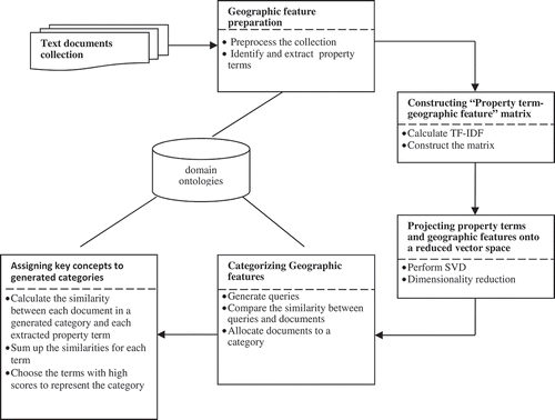
As shown in Figure 1, the proposed approach comprises five main phases: (1) geographic feature preparation, (2) constructing ‘property term–geographic feature’ matrix, (3) projecting property terms and geographic features onto a reduced vector space, (4) categorizing geographic features and (5) assigning key concepts to generated categories. Each phase is described in detail below.

Figure 1. Framework of the proposed method.

4.1. Geographic feature preparation

In this phase, first common preprocesses in a typical text classification are performed, including, for example, case folding and stop words removal. Case folding is to convert texts to lower case to avoid case sensitivity. Stop words, which are common words but do not contain significant meaning, are removed to reduce computational burden. After that, the main task is to identify and extract the terms that are used to describe geographic features (hereafter, these terms are referred to as the property terms). This process is done with the support of the corresponding domain ontologies. More specifically, concepts in a corresponding ontology are used to control the identification of the property terms. Only those that appear in the set of concepts are considered as a property term and they are extracted for further processing.

4.2. Constructing ‘property term–geographic feature’ matrix

In this phase, a term-document matrix (hereafter referred to as a ‘property term–geographic feature’ matrix) for LSA analysis is constructed. The rows of the matrix correspond to the property terms extracted from the first phase (e.g. ‘Douglas fir’ in Table 1), and columns correspond to the documents of geographic features (e.g. ‘g1’ in Table 1). The cell values in the matrix represent the weights, or importance of the property terms in geographic features. The bag-of-words model is adopted to assign the cell values. However, instead of using term frequency, the importance is represented by TF-IDF, a most popular method to weight terms in both information retrieval and text classification. The TF-IDF values are the product of two statistics, term frequency and inverse document frequency. The TF-IDF values indicate the frequency of an individual property term for one geographic feature and relative to the geographic feature collection. The importance is increased by the number of times a property term appears in a geographic feature but is offset by the frequency of the property term in the collection of geographic features. Studies show that SVD can effectively capture the co-occurrence terms when TF-IDF values are used to represent the importance of the terms in documents (Robertson 2004; Chen, Liang, and Pan 2008).

Table 1. An example: property term–geographic feature matrix.

Geographic features	Property terms
g1	Ponderosa pine, Douglas fir, white fir, blue spruce, Engelmann spruce
g2	Pinyon juniper, Gambel oak, mountain mahogany, upper Sonoran shrubs, upper Sonoran grasses, lower Sonoran shrubs, lower Sonoran grasses
g3	Semi-desert grassland, chaparral, Chihuahuan Desert scrub, mesquite, creosote bush, yucca
g4	Mesquite, creosote bush, manzanita, Chihuahuan Desert grasses, junipers, scrub oak
g5	Pinyon juniper, alligator juniper, Emory oak, Arizona white oak
g6	Pinyon juniper, oak, ponderosa pine
g7	Pinyon juniper, alligator juniper, oak, ponderosa pine, Douglas fir
g8	Pinyon juniper, Gambel oak, mountain mahogany
	g1 g2 g3 g4 g5 g6 97 g8

Rows in the 9 × 8 ‘property term–geographic feature’ matrix correspond to the 9 out of 25 property terms that appear in at least two geographic features (these terms are italicized in property terms and for the demonstration purpose only, these terms are included in the matrix). Columns correspond to the eight geographic features (g1–g8). The values in the matrix are the TF-IDF values of the property terms in the documents.

To illustrate the proposed method, we use a simple example to demonstrate its main processes. As shown in Table 1, there are 25 different extracted property terms in eight documents, one for each geographic feature. Nine out of 25 property terms appear in at least two geographic features. For the demonstration purpose, only these terms are used to construct a property term–geographic feature matrix. These nine property terms are Douglas fir, Gambel oak, alligator juniper, creosote bush, mesquite, mountain mahogany, oak, pinyon juniper and ponderosa pine. These terms are italicized in Table 1. The dimension of the constructed matrix is 9 × 8, where rows correspond to the nine property terms and columns correspond to the eight geographic features. The values in the matrix are the TF-IDF values of the property terms in the geographic features.

4.3. Projecting property terms and geographic features onto a reduced vector space

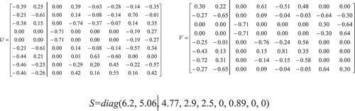
The main task of this phase is to project property terms and geographic features onto a reduced vector space using LSA technique. The Frobenius norm is adopted to determine the most significant k singular values to project property terms and geographic features onto the reduced k-dimensional vector space. Figure 2 shows the three constructed matrices, U, S and V, by performing SVD on the matrix in Table 1. According to the Frobenius norm, the value of k is calculated as 2 (for demonstration purposes, a threshold p = 0.8 is used). Therefore, the nine-dimensional vector space is reduced to a two-dimensional space.

Figure 2. An example: the produced three matrices, U, S and V, by SVD with dimension reduction (k = 2).

4.4. Categorizing geographic features

The main task in this phase is to assign geographic features to a set of predefined categories based on the reduced vector space generated from the previous phase. Similar to most studies in LSA-based information retrieval, this process is done by computing the similarity between geographic features against predefined categories. For that purpose, each category is represented as a query through a set of terms. These terms are specified with the support of ontologies, as detailed later in Section 5.

In LSA, a query can be treated just as another document because the query contains one or more terms. Given a query vector and a geographic feature vector, the similarity between them can be calculated by the cosine of the angle between these two vectors. In this way, the similarity values between the query and all geographic features can be obtained. More specifically, if the similarity value is greater than e, a similarity threshold, the geographic feature is considered to have a high similarity to the query. All these geographic features are assigned to the corresponding category. A geographic feature may be allocated to more than one category if the feature has high similarities to more than one query. Thus, overlapping group of geographic features, which is common in geographic feature categorization, can be obtained. For our example, assume that the term ‘Douglas fir’ is used to represent a query. The query vector, q, is then calculated as:

Subsequently, the cosine similarity between the vector query q and the vector d₁(for the geographic feature g₁) is calculated as:

Similarly, the cosine similarities between the query and the remaining seven geographic features are −0.2696, −0.1991, −0.6164, 0.7792, 0.9301, 0.9678 and −0.2696, respectively. Assuming the similarity threshold, e, is set as 0.85, three geographic features (g1, g6 and g7) are allocated to the same category that is associated with the property term ‘Douglas fir’. Although the geographic feature g6 does not contain the term ‘Douglas fir’ (Table 1), this feature is still selected. This is perhaps because the three property terms (namely, pinyon juniper, oak and ponderosa pine) in g6 also appear in g7. The results show that the LSA approach can capture not only the first-order co-occurrence (namely, two terms are co-occurring in one document) but also the second-order co-occurrence (namely, two terms not co-occurring in any of the documents while co-occurring with a third term).

Likewise, if the term ‘alligator juniper’ is used to represent a query, the cosine similarities between the query and the eight geographic features are −0.9824, −0.054, 0.0185, −0.4306, 0.8968, 0.9877, 0.9994 and −0.0540, respectively. Consequently, four geographic features (g1, g5, g6 and g7) are assigned to the same category associated with the term ‘alligator juniper’. Therefore, all three geographic features (g1, g6 and g7) are assigned to two different categories. In this way, overlapping categories are generated.

4.5. Assigning key concepts to geographic features

The cosine similarities, which were used earlier to categorize geographic features, are also used here to assign key words or key concepts to each generated category. In this context, each property term is treated as a query and the similarity values between the term and all geographic features that fall within the same category are calculated. The sum of all similarity values is then calculated to get the total similarity score for each term. After that, the scores for all property terms are normalized by dividing by the total number of property terms. The terms with scores greater than a predefined threshold, p_2, are selected as the key concepts to represent this category.

In our example, assuming that all of the eight geographic features fall in one category, the total similarities for each of the nine property terms to these features are calculated as 2.3219, 3.6908, 3.3460, 3.4112, 3.2033, 3.6908, 3.0051, 5.4487 and 2.6393, respectively. The normalization values are 0.26, 0.41, 0.37, 0.38, 0.36, 0.41, 0.33, 0.61 and 0.29, respectively. If threshold p₂ = 0.6 is used for key concepts, the property term ‘pinyon juniper’ is the only term that satisfies this threshold. Therefore, this term is selected as the key concept to represent the category that contains all the eight geographic features.

5. Empirical evaluation

In order to examine the effectiveness of the proposed method, an experiment was conducted to categorize a collection of text documents that describe mountains into categorizations. In the experiment, we chose mountains in the state of New Mexico in the United States. New Mexico is a mountainous state with diverse mountain groups that span an enormous range of geography and ecology.

5.1. Evaluation method

To evaluate the proposed method, a set of generated categories was evaluated against a set of predefined categories using precision, recall and F₁ score. These three measurements are widely used in information retrieval (Salton 1989). Precision (P) is the proportion of received instances that are relevant, while recall (R) is the proportion of relevant instances that are received. The F₁ score, the harmonic mean of the precision and recall, takes into account both P and R measures due to the trade-off between them. This is because greater precision decreases recall and greater recall leads to decreased precision. For a category i, these three measurements are defined as follows:

(1)

(2)

(3)

where TP_i is the number of mountains in both predefined and generated category i, FP_i is the number of mountains included in the generated but not in the predefined category i and FNi is the number of mountains included in the predefined category but not in the generated category i.

5.2. Experiment set-up

The state of New Mexico has more than 100 named mountains. We based on the following two sources to locate a mountain in New Mexico: (1) the book titled ‘The Mountains of New Mexico’ (Julyan 2006) and (2) Geographic Names Information System (GNIS) developed by the US Geological Survey (USGS). The first source provides comprehensive information for each mountain in New Mexico on several topics, including location, physiographic province, elevation, ecosystems, dimension, etc. This book, however, does not provide geographic coordinates of each mountain (e.g. altitude/longitude). Information on geographic coordinates is needed to generate a set of predefined categories, as detailed later. For that purpose, the second source, USGS GNIS, is used to obtain the geographic coordinates of mountains at the centre location. The data of USGS GNIS were downloaded from the New Mexico Resource Geographic Information System (NMRGIS, http://rgis.unm.edu/). All mountains that appeared in both Julyan (2006) and GNIS were selected, and they formed the set of geographic features (hereafter referred to as mountains) in the experiment.

The text that describes these mountains in New Mexico was also collected from Julyan (2006). Instead of considering all topics provided in the book, we only extracted terms related to ecosystems due to three reasons: (1) only one topic is selected in order to effectively analyse the association patterns between mountains and terms, (2) the ecosystem information for the majority of mountains in New Mexico (i.e. over 95% of mountains) is available in Julyan (2006) and (3) ecosystems are highly related to vegetation, a main property of mountains. Vegetation and associated major plants in the state of New Mexico are well studied in Dick-Peddie (1992).

A set of predefined categories along with the mountains belonging to each category is needed in order to calculate the three evaluation measurements (namely, precision, recall and F₁). To our knowledge, this kind of information is not available. Therefore, we generated this set based on the associated vegetation information of mountains in order to be consistent with the collected text. If two mountains fell within the same vegetation community type, these two mountains were considered under the same category. With this regard, we first downloaded a general vegetation map of New Mexico (in a .shp file) from NMRGIS. This map contained vector data for vegetation in New Mexico at a 1:1,000,000 scale, resulting in 16 vegetation community types. Second, we generated a buffer zone for each mountain due to the fact that the locations (altitude/longitude) of the mountains provided in GNIS are the centre locations, while mountains cover certain areas. The buffer zone for a mountain is determined based on the boundaries of individual mountains provided in Julyan (2006). Most commonly, the boundaries of individual mountains and mountain ranges are obvious, but not always. In Julyan (2006), the author estimated mountain boundary relying on his best judgment. After that, we generated a map layer for each vegetation community type. Based on these layers, mountains belonging to each type were obtained. In total, there are five vegetation community types that contain more than 10 mountains. These five types are montane coniferous forest, coniferous and mixed woodland, desert grassland, Chihuahuan Desert scrub and subalpine coniferous forest. These five vegetation community types were considered as the main types associated with the mountains in New Mexico, and they formed the set of predefined categories. Each mountain was then assigned to a predefined category if the mountain is within the corresponding vegetation community type layer. Table 2 lists the number of mountains in each predefined category. There are overlapping categories because a mountain might be within more than one vegetation community type map layer. Out of the 99 mountains, 19 mountains were only associated with one predefined category, 63 mountains were associated with two predefined categories and 9 mountains were associated with three predefined categories. There were no mountains associated with four or five predefined categories. The centre coordinates of these mountains and all 16 vegetation community types in the state of New Mexico are displayed in Figure 3.

Table 2. The predefined categories generated based on vegetation community types in the state of New Mexico.

Predefined categories	Number of mountains in categories
Montane coniferous forest	42
Coniferous and mixed woodland	45
Desert grassland	43
Chihuahuan Desert scrub	26
Subalpine coniferous forest	19

Figure 3. Mountains’ locations and vegetation community types in the state of New Mexico. Each point represents the centre location of a mountain.

As stated in Section 4, both extraction of property terms from text documents and determination of query terms for predefined categories are based on ontologies. For that purpose, two ontologies are needed in the experiment. One is a plant ontology and the other is a vegetation-type ontology. The plant ontology served as a controlled vocabulary to extract property terms, while the vegetation-type ontology was used to determine query terms. We followed the book ‘New Mexico Vegetation’ (Dick-Peddie 1992) to implement these two ontologies using Protégé (Noy, Fergerson, and Musen 2000), a widely used ontology development software program by Medical Informatics of Stanford University. This book provides categories of plants vegetation community types in New Mexico. This book also provides a comprehensive study of New Mexico’s vegetation and includes a detailed account of plant distribution information in the state. Moreover, vegetation community types used in Dick-Peddie (1992) are consistent with the downloaded vegetation map from NMRGIS.

The plant ontology contained common plants comprising vegetation in New Mexico, including four classes (trees, grasses, shrubs and forbs) and four relationships (has_common_name, has_scientific_name, has_definition and has_alternative_common_name). In addition, this ontology contained 384 instances, including 29 trees, 68 grasses, 114 shrubs and 173 forbs. Only terms that appeared in the common name or the alternative common name of these 384 instances were extracted from the collected documents to construct the ‘property term–geographic feature’ matrix for the further LSA process.

The vegetation-type ontology contained a hierarchy of classes, where each class represented a vegetation type in New Mexico and a subtype of a vegetation type was a subclass of the corresponding class. Each class/subclass might have the following six relationships: has_Dominant_Vegetation, has_CoDominant_Vegetation, has_Major_Trees, has_Major_Grasses, has_Major_Shrubs and has_Major_Forbs. The values of these six relationships were chosen based on the instances of the classes in the plant ontology. Therefore, the vegetation-type ontology was built upon the plant ontology. For example, subalpine coniferous forest is a class in the vegetation-type ontology. The value of its relationship ‘has_Dominant_Vegetation’ was assigned as Engelmann spruce, where Engelmann spruce is an instance of the class ‘tree’ in the plant ontology.

The query terms for each predefined category were obtained from the vegetation-type ontology. More specifically, the value of the relationship ‘has_Dominant_Vegetation’ of a vegetation type was chosen as the query term as this relationship presents the major plants comprising each type of vegetation type. As a result, the terms used to represent the five categories (subalpine coniferous forest, montane coniferous forest, coniferous and mixed woodland, desert grassland and Chihuahuan Desert scrub) are ‘Engelmann spruce’, ‘mixed coniferous forest’, ‘pinyon juniper’, ‘desert grasses’ and ‘Chihuahuan Desert scrub’, respectively.

To capture majority of ecosystem terms, all terms that appeared in at least two mountains but in less than 95% of all mountains were kept. In other words, given 100 mountains, if the term only appeared in one mountain, or the term appeared in over 95 documents, the term was removed. After removing these terms and the stop words, a total of 65 ecosystem terms remained and served as property terms in the LSA process. The TF-IDF value was calculated for each term in each mountain. These weights were the cell values in the ‘property term–geographic feature’ matrix. Following the steps stated in Section 4, the matrix was constructed and SVD and dimension reduction were then conducted on the matrix in MATLAB to project the ecosystem terms and mountains onto a reduced vector space, respectively. After that, a set of generated categories were obtained and key concepts were assigned to each category as discussed in Section 4.

5.3. Experiment results and discussion

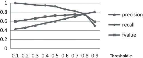
As described in Section 4, the categorization results depend on two main parameters: threshold p (to determine the reduced dimension of the vector space) and threshold e (to determine the similar geographic features). A total of 200 categorizations were conducted based on all combinations of p and e, where p is from 0.5 to 0.9 and e is from 0.1 to 0.9. Both are in increments of 0.05. Figure 4 shows the F₁ score with the combinations of p and e. The best categorizing result was found with F₁ = 0.7465 when threshold p was 0.6 and threshold e was 0.8. Therefore, we applied such values of p and e to the further analysis.

Figure 4. F₁ scores and threshold p.

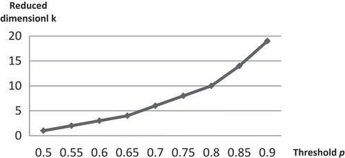
The dimension of the vector space dropped with the decrease of the threshold p. As shown in Figure 5, when p was 0.6, the dimension of the vector space reduced to 3 from the original 63, with a reduction rate of 95%. Each ecosystem term in the 63 words represents a dimension in the original vector space. By examining these 63 terms, synonymy is quite common, such as pinyon juniper and pinyon juniper forest, spruce and spruce fir, etc., although no polysemy was found in these 63 terms. By using SVD on the ‘property term–geographic feature’ matrix with the TF-IDF values and then applying the Frobenius norm, the best result was attained by reducing the transformed vector space from 63 to 3. In other words, this three-dimensional vector space can represent the contextual-usage meaning of these 63 ecosystem terms well, including those semantic similar terms.

Figure 5. Reduced dimension k and threshold p.

Precision increased while the recall decreased with the increase of the threshold e. Figure 6 shows the precision, recall and F₁ score for various e values when the threshold p was 0.6. When threshold e was 0.1, the precision value was 0.42, but the recall value reached 1, while when threshold e was increased to 0.9, the precision value increased to 0.81, but the recall value dropped to 0.50. F₁ score, the trade-off between precision and recall, slowly increased with the increase of threshold e and reached the highest value when threshold e was 0.8. After that, the value dropped quickly with the increase of threshold e. The results demonstrate an inverse relationship between precision and recall. Based on the theory of precision and recall, the recall value could be increased by classifying more correct mountains, but this increase would come at the cost of increasing the number of irrelevant mountains (namely, decreasing precision). These experiments also show that usually a lower threshold e should be chosen if we hope to allocate as many mountains as possible in the predefined category to the corresponding generated category (namely, high recall value). In contrast, a higher threshold e should be chosen if we hope that the majority of allocated mountains in the generated category are actually in the predefined category (namely, high precision value).

Figure 6. Precision, recall and F₁ score values with threshold e (p = 0.6).

Table 3 shows the confusion matrix of the categorization experiment when threshold p is 0.6 and threshold e is 0.8. As mentioned above, these values reached the best F₁ score with 0.7465. For example, for the category ‘coniferous and mixed woodland’, 40 out of 99 mountains are not in either a predefined or a generated category (true negatives, TN), 32 mountains are in both predefined and generated category (true positives, TP), 14 mountains are in generated but not in predefined category (false positives, FP) and 13 mountains are in predefined but not in generated category (false negatives, FN). Among these five categories, the category ‘subalpine coniferous forest’ has the highest precision value with 1.0, while its recall value is quite low (0.6842). The category ‘Chihuahuan Desert scrub’ has the highest recall value with 0.9231, while its precision value is quite low (0.6316). This matrix also shows an inverse relationship between precision and recall, that is, a high recall value is often associated with a low precision value, while a high precision value is often associated with a low recall value.

Table 3. The categorization results (p = 0.6, e = 0.8).

Vegetation category	TN	TP	FP	FN	Precision	Recall	F1 score
Coniferous forest	48	27	9	15	0.7500	0.6429	0.6923
Coniferous and mixed woodland	40	32	14	13	0.6957	0.7111	0.7033
Desert grassland	42	36	14	7	0.7200	0.8372	0.7742
Chihuahuan Desert scrub	59	24	14	2	0.6316	0.9231	0.7500
Subalpine coniferous forest	80	13	0	6	1.0000	0.6842	0.8125
			Overall F1 score: 0.7465

TN (true negatives): not in each generated or predefined category; TP (true positives): in both generated and predefined category; FP (false positives): in generated but not in predefined category; FN (false negatives): in predefined but not in generated category.

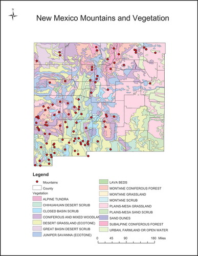
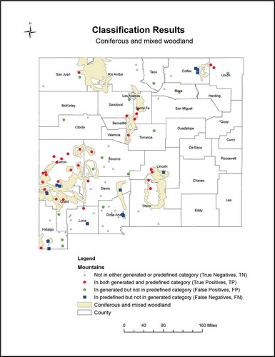
In order to visually see the locations of those correctly or incorrectly allocated mountains, Figure 7 shows a map of the categorization results for the predefined and generated category ‘coniferous and mixed woodland’, the largest group in the predefined category (45 mountains). Results showed that 46 mountains were allocated to the corresponding generated category. Of these 46 mountains, 32 mountains (in the red circle) were also in the predefined category, while 14 mountains (in the green pentagon) were not. In other words, 32 out of 45 mountains in the predefined category were correctly grouped to a generated category, while 13 were not (in the blue square). By examining the locations and descriptions of mountains that were not correctly allocated to a corresponding category, their ecosystem descriptions and the associated vegetation types were not consistent. For example, the ecosystem description of mountain ‘Florida Mountains’, which is located in Luna County, is ‘evergreen oak, junipers, beargrass, mesquite, ocotillo, cacti, yucca’. In the predefined category, based on the spatial relationship between vegetation types and the location, this mountain was assigned to three categories: ‘woodland’, ‘Chihuahuan Desert grassland’ and ‘Chihuahuan Desert scrub.’ However, based on the description, this mountain was only allocated to two categories, ‘Chihuahuan Desert grassland’ and ‘Chihuahuan Desert scrub’, but not to ‘coniferous and mixed woodland’.

Figure 7. Categorization results: a map of mountains for the predefined and generated category ‘coniferous and mixed woodland’ (p = 0.6, e = 0.8).

As for the overlapping categories, a total of 65 mountains were allocated to two generated categories. Of these 65 mountains, 45 were exactly matched to the corresponding predefined overlapping categories. As mentioned earlier, 63 mountains were allocated to two predefined categories. Similar to the predefined categories, there were no mountains assigned to four or five categories. Seven mountains were allocated to three generated categories, but none of them matched the nine mountains that were assigned to three predefined categories. The results show that this approach is effective in dealing with the majority overlapping categories (namely, assigning a mountain to two categories) and the less common overlapping categories (namely, assigning a mountain to four or five categories). In this experiment, the approach is difficult in dealing with mountains that fell into three categories. The main reason could be the completeness of the terms of ecosystems used to describe mountains in the documents collected from Julyan (2006). Allocating a mountain to one or more categories heavily depends on these terms, but only main terms for each mountain are provided in Julyan (2006).

The key concepts used to represent each generated category using the value of threshold (p₂) 0.8 are listed in Appendix A. The numbers of key concepts for the five categories were 4, 5, 14, 20 and 10, respectively. Three categories (1, 2 and 5) generated a reasonable size of key concepts; however, categories 3 and 4 generated too many key concepts. Examining the ecosystem terms of the mountains in these two categories showed that most of these words appeared in each mountain. As for the generated key concepts, the query term used for each category was identified in the corresponding category. In addition, more key concepts were identified for each category. For example, besides the query term ‘mixed conifer’, three more words (‘Douglas fir’, ‘ponderosa pine’ and ‘spruce fir’) were identified as key concepts for the category ‘coniferous forest’. By examining the vegetation-type ontology, the term ‘Douglas fir’ is the co-dominant vegetation (namely, the relationship has_coDominant_Vegetation) of the coniferous forest. The other two concepts are among the major trees of the coniferous forest. The results showed that the proposed approach based on LSA and ontology can capture the main concepts that represent the categories.

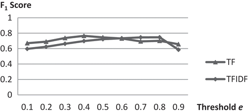
Although TF-IDF is generally a better way than TF to construct the ‘property term–geographic feature’ matrix, this experiment also investigated the TF method. Results showed that for this data set, both TF and TF-IDF provided good results; TF reached a higher F₁ score with 0.7465 but with different parameters (p = 0.65, e = 0.9). This is perhaps because most of the terms only appear once in one document. Figure 8 shows a comparison of TF and TF-IDF at different threshold e when p = 0.7, where both TF and TF-IDF had the same reduced dimension (k = 3). However, using TF methods, the numbers of key concepts for the five categories were 29, 25, 30, 30 and 25, respectively (see Appendix A). This method is not effective in capturing key concepts to present generated categories because too many key concepts were included in each category.

Figure 8. Comparison of TF and TF-IDF with threshold e.

6. Conclusion and future work

This paper proposed a method to conceptually categorize geographic features from text based on LSA and ontologies. The experimental results indicate that the proposed method achieves satisfactory categorization effectiveness through capturing and extracting the semantic context of terms. The results also show that this method can efficiently deal with synonymy in the description of geographic features and can extract key concepts to represent categories. The type of a geographic feature, together with its name and footprint (e.g. latitude and longitude coordinates), is the core element for each feature in a gazetteer (Hill 2000), which in turn serves as a foundation for a wide variety of tools and applications, including geographic information mining and digital library (Larson 1996). Name and footprint of a geographic feature are usually well defined, and methods for extracting them from the text have been well developed (Goldberg, Wilson, and Knoblock 2009). Our method will be valuable for geographic feature categorization by providing a way to automatically assign a geographic feature to one or more categories from text, particularly the documents that contain many domain-specific terminologies.

The proposed method is driven by ontologies. In addition to using concepts in the ontologies to serve as a set of controlled terms, the relationships between these concepts specified in the ontologies are also used to incorporate domain knowledge in the process of categorizing geographic features from text. The method presented in this paper is expected to advance research in ontologies of geographic information. The experiments can be extended to categorizing other geographic features from text with the support of the appropriate domain ontologies.

Several limitations arise from this research. As reported, this method needs to select the appropriate corpus of texts. Similar to any corpus-based approach, this method relies on the collected text that describes geographic information. It is desirable to have a collection of text that provides accurate and complete description of geographic features. When the quality of the text is low or when the text cannot be trusted to be a representative of geographic features, the categorization results could not be trusted completely. In the literature, many efforts have been made to evaluate the quality of text for the performance of LSA (Kontostathis and Pottenger 2006). Although each application is different, common wisdom holds that the corpus should consist of texts that are relevant to the particular domain task (Wiemer-Hastings 1999). This is because a domain-specific corpus will usually have higher relevant words and will thus not waste its representational power on words that will not be seen by the applications.

Second, the performance of the proposed method depends on the ontologies. The method uses ontologies to control the terms extracted from the collected text and to determine the query terms to represent the predefined categories. The ontologies should be relevant to the collection and the concepts and their relationships present in the collections should be thoroughly represented in the ontology, otherwise this method might have a poor performance. In this experiment, we generated ontologies from a comprehensive study of mountains and vegetation types in New Mexico. The ontologies should be specified when this method is applied to other applications. Another limitation of the research is the scope of the evaluation. This paper mainly focuses on valuation and discussion of the two parameters involved in the method for one type of geographic feature data set. This provides new insight into the evaluation and analysis of the proposed method. One goal of future research is to apply the method to the description of other types of geographic features and to examine categorization accuracy and overlapping class rate.

The current research focuses on classifying geographic features into a set of predefined categories. Another opportunity for future research is to extend this method to a set of previously unseen categories. Query terms could be obtained from directly grouping terms, a main application of LSA, instead of using values from the relationships in ontologies. Furthermore, some other state-of-the-art topic models, such as latent Dirichlet allocation (Blei, Ng, and Jordan 2003), could be explored to categorize geographic features from text in the future.

Acknowledgements

The author would like to thank anonymous reviewers for their valuable comments and suggestions.

Disclosure statement

No potential conflict of interest was reported by the author.

Appendix A. Comparison of the TF-IDF and TF in terms of key concept identification (p₂ = 0.8).

Category	Number of terms	Key concepts
TF-IDF method
Coniferous forest	4	Douglas fir (0.83), mixed conifer (0.86), ponderosa pine (0.81), spruce fir (0.86)
Coniferous and mixed woodland	7	Alligator juniper (0.83), fir (0.80), grasses (0.84), pinyon juniper (0.86), pinyon pine (0.88), ponderosa pine (0.82), spruce (0.81)
Desert grassland	14	Chihuahuan Desert grasses (0.80), Chihuahuan Desert scrub (0.84), Chihuahuan Desert shrubs (0.82), evergreen oak (0.81), lower Sonoran grasses (0.81), lower Sonoran shrubs (0.81), agave (0.87), desert grasses (0.80), live oak (0.85), ocotillo (0.82), pinyon (0.80), saltbush (0.83), shrubs (0.86), yucca (0.84)
Chihuahuan Desert scrub	20	Chihuahuan Desert grasses (0.88), Chihuahuan Desert scrub (0.91), Chihuahuan Desert shrubs (0.90), evergreen oak (0.90), lower Sonoran grasses (0.90), lower Sonoran shrubs (0.90), manzanita (0.83), agave (0.92), bluestem (0.84), creosote bush (0.82), desert grasses (0.90), grama grasses (0.89), junipers (0.80), live oak (0.92), mesquite (0.85), ocotillo (0.90), pinyon (0.84), saltbush (0.91), shrubs (0.93), yucca (0.92)
Subalpine coniferous forest	10	Douglas fir (0.98), Engelmann spruce (0.95), Great Basin grassland (0.90), alpine grasses (0.92), alpine sedges (0.92), aspen (0.96), blue spruce (0.96), mixed conifer (0.87), subalpine fir (0.93), white fir (0.93)
TF method
Coniferous forest	29	Arizona white oak (0.91), Douglas fir (0.92), Engelmann spruce (0.86), Gambel oak (0.81), Great Basin grassland (0.86), Indian rice grass (0.86), upper Sonoran desert grasses (0.96), upper Sonoran desert shrubs (0.96), alpine grasses (0.85), alpine sedges (0.85), Apache plume (0.97), aspen (0.90), blue spruce (0.87), chamisa (0.95), cholla (0.97), fir (0.92), galleta (0.86), grasses (0.89), grey oak (0.86), mid-grass prairie (0.98), mixed conifer (0.98), pinyon juniper (0.98), pinyon pine (0.95), ponderosa pine (0.96), short-grass steppe (0.98), spruce (0.94), spruce fir (0.96), subalpine fir (0.86), white fir (0.90)
Coniferous and mixed woodland	25	Arizona white oak (0.90), Douglas fir (0.86), Engelmann spruce (0.80), Gambel oak (0.83), Indian rice grass (0.87), upper Sonoran desert grasses (0.94), upper Sonoran desert shrubs (0.94), Apache plume (0.95), aspen (0.84), blue spruce (0.80), chamisa (0.93), cholla (0.95), fir (0.87), galleta (0.87), grasses (0.89), grey oak (0.87), mid-grass prairie (0.94), mixed conifer (0.95), pinyon juniper (0.94), pinyon pine (0.93), ponderosa pine (0.92), short-grass steppe (0.94), spruce (0.89), spruce fir (0.94), white fir (0.84)
Desert grassland	30	Chihuahuan Desert grasses (0.95), Chihuahuan Desert grasslands (0.91), Chihuahuan Desert scrub (0.93), Chihuahuan Desert shrubs (0.95), Chihuahuan pine (0.94), Emory oak (0.87), evergreen oak (0.92), lower Sonoran grasses (0.95), lower Sonoran shrubs (0.95), manzanita (0.93), agave (0.96), beargrass (0.89), cacti (0.96), creosote bush (0.93), desert grasses (0.93), grama (0.96), grama grasses (0.93), junipers (0.92), live oak (0.96), mesquite (0.94), mountain mahogany (0.94), ocotillo (0.95), pinyon (0.96), prickly pear (0.87), saltbush (0.94), semi-desert grassland (0.84), shrubs (0.96), stool (0.96), tarbush (0.92), yucca (0.95)
Chihuahuan Desert scrub	30	Chihuahuan Desert grasses (0.99), Chihuahuan Desert grasslands (0.98), Chihuahuan Desert scrub (0.99), Chihuahuan Desert shrubs (1.00), Chihuahuan pine (0.94), Emory oak (0.84), evergreen oak (0.98), lower Sonoran grasses (0.99), lower Sonoran shrubs (0.99), manzanita (0.98), agave (0.99), beargrass (0.87), cacti (0.99), creosote bush (0.99), desert grasses (0.99), grama (0.99), grama grasses (0.98), junipers (0.98), live oak (1.00), mesquite (0.99), mountain mahogany (0.94), ocotillo (0.99), pinyon (0.99), prickly pear (0.84), saltbush (0.99), semi-desert grassland (0.80), shrubs (0.98), stool (0.99), tarbush (0.98), yucca (0.99)
Subalpine coniferous forest	25	Arizona white oak (0.85), Douglas fir (0.98), Engelmann spruce (0.95), Great Basin grassland (0.94), upper Sonoran Desert grasses (0.94), upper Sonoran Desert shrubs (0.94), alpine grasses (0.94), alpine sedges (0.94), apache plume (0.96), aspen (0.97), blue spruce (0.95), chamisa (0.91), cholla (0.96), fir (0.98), grasses (0.83), mid-grass prairie (0.99), mixed conifer (0.97), pinyon juniper (0.98), pinyon pine (0.91), ponderosa pine (1.00), short-grass steppe (0.98), spruce (0.99), spruce fir (0.93), subalpine fir (0.94), white fir (0.97)

References

- Baharudin, B., L. Lee, and K. Khan. 2010. “A Review of Machine Learning Algorithms for Text-Documents Classification.” Journal of Advances in Information Technology 1 (1): 4–20. doi:10.4304/jait.1.1.4-20.
- Bian, L., and S. Hu. 2007. “Identifying Components for Interoperable Process Models Using Concept Lattice and Semantic Reference System.” International Journal of Geographical Information Science 21 (9): 1009–1032. doi:10.1080/13658810601169907.
- Blei, D., A. Ng, and M. Jordan. 2003. “Latent Dirichlet Allocation.” Journal of Machine Learning Research 3: 993–1022.
- Chen, R., J. Liang, and R. Pan. 2008. “Using Recursive ART Network to Construction Domain Ontology Based on Term Frequency and Inverse Document Frequency.” Expert Systems with Applications 34: 488–501. doi:10.1016/j.eswa.2006.09.019.
- Comber, A., A. Lear, and R. Wadsworth. 2010. “A Comparision of Different Semantic Methods for Integrating Thematic Geographical Information: The Example of Land Cover.” 13th AGILE International Conference on Geographic Information Science, Guimaraes, May 10–14. Edited by J. Carswell and T. Tekuza.
- Deerwester, S., S. Dumais, G. Furnas, T. Landauer, and R. Harshman. 1990. “Indexing by Latent Semantic Analysis.” Journal of the American Society for Information Science 41 (6): 391–407. doi:10.1002/(ISSN)1097-4571.
- Denhiere, G., B. Lemaire, C. Bellissens, and S. Jhean-Larose. 2006. “A Semantic Space for Modeling Children’s Semantic Memory.” In Handbook of Latent Semantic Analysis, edited by T. K. Landauer, D. S. McNamara, S. Dennis, and W. Kintsch, 143–165. Mahwah, NJ: Lawrence Erlbaum Associates, Publishers.
- Dick-Peddie, W. 1992. New Mexico Vegetation: Past, Present, and Future. Albuquerque: University Of New Mexico Press.
- Duckham, M., and M. Worboys. 2005. “An Algebraic Approach to Automated Geospatial Information Fusion.” International Journal of Geographical Information Science 19 (5): 537–557. doi:10.1080/13658810500032339.
- Fabrikant, S., D. Montello, M. Ruocco, and R. Middleton. 2004. “The Distance-Similarity Metaphor in Network-Display Spatializations.” Cartography and Geographic Information Science 31 (4): 237–252. doi:10.1559/1523040042742402.
- Fisher, D. 1987. “Knowledge Acquisition via Incremental Conceptual Clustering.” Machine Learning 2: 139–172. doi:10.1007/BF00114265.
- Goldberg, D., J. Wilson, and C. Knoblock. 2009. “Extracting Geographic Features from the Internet to Automatically Build Detailed Regional Gazetteers.” International Journal of Geographical Information Science 23 (1): 93–128. doi:10.1080/13658810802577262.
- Gruber, T. 1993. “A Translation Approach to Portable Ontology Specifications.” Knowledge Acquisition 5 (2): 199–220. doi:10.1006/knac.1993.1008.
- Guarino, N. “Formal Ontology and Information System.” 1998. In Formal Ontology in Information Systems. Proceedings of FOIS’98, Trento, Italy June, edited by N. Guarino, 3–15. Amsterdam: IOS Press.
- Hearst, M. 1999. “The Use of Categories and Clusters for Organizing Retrieval Results.” In Natural Language Information Retrieval, edited by T. Strzalkowski, 333–374. Dordrecht, The Netherland: Kluwer Academic.
- Hill, L. L. 2000. “Core Elements of Digital Gazetteers: Placenames, Categories, and Footprints.” In Proceedings of Research and Advanced Technology for Digital Libraries, 4th European Conference (ECDL ‘00), edited by J. L. Borbinha, and T. Baker, 280–290. Vol. 1923. London: Springer.
- Huang, Y. 2011. “A Latent Semantic Analysis-Based Approach to Geographic Feature Categorization from Text.” In Proceedings of the Fifth IEEE International Conference on Semantic Computing, edited by S. Guadarrama and N. Ludwig. Palo Alto, CA: Stanford University.
- Julyan, R. 2006. The Mountains of New Mexico. Albuquerque: University of New Mexico Press.
- Kavouras, M., and M. Kokla. 2002. “A Method for the Formalization and Integration of Geographical Categorizations.” International Journal of Geographical Information Science 16 (5): 439–453. doi:10.1080/13658810210129120.
- Kobayashi, M., and M. Aono. 2006. “Exploring Overlapping Clusters Using Dynamic Re-Scaling and Sampling.” Knowledge Information Systems 10 (3): 295–313. doi:10.1007/s10115-006-0005-y.
- Kontostathis, A., and W. Pottenger. 2006. “A Framework for Understanding Latent Semantic Indexing (LSI) Performance.” Information Processing & Management 42: 56–73. doi:10.1016/j.ipm.2004.11.007.
- Kuhn, W. 2002. “Modelling the Semantics of Geographic Categories through Conceptual Integration.” In Proceedings of the Second International Conference on Geographic Information Science – GIScience, edited by M. Egenhofer and D. Mark, 108–118. London: Springer-Verlag.
- Kumar, M. A., and M. Gopal. 2010. “A Comparison Study on Multiple Binary-Class SVM Methods for Unilabel Text Categorization.” Pattern Recognition Letters 31 (11): 1437–1444. doi:10.1016/j.patrec.2010.02.015.
- Landauer, T., and S. Dumais. 1997. “A Solution to Plato’s Problem: The Latent Semantic Analysis Theory of Acquisition, Induction, and Representation of Knowledge.” Psychological Review 104 (2): 211–240. doi:10.1037/0033-295X.104.2.211.
- Landauer, T., P. Foltz, and D. Laham. 1998. “An Introduction to Latent Semantic Analysis.” Discourse Processes 25 (2–3): 259–284. doi:10.1080/01638539809545028.
- Larson, R. 1996. “Geographic Information Retrieval and Spatial Browsing.” In Geographic Information Systems and Libraries: Patrons, Maps, and Spatial Information, edited by L. C. Smith and M. Gluck, 81–124. Champaign: University of Illinois at Urbana–Champaign.
- Lieberman, M. S., H. Samet, J. Sankaranarayanna, and G. J. Sperlin. 2007. “STEWARD: Arthitecture of a Spatio-Textual Search Engine.” In Proceedings of the 15th ACM Int. Symp. on Advances in GIS (ACMGIS’07), edited by H. Samet, C. Shahabi, and M. Schneider, 186–193. New York: ACM.
- Mark, D., B. Smith, and B. Tversky. 1999. “Ontology and Geographic Objects: An Empirical Study of Cognitive Categorization.” COSIT’99, LNCS 1661, Stade, August 25–29, 283–298. Edited by C. Freksa and D. M. Mark.
- Michalski, R. S. 1980. “Knowledge Acquisition through Conceptual Clustering: A Theoretical Framework and an Algorithm for Partitioning Data into Conjunctive Concepts.” Journal of Policy Analysis and Information Systems 4 (3): 219–244.
- Millis, K., J. Magliano, K. Wiemer-Hastings, S. Todaro, and D. MxNamara. 2006. “Assessing and Improving Comprehension with Latent Semantic Analysis.” In Handbook of Latent Semantic Analysis, edited by T. K. Landauer, D. S. McNamara, S. Dennis, and W. Kintsch, 207–225. Mahwah, NJ: Lawrence Erlbaum Associates, Publishers.
- Noy, N. F., R. W. Fergerson, and M. A. Musen. 2000. “The Knowledge Model of Protégé 2000: Combining Interoperability and Flexibility.” Proceedings of the 12th International Conference on Knowledge Engineering and Knowledge Management (EKAW’2000), Juan-les-Pins, October 2–6. Edited by R. Dieng and O. Corby.
- Nunzio, G. 2009. “Using Scatterplots to Understand and Improve Probabilistic Models for Text Categorization and Retrieval.” International Journal of Approximate Reasoning 50 (7): 945–956. doi:10.1016/j.ijar.2009.01.002.
- Odgers, N., A. McBratney, and B. Minasny. 2011. “Bottom-Up Digital Soil Mapping. I. Soil Layer Classes.” Geoderma 163: 38–44. doi:10.1016/j.geoderma.2011.03.014.
- Rauch, E., M. Bukatin, and K. Baker. 2003. “A Confidence-Based Framework for Disambiguating Geographic Terms.” In Proceedings of the HLT-NAACL 2003 Workshop on Analysis of Geographic References, edited by S. Kornai and B. Sundheim, 50–54. Morristown, NJ: Association for Computational Linguistics.
- Robertson, S. 2004. “Understanding Inverse Document Frequency: On Theoretical Arguments for IDF.” Journal of Documentation 60 (5): 503–520. doi:10.1108/00220410410560582.
- Salton, G. 1989. Automatic Text Processing - The Transformation, Analysis, and Retrieval of Information by Computer. Reading, MA: Addison-Wesley.
- Sebastiani, F. 2002. “Machine Learning in Automated Text Categorization.” ACM Computing Surveys 34 (1): 1–47. doi:10.1145/505282.505283.
- Smith, B., and D. Mark. 2001. “Geographical Categories: An Ontological Investigation.” International Journal of Geographical Information Science 15 (7): 591–612. doi:10.1080/13658810110061199.
- Smith, B., and D. Mark. 2003. “Do Mountains Exist? Towards an Ontology of Landforms.” Environment and Planning B: Planning and Design 30 (3): 411–427. doi:10.1068/b12821.
- Song, W., and S. Park. 2009. “Genetic Algorithm for Text Clustering Using Ontology and Evaluating the Validity of Various Semantic Similarity Measures.” Expert Systems with Applications 36: 9095–9104. doi:10.1016/j.eswa.2008.12.046.
- Srinivasan, P. 2001. “Meshmap: A Text Mining Tool for Medline.” In Proc. AMIA Symp, edited by S. Bakken, November 3–7, 642–646. Washington, DC.
- Uguz, H. 2011. “A Two-Stage Feature Selection Method for Text Categorization by Using Information Gain, Principal Component Analysis and Genetic Algorithm.” Knowledge-based Systems 24 (7): 1024–1032. doi:10.1016/j.knosys.2011.04.014.
- Usery, L. 1993. “Category Theory and the Structure of Features in Geographic Information Systems.” Cartography and Geographic Information Science 20 (1): 5–12. doi:10.1559/152304093782616751.
- Wei, C., C. Yang, and C. Lin. 2008. “A Latent Semantic Indexing-Based Approach to Multilingual Document Clustering.” Decision Support Systems 45: 606–620. doi:10.1016/j.dss.2007.07.008.
- Wiemer-Hastings, P. 1999. “How Latent Is Latent Semantic Analysis?” In Proceedings of the Sixteenth International Joint Conference on Artificial Intelligence, edited by T. Dean, 932–937. San Francisco, CA: Morgan Kaufmann.
- Wise, J. A., J. J. Thomas, K. Pennock, D. Lantrip, M. Pottier, A. Schur, and V. Crow. 1995. “Visualizing the Non-Visual: Spatial Analysis and Interaction with Information from Text Documents.” In Information Visualization, 1995. Proceedings, edited by N. Gershon and S. Eick, Atlanta, October 30, 51–58. IEEE.
- Yu, B., Z. Xu, and C. Li. 2008. “Latent Semantic Analysis for Text Categorization Using Neural Network.” Knowledge-Based Systems 21: 900–904. doi:10.1016/j.knosys.2008.03.045.
- Zha, H., and H. Simon. 1998. “A Subspace-Based Model for Latent Semantic Indexing in Information Retrieval.” In Proceedings of the Thirteenth Symposium on the Interface, edited by W. Eddy, 315–320. New York: Springer-Verlag.
- Zheng, H., C. Borchert, and Y. Jiang. 2010. “A Knowledge-Driven Approach to Biomedical Document Conceptualization.” Artificial Intelligence in Medicine 49 (2): 67–78. doi:10.1016/j.artmed.2010.02.005.