Mapping sex offender activity spaces relative to crime using time-geographic methods

ABSTRACT

Activity spaces describe the physical area typically encountered by an individual person during his or her routine daily activities. Activity spaces encompass a person’s anchor points – locations that are frequented regularly, such as home, work, school, and recreational areas – and the travel paths that connect them. Activity spaces of criminals are routinely mapped in order to better understand the spatial patterns and processes of crime at the individual level. Although many geographic information system-based methods have been used to map activity spaces over the years, potential path areas are becoming a preferred method since they incorporate both spatial and temporal data, as well as time budget and mobility constraints. This paper extends potential path areas for mapping activity spaces of criminals in two ways. First, time-geographic density estimation (TGDE) is used to estimate individual activity spaces using potential path areas that have associated probability densities. Second, activity spaces of numerous individuals are combined into a single intensity surface that maps areas of a city that are more frequented by offenders and, accordingly, expected to support higher crime rates. The approach is demonstrated using a dataset of home and work addresses of registered sex offenders in the city of St. Louis. The final density surface of their combined activity spaces is related to the locations of reported sex crimes. The results highlight how sex crimes are concentrated in offender activity spaces and suggest the approach might be useful for predictive policing.

KEYWORDS:

• Time geography
• density estimation
• hot spots
• sex offenders

Criminologists and geographers alike have long been interested in analysing and understanding spatial patterns of crime (Bailey and Gatrell 1995). Individual crimes result from the intersection of three necessary conditions: a motivated offender desiring to commit a crime, identification of a suitable target by the offender, and the absence of a capable guardian that poses risk of detection, such as a law enforcement officer or other security measure (Cohen and Felson 1979; Sherman, Gartin, and Buerger 1989). In a spatial context, the journey-to-crime literature describes how the majority of crimes, especially violent ones, are committed in close proximity to locations the offender frequently visits for routine activities – termed anchor points – such as places of residence, work, school, or recreation (see Andresen, Frank, and Felson 2014, for a review). Crime pattern theory explains that an offender is most likely to commit crimes in the physical area encompassing these anchor points and the travel paths among them, collectively termed an activity space (Brantingham and Brantingham 1993). Most crimes are committed in an offender’s activity space, as that is the region with which he or she has the most familiarity with suitable targets and awareness of capable guardians (Ratcliffe 2006).

Mapping observed or predicted activity spaces can be extremely useful in policing as a means to prevent future crimes and as a tool to solve past ones. Activity spaces have been mapped and analysed using several approaches, not just for studying crime but for such diverse applications as measuring health-care accessibility (Sherman et al. 2005), mapping food environments (Kestens et al. 2010), and planning transit developments (Harding et al. 2012). In some cases, activity spaces are simply described qualitatively using a person’s self-reported activity locations (Mason and Korpela 2009). Activity spaces have been visualised using mental maps hand-drawn by individuals of interest (Paulsen, Bair, and Helms 2009). More commonly, geographic information system (GIS) is used to delineate the spatial extent of activity spaces. The earliest method was the standard deviational ellipse, a simple approximation of the region containing anchor points (Yuill 1971). Other studies have defined activity spaces by connecting anchor points with the shortest paths (Zenk et al. 2011) or by buffering those paths to encompass a wider spatial area (Martinez, Lorvick, and Kral 2014). Alternatively, activity spaces have been delineated by enclosing anchor points with a polygon, such as the ones created using minimum convex hulls (Villanueva et al. 2012). Kernel density methods (Silverman 1986), which create a smoothed intensity surface from a set of points, have also been used to map activity spaces (Kamruzzaman et al. 2011).

More recently, potential path areas, a concept derived from time geography, have been popular for mapping activity spaces (see Patterson and Farber 2015, for a review). Potential path areas delineate all locations that are accessible to an individual given the spatial locations and time stamps of anchor points, a specified time budget for activities, and mobility constraints. Ratcliffe (2006) was the first to use potential path areas to map activity spaces of criminals, followed by applications by Kuijpers, Grimson, and Othman (2011), Morgan and Steinberg (2013), and Downs (2014). The present paper extends the approach of mapping offender activity spaces using more advanced methods of time geography based on potential path areas or trees. First, time-geographic density estimation (TGDE) is used to create individual potential path areas that have associated probability densities that are reflective of spatial differences in familiarity and awareness. Second, the activity spaces of numerous offenders are combined into a single intensity surface that maps areas of a city that are more frequented by offenders and, accordingly, expected to support higher crime rates. The approach is demonstrated using a data set of home and work addresses of registered sex offenders in the city of St. Louis. The final density surface of their combined activity spaces is related to the locations of reported sex crimes. The results of the findings are used to guide a discussion of the approach’s applicability for other types of analyses.

Background

Time geography was first theorised by Torsten Hägerstrand (1970) as a way to understand how people’s potential movements through space and time are limited by various factors such as employment locations, personal mobility, and working hours. Although Hägerstrand’s work was largely conceptual at the outset, time geography has grown into a rigorous framework in geographic information science for studying the constrained movements of people and other objects (Miller 2005a). Given the known spatial and temporal information of an object’s whereabouts, methods of time geography can be used to delineate all of its possible locations at any time. Miller’s (2005b) work provides the underlying mathematical foundations for these computations using the basic elements of time geography: the space-time path, the space-time prism, and the potential path area.

All of these basic elements of time geography are derived from control points, which are known spatial locations of an object at particular times. Control points can be fixed anchor points for an individual, such as home and work addresses, or regularly captured tracking data such as those collected by GPS. In continuous geographic space, the space-time path is constructed by connecting consecutive control points with straight line segments; in network spaces, like road systems, it is represented as the shortest pathway along the network between those locations. Given some estimate of the object’s maximum velocity, the prism delineates all areas along the space-time path that were reachable by the object at any time. For any two consecutive control points, this area mapped in geographic space is termed the potential path area. In continuous space the potential path area takes the shape of an ellipse. In network space the potential path area shows all accessible areas along the network and forms what is termed a potential path tree. Figure 1 shows a generic space-time path, a space-time prism, and a potential path area in geographic space. These basic elements have proven useful for mapping the potential movements of people (Kwan 1999), vehicles (Kuijpers et al. 2010), and animals (Downs, Horner, and Tucker 2011).

Figure 1. A space-time path and prism for two consecutive points.

A recent advancement in geographic information science is the development of a statistical or probabilistic framework time geography. Rather than simply mapping the potential locations for objects, these methods quantify which locations are more probable. Two main approaches have been used. The first involves assigning probabilities to locations within the space-time prism at discrete time intervals (Winter and Yin 2010; Downs et al. 2014). This allows analysts to calculate the probability of finding a particular individual at any location at any time. The second, TGDE, creates a probability density surface of an object’s movements over its entire tracking interval (Downs 2010). The result is an intensity map that shows where the object could have spent the largest amount of time, or alternatively its most likely locations. The network formulation of TGDE (Downs and Horner 2012), which produces probabilistic potential path trees along street networks, is used in this paper.

Downs and Horner (2012) describe the network formulation of TGDE, which is useful for mapping peoples’ movements in cities (Horner and Downs 2014). In simple terms, the method generates potential path trees for each pair of control points in the data set, applies a distance weighting function to each tree to smooth the probability density, and combines all trees to create a cumulative intensity surface. It works in the exact same manner as traditional kernel density estimation (Silverman 1986), except a distance-weighting function of the potential path tree for each pair of points is used instead of a two-dimensional kernel function applied to each single point. Network-based TGDE can be calculated using Equation (1) as

(1)

where:

the density estimate at any location x on a network,

= the number of control points in a data set, where consecutive points are denoted and ,

= distance weighting function of potential path tree,

= time elapsed between two control points,

distance between two network locations,

= maximum velocity for the object between two network locations, and

= degree of potential path tree.

In practice, the time-geographic density estimates are computed over a set of arbitrary locations in a network. These locations can be arbitrary line pixels, termed lixels, or nodes in a network. Often nodes are utilised to facilitate computation in a geographic information system, or GIS (Horner, Zook, and Downs 2012). A number of distance-weighting functions can be used to weight the intensities on the potential path trees, although they should be bounded rather than continuous to avoid spreading the intensity beyond the edge of the potential path tree. Previous studies have used linear (triangular) decay functions with TGDE (Downs, Horner, and Tucker 2011; Downs and Horner 2012), although clipped Gaussian or similar functions would also be valid as long as they are bounded by the PPT. Weighting within each potential path tree is achieved by computing the shortest path distance required for the object to travel from control point to arbitrary location to control point , and then dividing this value by the maximum possible distance it could have travelled between points. This maximum distance is calculated by multiplying the elapsed time by the object’s maximum velocity. The maximum velocity parameter can be specified based on known characteristics of the object or from recorded speeds. If the measured distance is greater than the maximum possible distance, then location is not in that potential path tree and receives an intensity of 0. 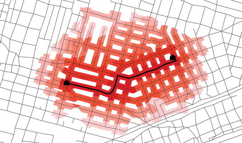Parameter specifies the ‘degree’ of the potential path tree for each pair of control points. Because the amount of total intensity assigned within a given potential path tree varies based on the complexity of the network, this parameter adjusts the intensity to reflect those differences. In practice, it is calculated as the number of unique terminal shortest paths in a potential path tree for two control points. Finally, the intensities for all trees are summed and divided by the number of trees (N-1 control points) to generate the final intensity surface. Figure 2 illustrates a TGDE surface for a simple data set of two control points located on a street network. Note the intensity is higher along the shortest path between locations, as the object could spend the largest amount of time there relative to other locations on the potential path tree.

Figure 2. Distance-weighted potential path tree.

Methods

This section demonstrates the general approach of TGDE for mapping activity spaces of potential criminals given two known anchor points and aggregating them into a single intensity surface representing their combined spaces. However, the basic technique described in the previous section is adapted in two important ways. First, the formulation is modified to create a cumulative intensity surface that combines potential path trees for multiple individuals; in other words densities for individual potential path trees are calculated and combined in a single formula. Second, the equation is altered slightly to fit the more typical scenario of having precise spatial locations for individuals, in the form of home and work anchor points, but lacking any specific temporal information about their movements, in terms of both when they are at home or work and how long their journey to work travel takes. Although the methodology might be best used with actual tracking or travel diary data with timestamps for possible criminals, analysts are unlikely to possess such data. Therefore, a more robust approach is used here, which maps activity spaces as the areas most likely to be accessible to individuals given their known anchor points. This modified equation can be formulated as

(2)

where:

the cumulative density estimate at any location x on a network,

= the number of individuals in the data set,

= the number of control points in an individual’s data set (two in this case), where consecutive points are denoted and

= distance weighting function of potential path tree,

= shortest path distance between any two locations on a network,

= fixed discretionary travel distance, and

= degree of potential path tree.

The two differences between the TGDE approaches are expressed in the equations, with other parameters as previously described. First, Equation (2) calculates a cumulative density based on summing the potential path trees of number of individuals rather than just one. It does so by summing the weighted potential path trees for all individuals and dividing by the total number of individuals in the data set, creating an average intensity for each location in the map. Second, the term from Equation (1) is replaced by the term , which also specifies the maximum possible travel distance between control points. It does so by adding a fixed amount of discretionary travel to the shortest path distance between a pair of control points as per Downs (2014). For example, if the shortest path between two control points is 2 km, then 1 km could be added to that amount to generate a potential path tree that includes the shortest path and all other locations that can be reached in a total distance of 3 km while still anchored to both control points. In this way, potential path trees can be used to map activity spaces of individuals given known home and work locations and an estimated travel budget of a particular distance. While it does not measure when those locations might be occupied, it does provide a useful way to estimate offender activity spaces knowing that they likely travel between home and work regularly. The approach is applied to a database of home and work addresses of registered sex offenders in the City of St. Louis, and it is compared to locations of known rape incidents in the city for a comparable time frame.

Study area & data

The City of St. Louis was selected as the study area for this research because, like other states, Missouri requires convicted sex offenders to register with law enforcement agencies upon their release. In Missouri, offenders must report both their home and work addresses to the Missouri Sex Offender Registry (MSOR) and update them any time there is a change in either. This requirement is designed to make the public aware of convicted sex offenders living or working in their neighbourhoods, as well as helps law enforcement keep track of previous offenders in the event that any reoffend. This situation provides a unique database for testing the modified TGDE approach, since paired home and work locations are available for a number of individuals potentially at risk of committing future crimes.

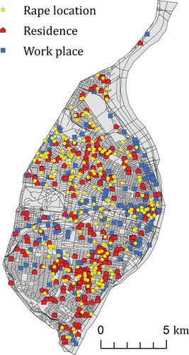
The MSOR is maintained by the Missouri State Highway patrol. In this study, only offenders that had both work and home addresses in St. Louis City were downloaded for inclusion in the analysis. The database was accessed on 25 May 2013. Furthermore, only offenders that had committed forcible or attempted rape (including sodomy) were included in this analysis. The work and home addresses of each individual were geocoded using a GIS (ArcMap v. 10.1, ESRI Inc.) with a 99% success rate, resulting in 87 pairs of home and work locations. Known forcible or attempted rape (including sodomy) incidents in St. Louis during 2012 were also mapped for comparison. The incident reports, which included the spatial coordinates for the majority of events, were obtained from the St. Louis Metropolitan Police Department. A total of 243 locatable incidents fell within the city boundary and were included in the analysis. Figure 3 shows the rape incidents with respect to the home and workplaces of the sex offenders. Basic spatial data layers representing streets in the city and administrative boundaries were downloaded from the U.S. Census Bureau (www.census.gov).

Figure 3. Registered sex offender homes and workplaces in St. Louis mapped with respect to rape incidents.

Although St. Louis was chosen as the study area because of data availability, it is also an interesting city in terms of crime analysis. St. Louis is the second largest city in Missouri, and has a total population of about 320,000 people. The city is well studied in terms of its economic and racial segregation (see Farley 1983, 1995, 2005), and violent crime and burglary rates are considerably higher there than the national average for metropolitan areas (Rountree and Land 2000). Crimes patterns of various types are described in a variety of manuscripts (e.g. Kubrin and Weitzer 2003; Watkins and Decker 2007; Mares 2013).

Analysis

Final TGDE intensity surfaces were generated from the paired home and work locations for the 87 sex offenders in the study sample. Intensities were calculated for each node in the street network (n = 9271). Three surfaces were created for comparison using different values for the parameter measuring the additional discretionary travel distance: 250, 500, and 1000 meters. These values were chosen to represent a range of travel patterns ranging from very restricted movement near the shortest path between home and work to more flexible activity away from this route. The calculations were performed using a standard set of functions in the Network Analyst Extension for ArcMap GIS. First, relevant shortest path network distances needed for Equation (2) were calculated: the distance between each home location and node in the network, the distance between each workplace and node, and the distance between each individual’s home and workplace. The results were joined into a larger attribute table containing all of the distances organised by network node and individual. Second, the degree of the shortest path tree was calculated for each individual. This was accomplished by counting the number of unique shortest paths in each potential path tree. Unique paths were identified as having different total lengths. The calculated potential path tree degrees were also joined to the larger attribute table containing relevant distances. Third, TGDE Equation (2) was applied using a field calculator in the attribute table. Once these intensity values were calculated for each node in the network, they were interpolated to continuous space using a Voronoi diagram. A Voronoi diagram is a spatial tessellation widely used in GIS that assigns each location in space to the nearest input point (Okabe et al. 2000). In this case, all locations in the city are assigned to the nearest network node, which also gives them the intensity value of that node. This process also facilities geovisualisation of the intensity values. Intensities were mapped using a quintile classification scheme.

The intensity surfaces quantifying the areas most accessible to sex offenders were compared to observed rape incident data to evaluate how well they predict crime. First, the rape incidents were spatially joined with the TGDE surfaces to identify the intensity value at each location. The calculated intensities were multiplied by a scaling factor of 1 x 10³ to reduce excessive decimals, as is common for density estimation techniques. Summary statistics were reported for each of the three surfaces. Second, those values were compared to random points (1,000 sets of 243 random incidents). Random points were not generated inside Census tracts that had zero population if rapes were not observed there to avoid artificially biasing the results towards areas with little expected crime. The northernmost Census tracts of low population density were also excluded for the same reason. The results were compared using a Kolmorogov–Smirnov test. This nonparametric test was used since the intensity values were not normally distributed in either sample. The purpose of the comparison was to determine whether the rape incidents were at locations with higher intensity values than recorded for random locations. If this was the case, then it was concluded that TGDE intensity surfaces derived from sex offender activity spaces effectively predicted the locations of rapes.

Results

Final TGDE surfaces representing estimated sex offender activity spaces with different discretionary travel distances in St. Louis are shown in Figure 4. About 68% of the city is covered by the interpolated potential path trees under the lowest travel budget scenario of 250 m. The highest intensity areas were found mostly in the eastern and central parts of the city, while those outside this area mostly occurred in residential areas in the southwest and north. The high-intensity areas occurred mostly along the shortest paths between offender home and work, since the estimated travel budget is quite restrictive. About 90% of the observed rape incidents occurred within the activity spaces of the offenders, while only 67.5% of random points fell within the same region. The incidents had a median (scaled) intensity of 0.0044 with a mean value of 0.038. The median was almost twice that for random points ( = 0.0023), which had a mean value of 0.015. The Kolmorogov–Smirnov test indicated the differences in medians was significant (, meaning that intensities were greater at rape incident locations than expected by random.

Figure 4. TGDE surfaces representing estimated sex offender activity spaces in St. Louis using three discretionary travel budgets of 250 m (a), 500 m (b), and 1000 m (c).

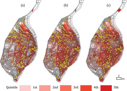
Intensity maps for the larger discretionary travel distances produce much the same general pattern but encompass greater proportions of the city. The top quintiles of intensity occur within the same areas of eastern and central St. Louis as the 250 m analysis, but more pronounced high-intensity areas also occur in the western part of the city. As the travel budget increases, the high-intensity areas are less linearly shaped compared to the smaller distances. Using the 500 m and 1000 m distances, 78% and 87% of the city occur within the activity spaces, along with the same percentages of random points. For the 500 m scenario, 95.5% of the rape incidents occurred within the activity spaces of the offenders. The median intensity for the incident sites was 0.0078 with a mean of 0.038. This compares to a median intensity at random points of 0.0050 and a mean of 0.0166. For the 1000 m scenario, 98% of the rape incidents occurred within the potential path trees. The rape sites not captured by the potential path trees were located in the northwest part of the city. The median intensity for the incident sites was 0.0027 with a mean of 0.111. This compares to a median intensity at random points of 0.0021 and a mean of 0.058. The Kolmorogov–Smirnov test indicated the differences in medians for both scenarios were significant (.

Discussion

The three TGDE surfaces representing combined sex offender activity spaces produced relatively similar results regarding predicting rape locations in St. Louis. Although large percentages of the city fell within the potential path trees of offenders, areas of high intensity were confined to much smaller regions. All three discretionary travel distance scenarios identified roughly the same highest intensity areas in eastern and central St. Louis – particularly in the downtown area – although some smaller regions were more pronounced under the higher distance scenarios. Although all three maps produced significantly higher intensities at rape locations compared to random points, indicating predictive power, it is desirable to assess which scenario might be the most accurate or useful.

There is a trade-off between capturing higher percentages of incident sites and more precisely delineating the at-risk activity spaces, which may be important for targeting policing efforts. As larger discretionary travel distances are used, potential path trees encompass more of the city – potentially extending beyond the study area boundaries if large enough values are used – and the intensity surface becomes much smoother. Larger distance values allow more incident sites to be captured but at the expense of including more areas without observed rapes within the activity spaces; as distances increase, high-intensity areas visible at smaller distances merge together into a larger, more homogenous region. One way of evaluating the predictive power of each map is to calculate the ratio of the median intensities between rape sites and random points, with larger ratios indicating better performance. In this study, the calculated ratios are 1.87, 1.54, and 1.35, in order of increasing distance. As discretionary distances are increased beyond those reported in this paper, the relationship between the activity spaces and rape incident weakens, meaning the smallest travel distance scenario best predicts rape incidents. This is interesting, as it suggests rape incidents are concentrated on and very close to the anchor points and expected travel paths of sex offenders, which is consistent with the journey-to-crime literature (Andresen, Frank, and Felson 2014). In terms of policing, relationship is helpful to exploit, as the effectiveness of a crime prediction technique can be measured by comparing the sizes of search areas to the overall study area (Rossmo 2005).

The main advantage of this particular mapping approach is that it allows one to predict crimes based on the estimated activity spaces of potential criminals. In this way it models the mechanism creating the pattern of crime, namely the movements of potential criminals seeking possible victims from available opportunities within a city. In the case study presented in this paper, activity spaces estimated for 87 convicted sex offenders both working and residing in St. Louis were sufficient to predict the spatial patterns of rape. There are three main explanations for the effectiveness of the approach. First, one might infer that the individuals in the data set were responsible for committing the 243 known forcible or attempted rapes (including sodomy) analysed in the study. However, this explanation is unlikely given the number of incidents and the fact that recidivism rates for convicted sex offenders are relatively low compared to other types of crime (Langan and Levin 2002; Bonner-Kidd, 2010; Tewksbury, 2012). Furthermore, some of the offenders were released after many of the crimes were actually committed, given that the offender database was accessed in 2013, while the rape data is from 2012.

A more reasonable second explanation is that the estimated activity spaces of the sex offenders are representative of people likely to commit rape or sodomy. Other research has found that sex crimes are more likely to be committed by people with prior criminal records (Langan, Schmitt, and Durose 2003). And, in general, people with criminal records – whether for sex crimes or other offenses – have much more limited housing and employment options than the general public (Berenson and Appelbaum 2011; Socia 2011; Grubesic 2010; Grubesic, Murray, and Mack 2011). For these reasons, activity patterns of the population at risk for committing rape might be approximated by that of convicted sex offenders. Third, one could also argue that the potential path trees generated in this paper are representative of the general population in St. Louis and predict crime patterns for that reason. However, given that the home and work locations of sex offenders are clustered in the city (Figure 2), as their housing and employment options are limited due to residence restriction laws (Missouri Statute §589.417), this is unlikely to be the case. Furthermore, several highly populated neighbourhoods in the city occur outside the estimated activity spaces and show few to no rapes. The second argument most likely explains the effectiveness of the time-geographic approach in this case study.

While the final TGDE surfaces created from estimated activity spaces were able to predict rape locations, there are some limitations to the approach that should be noted. First, the intensity maps were based on sex offender activity spaces that were calculated solely from their home and work addresses and estimated discretionary travel distances. In reality, individuals may choose alternate routes than those estimated by the shortest path between home and work, for instance if they have routine intermediate stops at more distant locations. Additionally, different individuals will have different travel budgets depending on their mobility or time flexibility. The approach used in this study produced the best estimate of activity spaces given limited information of two anchor points. However, the approach could be improved with more detailed data, such as that collected by tracking released offenders using GPS. This would add an explicit temporal component to the data (such as working hours), which would allow the activity spaces and resulting TGDE surface to be generated much more precisely.

Second, the time-geographic approach predicts crime based on estimated criminal activity spaces but does not assess opportunities available to individuals, which also contribute to crime rates and may be distributed unevenly across space. Thus, this approach may be more predictive when combined with other ancillary data that represent opportunities attractive to criminals or areas that are already vulnerable. Some of these factors might include the abundance of potential victims, proportion of socially vulnerable persons (Alaniz, Cartmill, and Parker 1998), accessibility to alcohol outlets (Block and Block 1995; Brower and Carroll 2007), low light conditions at night (Pain et al. 2006), or low law enforcement presence. If the intensity map is overlaid by these types of data, it could be used to identify where expected criminal movements coincide with potential opportunities, thereby identifying locations important for targeting preventative policing strategies (Warburton and Shepherd 2004; Chainey, Tompson, and Uhlig 2008; Taylor, Koper, and Woods 2011; Ratcliffe et al. 2011). It is hoped that the general methodology will be useful for predicting not only rapes but also other types of crimes, such as burglaries, or for other applications where potential path areas are used to estimate activity spaces.

Disclosure statement

No potential conflict of interest was reported by the author.

Additional information

Funding

Portions of this research were funded by grants made to the authors from the National Science Foundation (NSF) [grant number BCS-1062947]. The contents of this article are the responsibility of the author and do not reflect the views of the NSF.

References

- Alaniz, M. L., R. S. Cartmill, and R. N. Parker. 1998. “Immigrants and Violence: The Importance of Neighborhood Context.” Hispanic Journal of Behavioral Sciences 20: 155–174. doi:10.1177/07399863980202002.
- Andresen, M. A., R. Frank, and M. Felson. 2014. “Age and the Distance to Crime.” Criminology and Criminal Justice 14 (3): 314–333. doi:10.1177/1748895813494870.
- Bailey, T. C., and A. C. Gatrell. 1995. Interactive Spatial Data Analysis, 432 pp. Harlow: Longman Scientific & Technical; New York: J. Wiley.
- Berenson, J., and P. S. Appelbaum. 2011. “A Geospatial Analysis of the Impact of Sex Offender Residency Restrictions in Two New York Counties.” Law and Human Behavior 35: 235–246. doi:10.1007/s10979-010-9235-3.
- Block, R., and C. Block. 1995. “Space, Place and Crime: Hot Spot Areas and Hot Places of Liquor-Related Crime.” In Crime and Place, edited by J. E. Eck and D. Weisburd, 145–183. Monsey, NY: Criminal Justice Press; Washington, DC: Police Executive Research Forum.
- Bonnar-Kidd, K. K. 2010. “Sexual Offender Laws and Prevention of Sexual Violence or Recidivism.” American Journal of Public Health 100: 412–419. doi:10.2105/AJPH.2008.153254.
- Brantingham, P., and P. Brantingham. 1993. “Environment, Routine, and Situation: Toward a Pattern Theory of Crime.” In Routine Activity and Rational Choice, Advances in Criminological Theory. Vol. 5, edited by R. Clarke and M. Felson. New Brunswick, NJ: Transaction Publishers.
- Brower, A. M., and L. Carroll. 2007. “Spatial and Temporal Aspects of Alcohol-Related Crime in a College Town.” Journal of American College Health 55 (5): 267–275.
- Chainey, S., L. Tompson, and S. Uhlig. 2008. “The Utility of Hotspot Mapping for Predicting Spatial Patterns of Crime.” Security Journal 21: 4–28. doi:10.1057/palgrave.sj.8350066.
- Cohen, L. E., and M. Felson. 1979. “Social Change and Crime Rate Trends: A Routine Activity Approach.” American Sociological Review 44: 588–60. doi:10.2307/2094589.
- Downs, J. A. 2010. “Time-Geographic Density Estimation for Moving Point Objects.” Lecture Notes in Computer Science 6292: 16–26.
- Downs, J. A. 2014. “Using Potential Path Trees to Map Sex Offender Access to Schools.” Applied Spatial Analysis and Policy 7: 381–394. doi:10.1007/s12061-014-9116-0.
- Downs, J. A., and M. W. Horner. 2012. “Probabilistic Potential Path Trees for Visualizing and Analyzing Vehicle Tracking Data.” Journal of Transport Geography 23: 72–80. doi:10.1016/j.jtrangeo.2012.03.017.
- Downs, J. A., M. W. Horner, G. Hyzer, D. Lamb, and R. Loraamm. 2014. “Voxel-Based Probabilistic Space-Time Prisms for Analysing Animal Movements and Habitat Use.” International Journal of Geographical Information Science 28: 875–890. doi:10.1080/13658816.2013.850170.
- Downs, J. A., M. W. Horner, and A. Tucker. 2011. “Time-Geographic Density Estimation for Home Range Analysis.” Annals of GIS 17 (3): 37–41.
- Farley, J. E. 1983. “Metropolitan Housing Segregation in 1980: The St. Louis Case.” Urban Affairs Review 18: 347–359. doi:10.1177/004208168301800304.
- Farley, J. E. 1995. “Race Still Matters: The Minimal Role of Income and Housing Cost as Causes of Housing Segregation in St. Louis, 1990.” Urban Affairs Review 31: 244–254. doi:10.1177/107808749503100207.
- Farley, J. E. 2005. “Race, Not Class: Explaining Racial Housing Segregation in the St. Louis Metropolitan Area, 2000.” Sociological Focus 38: 133–150. doi:10.1080/00380237.2005.10571261.
- Grubesic, T., A. Murray, and E. Mack. 2011. “Sex Offenders, Residence Restrictions, Housing, and Urban Morphology: A Review and Synthesis.” Cityscape 13: 7–31.
- Grubesic, T. H. 2010. “Sex Offender Clusters.” Applied Geography 30: 2–18. doi:10.1016/j.apgeog.2009.06.002.
- Hägerstrand, T. 1970. “What About People in Regional Science?” Papers in Regional Science 24: 7–21. doi:10.1111/j.1435-5597.1970.tb01464.x.
- Harding, C., Z. Patterson, L. F. Miranda-Moreno, and S. A. H. Zahabi. 2012. “Modeling the Effect of Land Use on Activity Spaces.” Transportation Research Record: Journal of the Transportation Research Board 2323: 67–74. doi:10.3141/2323-08.
- Horner, M. W., and J. A. Downs. 2014. “Integrating People and Place: A Density-Based Measure for Assessing Accessibility to Opportunities.” Journal of Transport and Land Use 7 (2): 23–40. doi:10.5198/jtlu.v7i2.
- Horner, M. W., B. Zook, and J. A. Downs. 2012. “Where Were You? Development of a Time-Geographic Approach for Activity Destination Re-Construction.” Computers, Environment and Urban Systems 36: 488–499. doi:10.1016/j.compenvurbsys.2012.06.002.
- Kamruzzaman, M., J. Hine, B. Gunay, and N. Blair. 2011. “Using GIS to Visualise and Evaluate Student Travel Behaviour.” Journal of Transport Geography 19 (1): 13–32. doi:10.1016/j.jtrangeo.2009.09.004.
- Kestens, Y., A. Lebel, M. Daniel, M. Thériault, and R. Pampalon. 2010. “Using Experienced Activity Spaces to Measure Foodscape Exposure.” Health & Place 16 (6): 1094–1103. doi:10.1016/j.healthplace.2010.06.016.
- Kubrin, C. E., and R. Weitzer. 2003. “Retaliatory Homicide: Concentrated Disadvantage and Neighborhood Culture.” Social Problems 50: 157–180. doi:10.1525/sp.2003.50.2.157.
- Kuijpers, B., R. Grimson, and W. Othman. 2011. “An Analytic Solution to the Alibi Query in the Space–Time Prisms Model for Moving Object Data.” International Journal of Geographical Information Science 25: 293–322. doi:10.1080/13658810902967397.
- Kuijpers, B., H. J. Miller, T. Neutens, and W. Othman. 2010. “Anchor Uncertainty and Space-Time Prisms on Road Networks.” International Journal of Geographical Information Science 24: 1223–1248. doi:10.1080/13658810903321339.
- Kwan, M. 1999. “Gender, the Home‐Work Link, and Space‐Time Patterns of Nonemployment Activities.” Economic Geography 75: 370–394. doi:10.2307/144477.
- Langan, P., and D. Levin. 2002. “Recidivism of Prisoners Released in 1994.” Federal Sentencing Reporter 15 (1): 1–16.
- Langan, P., E. Schmitt, and M. Durose. 2003. Bureau of Justice Statistics Recidivism of Sex Offenders Released from Prison in 1994. Vol. 59, 1–49. NCJ 198281. http://www.bjs.gov/content/pub/pdf/rsorp94.pdf
- Mares, D. 2013. “Climate Change and Crime: Monthly Temperature and Precipitation Anomalies and Crime Rates in St. Louis, MO 1990-2009.” Crime Law and Social Change 59: 185–208. doi:10.1007/s10611-013-9411-8.
- Martinez, A. N., J. Lorvick, and A. H. Kral. 2014. “Activity Spaces among Injection Drug Users in San Francisco.” International Journal of Drug Policy 25 (3): 516–524. doi:10.1016/j.drugpo.2013.11.008.
- Mason, M. J., and K. Korpela. 2009. “Activity Spaces and Urban Adolescent Substance Use and Emotional Health.” Journal of Adolescence 32 (4): 925–939. doi:10.1016/j.adolescence.2008.08.004.
- Miller, H. J. 2005a. “Necessary Space - Time Conditions for Human Interaction.” Environment and Planning B: Planning and Design 32: 381–401. doi:10.1068/b31154.
- Miller, H. J. 2005b. “A Measurement Theory for Time Geography.” Geographical Analysis 37: 17–45. doi:10.1111/gean.2005.37.issue-1.
- Morgan, J., and P. Steinberg. 2013. “Testing the Usability of Time-Geographic Maps for Crime Mapping.” Geotechnologies and the Environment 8: 339–366.
- Okabe, A., B. Boots, K. Sugihara, and S. N. Chiu. 2000. Spatial Tessellations: Concepts and Applications of Voronoi Diagrams. 2nd ed. Series in Probability and Statistics. Chichester: Wiley.
- Pain, R., R. MacFarlane, K. Turner, and S. Gill. 2006. ““When, Where, If, and But”: Qualifying GIS and the Effect of Streetlighting on Crime and Fear.” Environment and Planning A 38: 2055–2074. doi:10.1068/a38391.
- Patterson, Z., and S. Farber. 2015. “Potential Path Areas and Activity Spaces in Application: A Review.” Transport Reviews 35 (6): 1–22.
- Paulsen, D. J., S. Bair, and D. Helms. 2009. Tactical Crime Analysis: Research and Investigation, 240 pp. Boca Raton, FL: CRC Press.
- Ratcliffe, J. H. 2006. “A Temporal Constraint Theory to Explain Opportunity-Based Spatial Offending Patterns.” Journal of Research in Crime and Delinquency 43: 261–291. doi:10.1177/0022427806286566.
- Ratcliffe, J. H., T. Taniguchi, E. R. Groff, and J. D. Wood. 2011. “the Philadelphia Foot Patrol Experiment: A Randomized Controlled Trial of Police Patrol Effectiveness in Violent Crime Hotspots.” Criminology 49: 795–831. doi:10.1111/crim.2011.49.issue-3.
- Rossmo, D. K. (2005). An evaluation of NIJ’s evaluation methodology for geographic profiling software. Accessed 18 January 2016. http://www.ojp.usdoj.gov/nij/maps/gp.html.
- Rountree, P. W., and K. C. Land. 2000. “The Generalizability of Multilevel Models of Burglary Victimization: A Cross-City Comparison.” Social Science Research 29: 284–305. doi:10.1006/ssre.2000.0670.
- Sherman, J., J. Spencer, J. Preisser, W. M. Gesler, and T. A. Arcury. 2005. “A Suite of Methods for Representing Activity Space in A Healthcare Accessibility Study.” International Journal of Health Geographics 4 (1): 1–21. doi:10.1186/1476-072X-4-24.
- Sherman, L., P. Gartin, and M. Buerger. 1989. “Hot Spots of Predatory Crime: Routine Activities and the Criminology of Place.” Criminology 27: 27–56. doi:10.1111/crim.1989.27.issue-1.
- Silverman, B. 1986. Density Estimation for Statistics and Data Analysis, 175 pp. London: CRC Press.
- Socia, K. M. 2011. “The Policy Implications of Residence Restrictions on Sex Offender Housing in Upstate NY.” Criminology & Public Policy 10: 351–389. doi:10.1111/capp.2011.10.issue-2.
- Taylor, B., C. Koper, and D. Woods. 2011. “A Randomized Controlled Trial of Different Policing Strategies at Hot Spots of Violent Crime.” Journal of Experimental Criminology 7: 149–181. doi:10.1007/s11292-010-9120-6.
- Tewksbury, R. 2012. “A Longitudinal Examination of Sex Offender Recidivism Prior to and following the Implementation of SORN.” Behavioral Sciences & the Law 328: 308–328. doi:10.1002/bsl.1009.
- Villanueva, K., G.-C. Billie, M. Bulsara, G. McCormack, A. Timperio, N. Middleton, B. Beesley, and G. Trapp. 2012. “How Far Do Children Travel from Their Homes? Exploring Children’s Activity Spaces in Their Neighborhood.” Health & Place 18 (2): 263–273. doi:10.1016/j.healthplace.2011.09.019.
- Warburton, A., and J. Shepherd. 2004. “Development, Utilisation, and Importance of Accident and Emergency Department Derived Assault Data in Violence Management.” Emergency Medicine Journal 24 (4): 473–478.
- Watkins, A. M., and S. H. Decker. 2007. “Patterns of homicide in East St. Louis.” Homicide Studies 11: 30–49. doi:10.1177/1088767906296020.
- Winter, S., and Z.-C. Yin. 2010. “Directed Movements in Probabilistic Time Geography.” International Journal of Geographical Information Science 24: 1349–1365. doi:10.1080/13658811003619150.
- Yuill, R. S. 1971. “The Standard Deviational Ellipse; an Updated Tool for Spatial Description.” Geografiska Annaler. Series B. Human Geography 53 (1): 28–39. doi:10.2307/490885.
- Zenk, S. N., A. J. Schulz, S. A. Matthews, A. Odoms-Young, J. Wilbur, L. Wegrzyn, K. Gibbs, C. Braunschweig, and C. Stokes. 2011. “Activity Space Environment and Dietary and Physical Activity Behaviors: A Pilot Study.” Health & Place 17 (5): 1150–1161. doi:10.1016/j.healthplace.2011.05.001.