A new research paradigm for global land cover mapping

ABSTRACT

In this paper, we introduced major challenges in mapping croplands, settlements, water and wetlands, and discussed challenges in the use of multi-temporal and multi-sensor data. We then summarized some of the on-going efforts in improving qualities of global land cover maps. Existing technologies provide sufficient data for better map making if extra efforts can be made instead of harmonizing and integrating various global land cover products. Developing and selecting better algorithms, including more input variables (new types of data or features) for classification, having representative training samples are among conventional measures generally believed effective in improving mapping accuracies at local scales. We pointed out that data were more important in improving mapping accuracies than algorithms. Finally, we proposed a new paradigm for global land cover mapping, which included a view of vegetation classes based on their types and form, canopy cover and height. The new paradigm suggests that a universally applicable training sample set is not only possible but also effective in improving land cover classification at the continental and global scales. To ensure an easy transition from traditional land cover mapping to the new paradigm, we recommended that an all-in-one data management and analysis system be constructed.

KEYWORDS:

• Remote sensing
• image classification
• class definition
• universal sampling
• all-in-one system
• on-line mapping

1. Progresses of global land cover mapping

Global land cover mapping originated from traditional surveying and mapping. Before the advent of satellite remote sensing in the 1960s, the surface of Earth had never been completely mapped at relatively fine spatial scales and consistent time periods. For example, until 2005, China still had approximately 1/5th of its territory unmapped at the scale of 1:50,000 with topographical mapping standard. Since the launch of the first land observation satellite in 1972, the Earth surface began to be imaged at approximately 80-m resolution, which was improved to 30 m with the advent of Landsat Thematic Mapper (TM) data in 1982 and then to 10-m resolution with the advent of Satellite Pour l’Observation de la Terre (SPOT) High Resolution Visible (HRV) data in 1986. Despite these advances, the complete coverage of the Earth surface takes years to complete in the early years following the launch of Landsat and SPOT satellites. It is not until the late 1990s when Landsat 7 was launched, relatively consistent and systematic global data coverage at 30-m resolution over the Earth surface began to become available.

Initial global land cover mapping was done with processed weather satellite data products, primarily from Advanced Very High Resolution Radiometer (AVHRR) data acquired on board National Oceanic and Atmospheric Administration (NOAA) weather satellite series. The resolution of AVHRR data are coarser than 1 km. Since the primary goal was to use land cover data in land process models in support of climate change studies, global land cover data products at 1–100-km level are acceptable (e.g. DeFries and Townshend 1994; Loveland and Belward 1997). Since the launch of the Earth Observation System in 1999, annual global land cover has been produced at the 500-m resolution level with the Moderate Resolution Imaging Spectrometer (MODIS) data (Friedl et al. 2002). While there has been a number of sub-kilometre level global land cover data products developed by the global scientific research community, the first 30-m resolution global land cover dataset, Finer Resolution Observation and Monitoring of Global Land Cover (FROM-GLC), has been produced with circa 2010 Landsat data in 2011 (Gong et al. 2013). FROM-GLC is the only global land cover product that contains a hierarchical structure of classes. At its first level, it contains 10 broad land cover categories, and at the second level they are further broken into 29 more detailed classes. FROM-GLC also features a unique equal area stratified random sample set for validation purposes. The locations of FROM-GLC validation sample units are openly available to the public, making it possible for refinement through international collaboration.

Despite the fact that there have already been a handful number of global land cover products – most of them are prepared primarily to meet the purpose of land process modelling – a component in climate system studies. Although there have been recent discussions on the need for global land cover data for biodiversity and agricultural management purposes (Fritz et al. 2015; Skidmore et al. 2015), few efforts have been made to meet such needs. An exception is the global cropland map –Finer Resolution Observation and Monitoring-Global Cropland (Yu et al. 2013), which is a single-class land cover mask lacking accuracy (in the order of 60%) and sufficient level of specific subclasses (e.g. major crop species). Grain yield forecasting requires more specific and accurate data on crop species distribution.

Global land cover is an important variable for climate change and sustainable development studies (Yang et al. 2013; Xu et al. 2013). In the 12th Group on Earth Observation (GEO) Plenary and Mexico City Ministerial Summit held in November, 2015, the needs for global land cover data products in support of the United Nations Sustainable Development Goals (SDG) have been discussed. Finer resolution global land cover data products available to various nations with flexible land cover classification schemes are needed in support of the social and economic applications. This represents a new demand for land cover data both at the global and national scales. Clearly, the land cover mapping community is not yet prepared to meet this need. Meeting this need requires not only technological advancements but also re-thinking of mapping approaches based on the specific characteristics of global mapping and more effective international collaboration. In the remaining of this paper, we use examples to illustrate some of the challenges in mapping land cover at the global scale, followed by a perspective to future research directions.

2. Challenges

Global land cover mapping at relatively fine resolution has many difficulties. There are three common difficulties. First, the mapping purpose could vary drastically with different applications. Different application requires different classification scheme. Therefore, a land cover map with a fixed set of class categories may not meet the needs other than it is proposed for. In addition, one cannot design a classification scheme that meets the need of a particular application without checking whether there is sufficient separability among the classes given the type of remotely sensed data at hands. Previous experiences indicate that with optical data alone, it is very difficult to achieve land cover mapping accuracies better than 80% even with under a dozen level-1 land cover classes at the global scale. Second, input features play a significant role in land cover mapping (Li et al. 2014; Yu, Liang, et al. 2014). Microwave, thermal and light detection and ranging (LiDAR)-based vegetation-height data could help further improve accuracies. However, there is currently no wall-to-wall map of vegetation height data available. Neither microwave nor thermal data has been integrated into optical data in land cover mapping at the global scale. Third, it takes years for an individual image analyst to collect enough training data for the entire globe. It is impossible for an individual to visit all needed sites for ground truth. Therefore, mapping global land cover requires close collaboration of multiple image analysts. Their consistencies in standards and complementary knowledge in being familiar with different parts of the world are extremely important.

From previous land cover mapping experiences, it has been reported that some land cover categories tended to have low classification accuracies. These included wetland, shrubland, human settlements and croplands (Sulla-Menashe et al. 2011; Gong et al. 2013). Although water can be classified at an accuracy better than 80%, which is comparably well classified than most other classes in many global land cover products, a recent study revealed that a number of common factors (e.g. cloud and mountain shadow) influencing other land cover categories also influence water (Ji et al. 2015). Therefore, substantial improvement is possible in water mapping. In the following, we present some examples illustrating the difficulties in global land cover mapping over specific regions or for cropland, human settlements, water and wetlands. Shrubland is a transitional category between grassland and forest land. As shall be explained in Section 4.1, it requires more quantitative information to better define/characterize it.

2.1. Limitations in global cropland mapping and two case studies in tropical region

Precise estimation of cropland (including plantation) extent for the entire world is crucial for water resource planning, food security research, Earth system and global change studies (Thenkabail et al. 2010; Gong et al. 2013). Current global cropland products based on remote sensing face many limitations (see Table 1).

Table 1. Uncertainties and future improvements suggested by the developers of the four global cropland products produced using remote sensing data.

	Uncertainties	Future improvements
Thenkabail et al. (2009)	(1) Inconsistency in the national census data on how irrigated areas are compiled, (2) resolutions and/or scales at which the irrigated area statistics are derived and (3) definition issues.	Use of finer resolution data (Thenkabail et al. 2010)
Biradar et al. (2009)	(1) Methods and approaches, (2) definitions, (3) uncertainties in rainfed area fractions, (4) resolutions or scales	Not clearly put forward
Pittman et al. (2010)	Not clearly put forward	Moving from static to dynamic monitoring applications in the next step of global cropland mapping
Yu et al. (2013)	(1) Cloud cover; (2) area with small cropland size; (3) rice area	(1) Multi-temporal Landsat TM/enhanced TM+ images, (2) Synthetic Aperture Radar dataset with global coverage, (3) sample expansion for cropland
Summary	(1) Definition; (2) map uncertainties (spatial distribution and types); (3) resolutions issues; (4) quality of inventory data; (5) image processing and methods	(1) Higher spatial resolution; (2) more frequent data; (3) inclusion of non-optical sensors; (4) more reliable samples

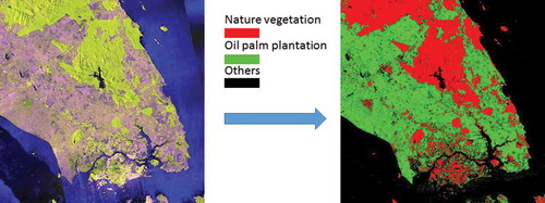
We present two case studies to demonstrate the limitations and possible improvements for better cropland mapping. Cloud cover (and accompanying shadows) is a troublesome issue for using optical data. According to the estimation from Eastman, Warren, and Hahn (2013), the average (day and night) frequency of occurrence of completely clear sky is only 20.7% for the whole world, and tropical (especially Indonesia islands) and polar regions are the areas with very low clear sky occurrence. As a result, underestimation of cropland areas in the tropics regions was observed (Yu et al. 2013). Multi-temporal optical images can help reduce cloud effects (Yu, Wang, and Gong 2013). However, for some regions (for example, see Figure 1), images in cloud-free-windows are hard to obtain. Most pixels in this region have 40–80% cloud cover. Synthetic Aperture Radar (SAR) data (which can penetrate clouds) offer a solution in such areas. Figure 2 shows an Advanced Land Observing Satellite (ALOS)/Phased Array type L-band SAR (PALSAR) image over the same area as in Figure 1. There is a potential to separate oil palm plantation from natural vegetation (Figure 2), which is difficult for optical remote sensing.

Figure 1. The cloud free proportion statistics using all Landsat imagery for a location (path-125, row-59) covering Malaysia and Singapore.

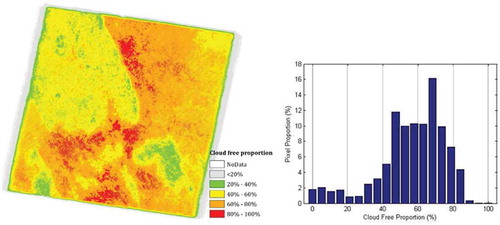
Figure 2. An ALOS/PALSAR image (r-HH, g-HV, b-HH/HV) and the derived oil palm plantation map.

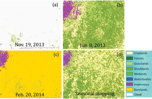
Another example is from a semi-arid location (around Yelwa City, Kebbi State, Nigeria) in the tropics region affected by thick cloud occasionally [see Figure 3(a)], or cloud/shadow misclassified to other land cover types. In Figure 3(b), cloud/shadow at the urban fringe are misclassified as impervious area. This region exhibits two seasons – a short raining season (usually from June to September) and a prolonged dry season (usually from October to May). The most significant obstacle in cropland mapping is distinguishing cropland from other land cover types. Cropland could be mixed with natural vegetation (e.g. grassland and shrublands) in the raining season [see Figure 3(b)] and mixed with bareland in the dry season [see Figure 3(c)]. Seasonal variation in the ‘greenness’ of vegetation described in temporal dynamics of vegetation indices is important for mapping vegetated surfaces. One way to improve the accuracies of global land cover map is to use multi-temporal Landsat/SPOT/Sentinel-2 images. Figure 3(d) shows an improved example using seasonal Landsat images acquired in 2013 and 2014.

Figure 3. Land cover maps derived from Landsat images acquired on different dates for Yelwa City, Kebbi State, Nigeria. (a) 19 November 2013; (b) 8 June 2013; (c) 20 February 2014; (d) derived from images of all seasons.

2.2. Challenge for global mapping of human settlements

According to the latest World Urbanization Prospects (United Nations 2015), more than half of the world’s population resides in urban areas, and this proportion is estimated to reach 66% by 2050. As a consequence, the aggregation of global urban population as well as rapidly expanded human settlement areas, have wide impacts on public health (Gong et al. 2012), forest and biodiversity loss (DeFries et al. 2010; Seto, Güneralp, and Hutyra 2012), and food security (Foley et al. 2011). To cope with these issues, it is of great importance to map the dynamics of global human settlements.

Landsat images are the finest resolution freely accessible over the entire world with a relatively long historical record (over 30 years) and 30-m resolution (Roy et al. 2014). There are two global 30-m human settlement maps. One is an aggregated dataset with multiple sources (Yu, Wang, et al. 2014) and the other is mainly done by human interpretation (Chen et al. 2015). Few attempts have been made to explore efficient methods for automatic mapping of global human settlements with Landsat images. In addition, there lacks continuous track of historical change. Hence, efforts on this topic are urgently needed.

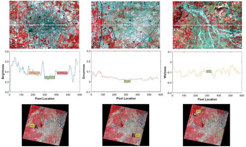
However, global mapping of human settlement area with Landsat image still faces with many challenges. As a special land cover type occupying a tiny fraction on Earth (i.e. less than 1%; Schneider, Friedl, and Potere 2010), globally human settlement areas are composited with complicated structures, materials, densities or spatial forms, which make it easier to be confused with other land cover types based only on their spectral signatures. Figure 4 presents three potential challenges for efficient human settlement extraction from Landsat images. The first is about spatial heterogeneity within the extent of human settlement areas. Figure 4a is Baoding City, located in north China. Although areas within the yellow rectangles are human settlements, their brightness (derived from Tasseled Cap – TC transform) varies considerably among different transections with extremely high or low values. Second, mapping of human settlements in rural areas is easy to be confused with fallow land (Figure 4b). Without vegetation, the greenness of villages and its ambient fallow land are almost the same. Meanwhile, their overall differences are quite low along the entire transect (i.e. white line in Figure 4). Both of them hinder the effectiveness of settlement extraction (Li, Gong, and Liang 2015). The third one is the confusion between human settlement and bareland (Figure 4c), which is a main obstacle documented in many studies (Gao et al. 2012; Jia et al. 2014; Mertes et al. 2015). Areas in Figure 4c are mixed with a small village and a dried river. For these two types, it is hard to distinguish if we only use spectral features.

Figure 4. Challenges in mapping human settlements with Landsat TM images (e.g. scene p123r033). First row: local views composited with bands 4, 3 and 2. Second row: continuous curves of brightness, greenness and wetness (derived from Tasseled Cap transform) along the transect (white line in the 1st row).

Apart from the confusion caused by optical signatures, there are more practical challenges when implementing a global mapping project of human settlements. Urban development is spatially heterogeneous in different regions; image quality may vary scene by scene (i.e. due to cloud contamination and seasonal dynamics or variances of atmospheric conditions). These issues impose a great challenge due to possible inconsistency from local to global scales, particularly for automatic image classification. It may be beneficial to break the global mapping problem into portions according to biogeographic units to avoid the impact of spatial heterogeneity over the world (Schneider, Friedl, and Potere 2010). In addition, isolating human settlements by finding ways to mask out non-settlements could substantially save computation. Finally, features reflecting human gathering such as night lights that can be directly observed from satellites can be incorporated into the mapping of human settlement (Elvidge et al. 2007). On the ground, as more and more open-source social data (e.g. point of interest (POI); open street map) become accessible, they could be useful to improve global mapping of human settlements (Goodchild 2007; Hu et al. 2016).

2.3. Main difficulties in water extraction

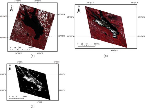
Surface water area is an important variable for water resource management and wildlife conservation. At the local scale, it is considered an easy task to identify water. However, at the global scale, due to the various stages of freezing and melting of water and different lighting conditions, their spectral characteristics vary in space and time (Ji et al. 2015). First is the misclassification between water and shadow. Cloud and mountain shadows (especially when covered with snow or ice) are easily misclassified as water (Figure 5). Cloud shadow could be detected based on its geometric relationship with the cloud by utilizing the view angle of the satellite sensor, the solar zenith and azimuth angle, and the relative height of the cloud. Mountain shadows can be removed by using topographic information, because water bodies are usually distributed on flat terrain.

Figure 5. (a) The false colour of Landsat 8 image with path = 193, row = 028 and day of year (DOY) = 1 (2014). (b) The water map from CFmask (Zhu and Woodcock 2012).

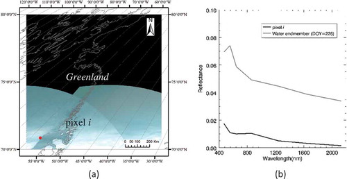
Second, in high-latitude regions, because of the polar night phenomenon, the reflectance data could be much lower than the normal water reflectance, as shown in Figure 6a. Moreover, the land cover type in these areas during polar nights is snow/ice, whose spectral shapes are similar to that of water (Figure 6b). As a result, these areas may all be misclassified as water. Therefore, the beginning and ending day of the polar night period should be detected to exclude those misclassified water areas.

Figure 6. (a) The false colour of Moderate Resolution Imaging Spectrometer (MODIS) image with h = 16, v = 01 and DOY = 30 (2014). (b) the spectral signature of pixel i in (a), and the reference is the spectrum of water endmember extracted from the MODIS image with the same h and v when DOY = 226.

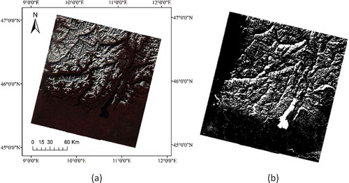
Third, if the altitude angle of the sensor is equal to that of the Sun and they are on the same plane, specular reflection happens leading to very high water reflectance (Figure 7). Such water pixels (Figure 7b) could be easily misclassified as cloud. For these areas, we need to use time-series data to solve this problem.

Figure 7. (a) The false colour of Landsat 8 image with path = 182, row = 017 and DOY = 180 (2014). (b) The false colour of MODIS image with h = 19, v = 02 and DOY = 180 (2014). White areas in the lake are due to mirror-reflection of water. (c) The cloud mask in the MOD09GA package that included mirror reflection areas as cloud.

2.4. Challenges for wetland remote sensing

Timely and reliable information on the status of wetlands at the global scale is critical to a number of important applications, such as biodiversity protection and carbon sequestration. However, due to the highly variable water condition in space and time, the spectral characteristics of wetlands vary considerably. Essentially, wetlands tend to be highly dynamic during the year for the same location. This has inspired us to propose the concept of dynamic land cover types (Sun et al. 2014; Dronova et al. 2015). Steep environmental gradients in and around wetlands produce narrow ecotones that often are below the resolving capacity of sensors (Gallant 2015). Due to the above reasons, the wetland category in global land cover data products usually is among the few with the poorest accuracies (Gong et al. 2013). In the Amazon basin, wetland categories mapped with coarser resolution optical data account for less than 25% of what has been mapped with SAR data (Hess et al. 2015). At the regional scale, wetland products in four different years have been mapped through image interpretation using Landsat-like optical images for China (Niu et al. 2012). Temporal consistency checking in the wetland products from different years has been carefully done by image interpreters. Because it would require a lot more human power to carry out a similar project at the global scale, more efforts are needed to develop automatic algorithms for accurate wetland mapping. Since some wetland types are highly dynamic, precipitation data and hydrological modelling could be used in synergism with remotely sensed data for mapping wetlands. This has not been attempted yet.

2.5. Challenges in use of multi-temporal and multi-sensor data

Multi-temporal data is a powerful tool in discriminating land cover types with subtle differences in spectral properties, such as different crop types. For most studies, the idea is to employ multi-date spectral bands or vegetation indices to represent the seasonal changes of landscape elements, which can hardly be detected with single-date images. Under most circumstance, data acquisition is restricted within one year to avoid inter-annual changes. In addition to use of multi-temporal data in land cover classification, a new trend in the use of multi-temporal images is temporal trajectory analysis. It involves the modelling of temporal signatures of schemed land cover types from dense image stacks as a proxy for their seasonal changes or phenological variations. This technique is particularly useful for detecting subtle seasonal or inter-annual changes in ecosystem properties (e.g. chronic forest disturbance) that are not easily discernible from single-date images (Kennedy, Yang, and Cohen 2010; Huang et al. 2010; Liang et al. 2014; Sulla-Menashe et al. 2014). The general procedure involves filtering of the time series curve to enhance the signal-to-noise ratio, and the development of efficient temporal indices that can represent various stages of the ecosystem process, such as onset time, duration, and change slope. The biggest obstacle of this technique is the acquisition of high temporal frequency images with good quality. Prior to the release of Landsat, it is commonly applied to coarse resolution sensors (Myneni et al. 1997; Lunetta et al. 2006). Compared with other techniques, the classification performance is heavily relied on a set of parameters, such as those in the filtering methods to avoid under- or over-representation. The users need to be aware that the parameter optimization vary across sites and sensors, which brings challenges in finding training samples and prolongs research time.

As data availability improves, use of data from multiple sensors is unavoidable. This could be problematic due to differences in viewing angle of various sensors. Image registration and geometric correction cannot guarantee pixels at the same location seen by different sensors are actually the same targets. Few studies have examined the impact of different viewing geometry on land cover classification when data from multi-sensor are used (e.g. Xin et al. 2013). Post-classification comparison requires independent single-date classification on each scene, and compares the classified land-cover sequences successively. By its nature, this technique has no demand on dense image stack, which greatly broaden its application to a wider spectrum of sensors. However, its performance highly depends on the classification accuracy on each date, and the errors could be propagated (Coppin et al. 2004). Temporal consistency check involving temporal filtering and heuristic reasoning, or spatial-temporal Markov Random Fields model, can be applied to the sequence of individually classified maps for further improvement (e.g. Liu and Cai 2012; Li, Gong, and Liang 2015; Wang et al. 2015). In the MODIS collection, five global land cover products, post-processing refinements using posterior probability were applied to the annual ensemble decision tree outputs to stabilize year-to-year variation in land cover labels not associated with land cover change (Friedl et al. 2010).

3. Efforts in improving classification results to increase data usability

3.1. Harmonizing classification results

The goal of harmonizing land cover maps is to increase data compatibility and comparability and reduce data uncertainty (Herold et al. 2006). The uncertainties in land cover area estimation on the global scale are huge. For example, cropland area estimated from different sources ranges from 1.11 billion hectares (Bha) to 3.62 Bha for the end of the last millennium (Biradar et al. 2009). Moreover, the disagreements on cropland extents in different global maps also extremely large (Fritz et al. 2011; Vancutsem et al. 2013).

As described in the previous section, driven by different application needs, a land cover map is usually produced following a unique classification scheme. It is impossible and unnecessary to use a standardized classification scheme as that will limit the applicability of a land cover map. However, when there is no other land cover classification result over a specific region for new applications, it is better than nothing to use an existing land cover map that was produced for a different purpose. Under this scenario, knowing the limitations of an existing map is important. Sometimes, there are multiple land cover maps but none was optimal for a new application. It may be beneficial to combine different classification maps from different sources following certain rules. This is basically an information fusion process, sometimes also considered as data harmonization (See and Fritz 2006). However, combining different maps to provide an improved land cover dataset is problematic due to differences in mapping time, datasets and input features, methodologies and class definitions and legends (Herold et al. 2006; Verburg, Neumann, and Nol 2011). Several map composite (or aggregation) approaches were used to synthesize a map by considering each pixel from different candidate maps based on a fuzzy agreement scoring approach (Jung et al. 2006), use of expert knowledge and regional maps (Fritz et al. 2011; Vancutsem et al. 2013) or rule-based aggregation (Yu, Wang, et al. 2014). Technique to combine multiple classifier outputs is an established sub-discipline in data mining, referred to as ‘stacking’, ‘ensemble classification’ or ‘meta-learning’. Stacking of geographically allocated classifications can create a map composite of higher accuracy than any of the individual classifiers (Clinton et al. 2009; Clinton, Yu, and Gong 2015). However, they have not been tested at continental to global scales.

Clearly, harmonizing classification results should not be a top choice if there are sufficient observational data and computer resources are not restricted. It is always possible to improve or fine tune training samples according to new classification schemes and re-run image classification. Data harmonization is more needed when there are limited source of observational data and often second-hand data are used as in the development of historical land use change products (e.g. Hurtt et al. 2011). Under such circumstances, some spatial data decomposition procedures that can redistribute statistical or aggregated spatial data into their possible locations are necessary (Radke and Flodmark 1999; Sleeter et al. 2012).

3.2. Data (features) are more important than classifiers

Many new algorithms (classifiers) have been introduced to remote sensing, and reported improvement on land cover mapping. However, Wilkinson (2005) found that new algorithms could hardly improve the accuracies of land cover and land use mapping through meta-analysis of 15 years of published literatures. In addition, Yu, Liang, et al. (2014) developed a spatialized literature database on land cover mapping activities (it contains unique records including the map location, classification system, type of data used, year of data acquisition, type of classification method and map accuracy in addition to information conventionally found in a literature database). The relationships between classification accuracy and algorithm and between classification accuracy and input data (feature) were examined. One of the discoveries from their study is ‘the accuracy differences due to algorithm differences are not as large as those due to various types of data used’. Two figures (Figures 6 and 7) in Yu, Liang, et al. (2014) clearly demonstrated this point.

To further validate this finding, classification accuracies should be systematically compared over the same study area. Taking Guangzhou City as an example, Li et al. (2014) compared 13 supervised algorithms and 2 unsupervised algorithms, including several machine learning algorithms, while keeping the remaining factors that affect final classification results the same. These algorithms produced highest accuracies ranging from a Kappa value of 0.82 and 0.87 in a task using a four-band set of TM data (exclusion of the two mid-infrared bands) to classify eight land-cover and land-use classes. With four popularly available spectral bands (blue, green, red and near infrared), the accuracy of land cover classification can reach better than 85% overall accuracy while the accuracy differences among those different algorithms mostly fall under 5%. When the two mid-infrared TM bands were added in the classification, additional 3–5% of overall accuracies were achieved. Similar findings were obtained with Chinese satellite data ((China–Brazil Earth Resources (CBERS) Satellite)-02B, HJ (HuanJing)-1B and Beijing-1) over the same region with the same training and validation samples. When computing some texture features from the spectral data and including them in the classification, most classifiers gained additional 2–5% in overall accuracy. These findings lead us to conclude that with sufficient training samples and proper parameterization for classification algorithms, more efforts should be made to include new features for improving land cover mapping accuracies. With the increase in volume of various types of geospatial data, other environmental data, such as climate and topographic data should be used as additional features in improving land cover mapping accuracies at the global scale.

3.3. Other issues related to further improve land cover mapping results

While appropriate data and training sample are both important to good quality land cover mapping. We are fortunate to have many medium to coarse resolution data freely available. They are the foundation for global land cover mapping. We can expect to see an increasing amount of freely available data on top of Landsat, EOS and NOAA satellite series in the future. The Sentinel satellite series will add more high quality Earth observation data at the global scale. Japan, France, China, India, Brazil and other nations will also contribute to the accumulation of freely accessible Earth observation data (Belward and Skoien, 2015).

However, how to make high resolution data more easily accessible remains an issue. For finer scale land cover characteristics such as small scale, low intensity agricultural land in Africa, images with spatial resolution better than 1 m are desirable. Such data are now technically possible but economically and operationally not at the global scale. Google Earth has the largest collection of high resolution data collection for browsing purposes. In 2011, according to a global estimate, less than 60% of the world’s land area were covered by high resolution images (better than 2.5 m in resolution) (Gong et al. 2013). With more new higher resolution satellites being put in the orbits, some mechanism is needed to mobilize various stakeholders to develop regular data collection covering the entire world.

On the ground, training sample selection is one of the key factor influencing image classification results (Gong and Howarth 1990). Li et al. (2014) found that most algorithms could achieve good classification results with adequate representative training samples and proper setting of algorithm parameters. To produce reliable results, it would be desirable for training data be derived from local observations by local specialists (Radoux et al. 2014). However, this is currently not achievable at the global scale.

Some attempts have been made to use crowdsource volunteers in an international network to collect and validate global land cover products (See, Fritz, et al. 2015) and to produce a hybrid data product from previous land cover data products (see, Schepaschenko, et al. 2015). This is a promising direction for international collaboration but it is difficult to recruit volunteers with similar interpretation skills and from regions that are difficult to map. Thus, building an international network of volunteers is more a social (requiring good communication and economic compensation in the long run) problem than a technical one. An alternative is to motivate end-users to get involved into the data production for their interested areas. Developing a framework that can engage end-users into the data production exercise has its merits. First, usually end-users with an interest over an area has more local knowledge. Future crowdsourcing efforts should be focused on accumulating local knowledge of end-users. Technical and data support should be provided from professional data producers. Thus, through facilitating end-users to make their own maps and incorporating their local knowledge in global scale mapping, a sense of ownership of the global product can be established. This is probably more sustainable and economically feasible.

An alternative to global training data collection is through a centralized unit as in the 30-m global land cover mapping (Gong et al. 2013; Zhao et al. 2014). The above-proposed end-user mapping protocol may be incorporated with the centralized approach. More user-friendly data processing and analysis tools need to be developed in order to make this data producer and end-user collaboration happen.

4. The new research paradigm

To make better use of existing and future data and technologies to further improve our capability in global mapping, we need to think beyond the box of traditional mapping. Traditionally, once a map is made, we find ways to make best use of an existing map because a lot of resources are invested in making such a map. Experience of specialists, remotely sensed data and field data collected for one purpose of mapping are hardly available when a new map needs to be made. In the future, we should integrate as many previous mapping efforts as possible. A new framework needs to be built for future regional and global land cover mapping. First, we need some re-thinking of the design of classification schemes. Second, some new ways need to be developed to make cumulative use of training samples previously collected in new land cover mapping of different places and different times. Third, an all-in-one data management and analysis system needs to be developed. Fourth, a portal should be developed that can be widely accessed for interactive use of the data management system for land cover mapping at local to global scale by anyone with a minimum set of skills of land cover mapping.

4.1. Back to the essentials of classification

Land cover mapping from remotely sensed data is a process of abstraction and generalization from images about the detailed world to a few categories that suit human perception of the world for specific purposes. Those categories organized in a classification scheme should desirably be the results of careful deliberation on what is possible to be separated by the data at hand. However, it is often not the case. For example, a forest category may be defined as ‘>15% canopy cover, broadleaf semi deciduous with >5-m height’. This is highly composited but highly variable. It is not hard to imagine that a forest with canopy cover at 20% could have large spectral difference with a forest of similar tree type but 80% in canopy cover. Deciduous forest is a temporal phenomenon that maybe hard to recognize when leaves are fallen in the winter or dry seasons. Furthermore, for relatively dense forest, images from the same view angle will never contain enough height information. Therefore, we advocated a decomposition of land cover mapping by using data for what they are good for (Gong et al. 2013). Spectral data may only be good for separating some simple cover types and forms but not suitable for separating canopy closures nor vegetation heights. The latter two types of information need to come from different data sources or analysis algorithms but should not be directly ‘guessed’ from spectral data. When we have canopy closure data perhaps from spectral unmixing (Gong, Miller, and Spanner 1994), we can classify forest canopies according to different definitions in the classification scheme. When we have vegetation height data from digital photogrammetry, radar interferometry or LiDAR measurements (Gong et al. 1999; Chen et al. 2007; Abdullahi, Kugler, and Pretzsch 2016), we can separate trees that are greater than 5 m without suspicion from shrubland.

Therefore, with today’s technology, it is important to keep as many original data used in land cover mapping as possible. If we have the original data on canopy closure, we can always go back to the original data to re-derive a land cover category according to different definitions involving canopy closure. Keeping original data (such as leaf forms, canopy closure and height) used to define a land cover class for a sample unit in the training or validation sample ensures a flexibility of re-assigning a class to the same sample unit when a new classification scheme is needed for a different application. Therefore, the sample database should not just include sample location and its assigned land cover category. Instead, original data/features used in defining the category for the sample location should all be stored in the sample database.

4.2. Development of universally applicable samples

In a local mapping, training samples collected for one location is normally not used for another because there might be new cover types at another location. However, for global mapping, anywhere is relevant. The whole world is a closed system. One can assume that as long as there exist representative samples cover the entire seasonal dynamics of various land cover types in the world, training data do not need to be collected year after year. Therefore, universal training samples with spatial and temporal representativeness are needed for global or continental land cover mapping, especially for mapping land cover dynamics. This has not been done previously but efforts for developing such a universally applicable training sample is underway.

For example, in Africa we produced a training (15,805 units) and validation dataset (7436 units) with seasonal categories based on the principle of ‘what you see is what you get’ for land cover mapping with Landsat imagery. The training sample units are obtained by traversing the Landsat images to cover the main land cover types of each scene following training sample locations during the 2010 global land cover mapping project (Gong et al. 2013). We augmented the training sample by adding new sample units that have distinctive spectral properties compared with previously collected sample units (Li et al. in review). The training dataset is expected to capture the main phenological dynamics as seasons could reflect the main dynamics of climate. At each location, seasons was defined in 3-month equal intervals, following the division of seasons in most North Temperate Zone locations. Their divisions are season_1 (March–May), season_2 (June–August), season_3 (September–November), season_4 (December–next February), and GRS (images around the greenest time).

Table 2 shows comparison between the universal classifications with universal samples and traditional classification. The universal classification, which are results trained by ‘multi-season’, has constantly higher accuracies no matter whether the season of the validation data is the same with the training data or not. This is to say, universal training samples have more temporal representativeness for images acquired at any time of the year, as they contain the primary spectral signature dynamics of vegetation in a year. Therefore, these samples could be applied to any Landsat images to obtain land cover dynamics with relatively good results. The next step is to determine the optimal time interval in order to have more representative training samples.

Table 2. Comparison of universal classification and traditional classification (Li et al. in review).^a

		Test data
		Season_1 (%)	Season_2 (%)	Season_3 (%)	Season_4 (%)	GRS (%)	Multi-season (%)
Training data	Season_1	63.6	59.5	60.0	62.3	55.7	60.4
	Season_2	60.3	63.1	59.5	61.1	64.8	61.6
	Season_3	60.0	59.9	62.1	60.4	62.5	60.9
	Season_4	61.3	59.8	61.2	63.3	63.2	61.8
	GRS	58.4	57.0	57.0	57.6	68.3	59.3
	Multi-season	63.9	63.0	62.8	64.4	68.0	64.4

^aMulti-season: for each season, the spectral information of training units or validation units are used individually in the classification. For example, for a given sample unit with five seasonal categories, there would be five training samples with different spectral signatures of corresponding seasons. In this way, there are totally 73,608 training samples and 34,498 testing samples for Africa.

4.3. Data management and new data production in one system

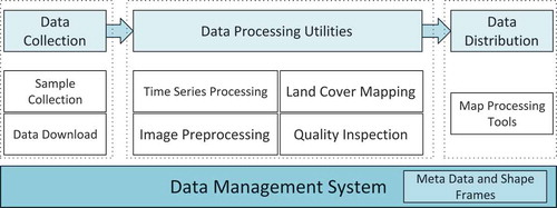
Three processes, data collection, data processing and data distribution, are indispensable for a global land cover mapping programme. Large volumes of data need to be collected and processed, and there is a huge gap between the demand for massive data processing and the available human power. Dedicated software toolkits need to be developed to provide as many as possible automations. A data management system is needed for data storage and efficient data retrieval (Figure 8). All input and output data of all processes should be stored and retrieved using this system. A data management system acts as a platform for all other software tools. Meta data and shape frames of satellite images should be collected and stored independently. This information is used for efficient data retrieval and as auxiliary sources for data processing and data analysis. The data management system should be designed scalable for progressive data accumulation. The system should provide tools for bath bulk data transfer and bulk data backup.

Figure 8. A data management and processing system for global scale land cover mapping.

A great number of samples and large volumes of data are needed for global land cover mapping. Batch download software tools need to be developed for some types of data. A tool in support of sample interpretation can improve sample collection efficiency and accuracy. The tool should be able to present a combination of all available information, such as pseudo-coloured images, spectral, annual precipitation time series, etc., to the interpreters. In addition, some handy tools, such as quick test of separability among different classes and spectral unmixing should be available to the image interpreters as well.

An automatic pre-processing system is needed that can handle as many pre-processing needs as possible. Atmospheric correction, cloud and cloud shadow detection, terrain correction, image re-projection, subsampling and image mosaicking are typical image processing procedures. Missing value processing and time series filtering are also typical time series processing procedures. Applying these procedures to satellite data at global scale requires a huge amount of manual labour if tools for batch processing are not available. Tools for visualized data overview and data consistency check are also essential for data quality inspection. High performance computing is required usually for supervised or unsupervised classification at the global scale. Specific software tools need to be developed based on the architecture of the high performance computing platform for feature extraction, sample organization, classifier training and computing resource allocation. Automatic image re-projection and image resampling should also be performed if multi-source data are used for land cover mapping.

A clear and concise presentation is important for land cover map distribution. Thumbnail images for quick overview, and appropriate layer structures for multi-temporal land cover maps are typical approaches. Potential users of global land cover data are often unfamiliar with remote sensing. It is desirable to provide the land cover data in a format that can be easily handled by users. The resolution and projection of land cover maps are usually identical to that of the original satellite images. The software tools should be able to automatically mosaic the maps in selected regions, and it can transform the mosaicked image into a user-specified projection and resolution. Class labels of land cover maps are often confusing for end users. It is also desirable to develop a tool to provide label explanation and label transformation for land cover maps.

At present, those desirable functionalities are scattered in different systems. It is highly desirable to have an integrated data management and processing system that can fulfil the needs as automatic as possible.

4.4. A portal supporting mappers to map anywhere in the world

A global land cover mapping portal can be built around the data management and analysis system proposed in the above section (Figure 9). The portal can bring together users and producers, specialists and laymen helpers in sample collection and processing, and turning the users to online-producers of local, regional and global land cover maps. This portal shall provide an online repository to hold all the training samples contributed by producers, crowdsourcing volunteers and other data users. Sources of the sample, the extracted spectral signatures, time series imagery, and other useful data, such as pictures taken in the field, are well described and managed. It further builds dedicated linkages to the publicly available land cover reference data websites, such as global observation for forest cover and land dynamics (GOFC-GOLD) Reference Data Portal, to enable a seamless access to those available reference data, such as GLC 2000 database, GlobCover 2005 database, System for Terrestrial Ecosystem Parameterization database, Visible Infrared Imaging Radiometer Suite database, Global Land Cover National Mapping Organizations 2008 training dataset and urban dataset from the University of Tokyo.

Figure 9. A proposed data portal for anyone to map anywhere in the world with all available resources in a local data management and analysis system and in the cyberspace.

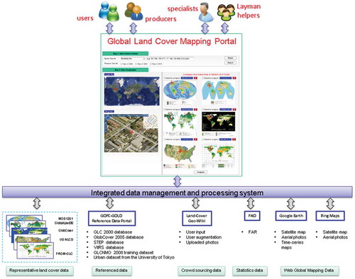
This portal will establish connections to representative land cover crowdsourcing websites, such as Land-Cover Geo-Wiki, to automatically access the local knowledge contributed by citizen scientists. Their inputs, augmentations, and uploaded photos will be available through this portal to specialists and other users. Accessing to official statistics, such as FAO Forest Resources Assessment (FRA) is necessary in this portal. This will be enabled by either maintaining the statistics data in this portal, or building dedicated data access to the corresponding statistics data systems. Web-based online Earth mapping systems, such as Google Earth and Bing Maps, will be dynamically integrated in this portal. They are valuable and independent information for users to derive land cover types.

Presenting multiple land cover data simultaneously will be available in this portal. This portal will define a specification on the land cover data access interface, and demonstrate its usefulness by enabling access to several representative land cover data, such as MOD12Q1, GlobalLand30, GlobCover, FROM-GLC, US National Land Cover Database.

To support harmonization or integration of existing land cover data, cross comparison, validation and integration functions will be developed in the portal to allow users to review, combine, improve data layers based on the available reference data, high resolution images from Google Earth, Bing Maps and local knowledge from crowdsourcing POIs and field photos.

Such a dedicated global land cover mapping portal was already initialized during the Asia-pacific GEOSS conference. It is now part of the GEO 2016 work programme. With support from China GEO, International Society for Photogrammetry and Remote Sensing and the Global Land Cover community, it is expected to be online in late 2016.

Disclosure statement

No potential conflict of interest was reported by the authors.

Additional information

Funding

This research was supported by a National Grant administrated by China Meteorological Administration [grant number 201506023].

References

- Abdullahi, S., F. Kugler, and H. Pretzsch. 2016. “Prediction of Stem Volume in Complex Temperate Forest Stands Using Tandem-X SAR Data.” Remote Sensing of Environment 174: 197–211. doi:10.1016/j.rse.2015.12.012.
- Belward, A. S., and J. O. Skoien. 2015. “Who Launched What, When and Why; Trends in Global Land-Cover Observation Capacity from Civilian Earth Observation Satellites.” ISPRS Journal of Photogrammetry and Remote Sensing 103: 115–128. doi:10.1016/j.isprsjprs.2014.03.009.
- Biradar, C. M., P. S. Thenkabail, P. Noojipady, Y. J. Li, V. Dheeravath, H. Turral, M. Velpuri, et al. 2009. “A Global Map of Rainfed Cropland Areas (GMRCA) at the End of Last Millennium Using Remote Sensing.” International Journal of Applied Earth Observation and Geoinformation 11: 114–129. doi:10.1016/j.jag.2008.11.002.
- Chen, J., J. Chen, A. P. Liao, X. Cao, L. J. Chen, X. H. Chen, C. Y. He, et al. 2015. “Global Land Cover Mapping at 30 m Resolution: A Pok-Based Operational Approach.” ISPRS Journal of Photogrammetry and Remote Sensing 103: 7–27. doi:10.1016/j.isprsjprs.2014.09.002.
- Chen, Q., P. Gong, D. Baldocchi, and Y. Q. Tian. 2007. “Estimating Basal Area and Stem Volume for Individual Trees from Lidar Data.” Photogrammetric Engineering & Remote Sensing 73 (12): 1355–1365. doi:10.14358/PERS.73.12.1355.
- Clinton, N., P. Gong, Z. Jin, B. Xu, and Z. Zhu. 2009. “Meta-Prediction of Bromus tectorum Invasion in Central Utah, United States.” Photogrammetric Engineering & Remote Sensing 75: 689–701. doi:10.14358/PERS.75.6.689.
- Clinton, N., L. Yu, and P. Gong. 2015. “Geographic Stacking: Decision Fusion to Increase Global Land Cover Map Accuracy.” ISPRS Journal of Photogrammetry and Remote Sensing 103: 57–65. doi:10.1016/j.isprsjprs.2015.02.010.
- Coppin, P., I. Jonckheere, K. Nackaerts, B. Muys, and E. Lambin. 2004. “Digital Change Detection Methods in Ecosystem Monitoring: A Review.” International Journal of Remote Sensing 25 (9): 1565–1596. doi:10.1080/0143116031000101675.
- DeFries, R. S., T. Rudel, M. Uriarte, and M. Hansen. 2010. “Deforestation Driven by Urban Population Growth and Agricultural Trade in the Twenty-First Century.” Nature Geoscience 3: 178–181. doi:10.1038/ngeo756.
- DeFries, R. S., and J. R. G. Townshend. 1994. “NDVI-Derived Land Cover Classifications at a Global Scale.” International Journal of Remote Sensing 15: 3567–3586. doi:10.1080/01431169408954345.
- Dronova, I., P. Gong, L. Wang, and L. H. Zhong. 2015. “Mapping Dynamic Cover Types in a Large Seasonally Flooded Wetland Using Extended Principal Component Analysis and Object-Based Classification.” Remote Sensing of Environment 158: 193–206. doi:10.1016/j.rse.2014.10.027.
- Eastman, R., S. G. Warren, and C. J. Hahn, 2013. “Climatic Atlas of Clouds over Land and Ocean.” Accessed November 25, 2015. http://www.atmos.washington.edu/CloudMap/index.html
- Elvidge, C. D., B. T. Tuttle, P. C. Sutton, K. E. Baugh, A. T. Howard, C. Milesi, B. Bhaduri, and R. Nemani. 2007. “Global Distribution and Density of Constructed Impervious Surfaces.” Sensors 7: 1962–1979. doi:10.3390/s7091962.
- Foley, J. A., N. Ramankutty, K. A. Brauman, E. S. Cassidy, J. S. Gerber, M. Johnston, N. D. Mueller, et al. 2011. “Solutions for a Cultivated Planet.” Nature 478: 337–342. doi:10.1038/nature10452.
- Friedl, M. A., D. K. McIver, J. C. F. Hodges, X. Y. Zhang, D. Muchoney, A. H. Strahler, C. E Woodcocka, et al. 2002. “Global Land Cover Mapping from MODIS: Algorithms and Early Results.” Remote Sensing of Environment 83: 287−302. doi:10.1016/S0034-4257(02)00078-0
- Friedl, M. A., D. Sulla-Menashe, B. Tan, A. Schneider, N. Ramankutty, A. Sibley, and X. M. Huang. 2010. “MODIS Collection 5 Global Land Cover: Algorithm Refinements and Characterization of New Datasets.” Remote Sensing of Environment 114 (1): 168–182. doi:10.1016/j.rse.2009.08.016.
- Fritz, S., L. See, I. McCallum, L. You, A. Bun, E. Moltchanova, M. Duerauer, et al. 2015. “Mapping Global Cropland and Field Size.” Global Change Biology 21: 1980–1992. doi:10.1111/gcb.12838.
- Fritz, S., L. Z. You, A. Bun, L. See, I. McCallum, C. Schill, C. Perger, J. G. Liu, M. Hansen, and M. Obersteiner. 2011. “Cropland for Sub-Saharan Africa: A Synergistic Approach Using Five Land Cover Data Sets.” Geophysical Research Letters 38 (4): L04404. doi:10.1029/2010GL046213.
- Gallant, A. L. 2015. “The Challenges of Remote Monitoring of Wetlands.” Remote Sensing 7: 10938–10950. doi:10.3390/rs70810938.
- Gao, F., E. B. de Colstoun, R. Ma, Q. H. Weng, J. G. Masek, J. Chen, Y. Z. Pan, and C. H. Song. 2012. “Mapping Impervious Surface Expansion Using Medium-Resolution Satellite Image Time Series: A Case Study in the Yangtze River Delta, China.” International Journal of Remote Sensing 33: 7609–7628. doi:10.1080/01431161.2012.700424.
- Gong, P., G. S. Biging, S. M. Lee, X. Mei, Y. Sheng, R. Pu, B. Xu, K-P. Schwarz, and M. Mostafa. 1999. “Photo-Ecometrics for Forest Inventory.” Geographic Information Sciences 5 (1): 9–14.
- Gong, P., and P. J. Howarth. 1990. “An Assessment of Some Factors Influencing Multispectral Land-Cover Classification.” Photogrammetric Engineering and Remote Sensing 56: 597–603.
- Gong, P., S. Liang, E. J. Carlton, Q. Jiang, J. Wu, L. Wang, and J. V. Remais. 2012. “Urbanisation and Health in China.” The Lancet 379: 843–852. doi:10.1016/S0140-6736(11)61878-3.
- Gong, P., J. R. Miller, and M. Spanner. 1994. “Forest Canopy Closure from Classification and Spectral Unmixing of Scene Components-Multisensor Evaluation of an Open Canopy.” IEEE Transactions on Geoscience and Remote Sensing 32 (5): 1067–1080. doi:10.1109/36.312895.
- Gong, P., J. Wang, L. Yu, Y. Zhao, Y. Zhao, L. Liang, Z. Niu, et al. 2013. “Finer Resolution Observation and Monitoring of Global Land Cover: First Mapping Results with Landsat TM and ETM+ Data.” International Journal of Remote Sensing 34: 2607–2654. doi:10.1080/01431161.2012.748992.
- Goodchild, M. 2007. “Citizens as Sensors: The World of Volunteered Geography.” GeoJournal 69: 211–221. doi:10.1007/s10708-007-9111-y.
- Herold, M., C. E. Woodcock, A. diGregorio, P. Mayaux, A. S. Belward, J. Latham, and C. C. Schmullius. 2006. “A Joint Initiative for Harmonization and Validation of Land Cover Datasets.” IEEE Transactions on Geoscience and Remote Sensing 44 (7): 1719–1727. doi:10.1109/TGRS.2006.871219.
- Hess, L. L., J. M. Melack, A. G. Affonso, C. Barbosa, M. Gastil-Buhl, and E. M. L. M. Novo. 2015. “Wetlands of the Lowland Amazon Basin: Extent, Vegetative Cover, and Dual-Season Inundated Area as Mapped with JERS-1 Synthetic Aperture Radar.” Wetlands 35: 745–756. doi:10.1007/s13157-015-0666-y.
- Hu, T. Y., J. Yang, X. C. Li, and P. Gong. 2016. “Mapping Urban Land Use by Using Landsat Images and Open Social Data.” Remote Sensing 8: 151. doi:10.3390/rs8020151.
- Huang, C., S. N. Goward, J. G. Masek, N. Thomas, Z. Zhu, and J. E. Vogelmann. 2010. “An Automated Approach for Reconstructing Recent Forest Disturbance History Using Dense Landsat Time Series Stacks.” Remote Sensing of Environment 114: 183–198. doi:10.1016/j.rse.2009.08.017.
- Hurtt, G., L. P. Chini, S. Frolking, R. A. Betts, J. Feddema, G. Fischer, J. P. Fisk, et al. 2011. “Harmonization of Land-Use Scenarios for the Period 1500–2100: 600 Years of Global Gridded Annual Land-Use Transitions, Wood Harvest, and Resulting Secondary Lands.” Climatic Change 109: 117–161. doi:10.1007/s10584-011-0153-2.
- Ji, L. Y., P. Gong, X. R. Geng, and Y. C. Zhao. 2015. “Improving the Accuracy of the Water Surface Cover Type in the 30 m FROM-GLC Product.” Remote Sensing 7: 13507–13527. doi:10.3390/rs71013507.
- Jia, K., S. Liang, N. Zhang, X. Wei, X. Gu, X. Zhao, Y. Yao, and X. Xie. 2014. “Land Cover Classification of Finer Resolution Remote Sensing Data Integrating Temporal Features from Time Series Coarser Resolution Data.” ISPRS Journal of Photogrammetry and Remote Sensing 93: 49–55. doi:10.1016/j.isprsjprs.2014.04.004.
- Jung, M., K. Henkel, M. Herold, and G. Churkina. 2006. “Exploiting Synergies of Global Land Cover Products for Carbon Cycle Modeling.” Remote Sensing of Environment 101: 534–553. doi:10.1016/j.rse.2006.01.020.
- Kennedy, R. E., Z. Yang, and W. B. Cohen. 2010. “Detecting Trends in Forest Disturbance and Recovery Using Yearly Landsat Time Series: 1. Landtrendr-Temporal Segmentation Algorithms.” Remote Sensing of Environment 114: 2897–2910. doi:10.1016/j.rse.2010.07.008.
- Li, C. C., J. Wang, L. Wang, L. Y. Hu, and P. Gong. 2014. “Comparison of Classification Algorithms and Training Sample Sizes in Urban Land Classification with Landsat Thematic Mapper Imagery.” Remote Sensing 6 (2): 964–983. doi:10.3390/rs6020964.
- Li, C. C., P. Gong, J. Wang, C. Yuan, T. Y. Hu, Q. Wang, Le Yu, et al. “A Sample Database for Seasonal Land Cover Mapping in Africa with Two Classification Schemes.” International Journal of Remote Sensing. In review.
- Li, X., P. Gong, and L. Liang. 2015. “A 30-Year (1984–2013) Record of Annual Urban Dynamics of Beijing City Derived from Landsat Data.” Remote Sensing of Environment 166: 78–90. doi:10.1016/j.rse.2015.06.007.
- Liang, L., Y. Chen, T. Hawbaker, Z. Zhu, and P. Gong. 2014. “Mapping Mountain Pine Beetle Mortality through Growth Trend Analysis of Time-Series Landsat Data.” Remote Sensing 6 (6): 5696–5716. doi:10.3390/rs6065696.
- Liu, D., and S. Cai. 2012. “A Spatial-Temporal Modeling Approach to Reconstructing Land-Cover Change Trajectories from Multi-Temporal Satellite Imagery.” Annals of the Association of American Geographers 102 (6): 1329–1347. doi:10.1080/00045608.2011.596357.
- Loveland, T. R., and A. S. Belward. 1997. “The IGBP-DIS Global 1 Km Land Cover Data Set, Discover: First Results.” International Journal of Remote Sensing 18: 3289–3295. doi:10.1080/014311697217099.
- Lunetta, R. S., J. F. Knight, J. Ediriwickrema, J. G. Lyon, and L. D. Worthy. 2006. “Land-Cover Change Detection Using Multi-Temporal MODIS NDVI Data.” Remote Sensing of Environment 105 (2): 142–154. doi:10.1016/j.rse.2006.06.018.
- Mertes, C. M., A. Schneider, D. Sulla-Menashe, A. J. Tatem, and B. Tan. 2015. “Detecting Change in Urban Areas At Continental Scales with MODIS Data.” Remote Sensing of Environment 158: 331–347. doi:10.1016/j.rse.2014.09.023
- Myneni, R. B., C. D. Keeling, C. J. Tucker, G. Asrar and R. R. Nemani. 1997. “Increased Plant Growth in the Northern Highlatitudes From 1981 to 1991.” Nature 386: 698–702. doi:10.1038/386698a0
- Niu, Z. G., H. Y. Zhang, X. W. Wang, W. B. Yao, D. M. Zhou, K. Y. Zhao, H. Zhao, et al. 2012. “Mapping Wetland Changes in China between 1978 and 2008.” Chinese Science Bulletin 57 (22): 2813–2823. doi:10.1007/s11434-012-5093-3.
- Pittman, K., M. C. Hansen, I. Becker-Reshef, P. V. Potapov, and C. O. Justice. 2010. “Estimating Global Cropland Extent with Multi-Year MODIS Data.” Remote Sensing 2 (7): 1844–1863. doi:10.3390/rs2071844.
- Radke, J., and A. Flodmark. 1999. “The Use of Spatial Decomposition for Constructing Street Center Lines.” Geographic Information Sciences 5 (1): 15–23.
- Radoux, J., C. Lamarche, E. Van Bogaert, S. Bontemps, C. Brockmann, and P. Defourny. 2014. “Automated Training Sample Extraction for Global Land Cover Mapping.” Remote Sensing 6 (5): 3965–3987. doi:10.3390/rs6053965.
- Roy, D. P., M. A. Wulder, T. R. Loveland, C. E. Woodcock, R. G. Allen, M. C. Anderson, D. Helder, et al. 2014. “Landsat-8: Science and Product Vision for Terrestrial Global Change Research.” Remote Sensing of Environment 145: 154–172. doi:10.1016/j.rse.2014.02.001.
- Schneider, A., M. A. Friedl, and D. Potere. 2010. “Mapping Global Urban Areas Using MODIS 500-M Data: New Methods and Datasets Based on ‘Urban Ecoregions’.” Remote Sensing of Environment 114: 1733–1746. doi:10.1016/j.rse.2010.03.003.
- See, L., and S. Fritz. 2006. “A Method to Compare and Improve Land Cover Datasets: Application to the GLC-2000 and MODIS Land Cover Products.” IEEE Transactions on Geoscience and Remote Sensing 44 (7): 1740–1746. doi:10.1109/TGRS.2006.874750.
- See, L., S. Fritz, C. Perger, C. Schill, I. McCallum, D. Schepaschenko, M. Duerauer, et al. 2015. “Harnessing the Power of Volunteers, the Internet and Google Earth to Collect and Validate Global Spatial Information Using Geo-Wiki.” Technological Forecasting and Social Change 98: 324–335. doi:10.1016/j.techfore.2015.03.002.
- See, L., D. Schepaschenko, M. Lesiv, I. McCallum, S. Fritz, A. Comber, C. Perger, et al. 2015. “Building a Hybrid Land Cover Map with Crowdsourcing and Geographically Weighted Regression.” ISPRS Journal of Photogrammetry and Remote Sensing 103: 48–56. doi:10.1016/j.isprsjprs.2014.06.016.
- Seto, K. C., B. Güneralp, and L. R. Hutyra. 2012. “Global Forecasts of Urban Expansion to 2030 and Direct Impacts on Biodiversity and Carbon Pools.” Proceedings of the National Academy of Sciences of the United States of America 109: 16083–16088. doi:10.1073/pnas.1211658109.
- Skidmore, A. K., N. Pettorelli, N. C. Coops, G. N. Geller, M. Hansen, R. Lucas, C. A. Mücher, et al. 2015. “Agree on Biodiversity Metrics to Track from Space.” Nature 523: 403–405. doi:10.1038/523403a
- Sleeter, B. M., T. L. Sohl, M. A. Bouchard, R. R. Reker, C. E. Soulard, W. Acevedo, G. E. Griffith, et al. 2012. “Scenarios of Land Use and Land Cover Change in the Conterminous United States: Utilizing the Special Report on Emission Scenarios at Ecoregional Scales.” Global Environmental Change – Human and Policy Dimensions 22 (4): 896–914. doi:10.1016/j.gloenvcha.2012.03.008.
- Sulla-Menashe, D., M. A. Friedl, O. N. Krankina, A. Baccini, C. E. Woodcock, A. Sibley, G. Q. Sun, V. Kharuk, and V. Elsakov. 2011. “Hierarchical Mapping of Northern Eurasian Land Cover Using MODIS Data.” Remote Sensing of Environment 115: 392–403. doi:10.1016/j.rse.2010.09.010.
- Sulla-Menashe, D., R. E. Kennedy, Z. Yang, J. Braaten, O. N. Krankina, and M. A. Friedl. 2014. “Detecting Forest Disturbance in the Pacific Northwest from MODIS Time Series Using Temporal Segmentation.” Remote Sensing of Environment 151: 114–123. doi:10.1016/j.rse.2013.07.042.
- Sun, F. D., Y. Y. Zhao, P. Gong, R. H. Ma, and Y. J. Dai. 2014. “Monitoring Dynamic Changes of Global Land Cover Types: Fluctuations of Major Lakes in China Every 8 Days during 2000–2010.” Chinese Science Bulletin 59 (2): 171–189. doi:10.1007/s11434-013-0045-0.
- Thenkabail, P. S., C. M. Biradar, P. Noojipady, V. Dheeravath, Y. Li, M. Velpuri, M. Gumma, et al. 2009. “Global Irrigated Area Map (GIAM), Derived from Remote Sensing, for the End of the Last Millennium.” International Journal of Remote Sensing 30: 3679–3733. doi:10.1080/01431160802698919.
- Thenkabail, P. S., M. A. Hanjra, V. Dheeravath, and M. Gumma. 2010. “A Holistic View of Global Croplands and Their Water Use for Ensuring Global Food Security in the 21st Century through Advanced Remote Sensing and Non-remote Sensing Approaches.” Remote Sensing 2: 211–261. doi:10.3390/rs2010211.
- United Nations. 2015. World Urbanization Prospects: The 2014 Revision. New York: Department of Economic and Social Affairs, Population Division.
- Vancutsem, C., E. Marinho, F. Kayitakire, L. See, and S. Fritz. 2013. “Harmonizing and Combining Existing Land Cover/Land Use Datasets for Cropland Area Monitoring at the African Continental Scale.” Remote Sensing 5: 19–41. doi:10.3390/rs5010019.
- Verburg, P. H., K. Neumann, and L. Nol. 2011. “Challenges in Using Land Use and Land Cover Data for Global Change Studies.” Global Change Biology 17: 974–989. doi:10.1111/gcb.2010.17.issue-2.
- Wang, J., Y. Zhao, C. Li, L. Yu, D. Liu, and P. Gong. 2015. “Mapping Global Land Cover in 2001 and 2010 with Spatial-Temporal Consistency at 250 m Resolution.” ISPRS Journal of Photogrammetry and Remote Sensing 103: 38–47. doi:10.1016/j.isprsjprs.2014.03.007.
- Wilkinson, G. G. 2005. “Results and Implications of a Study of Fifteen Years of Satellite Image Classification Experiments.” IEEE Transactions on Geoscience and Remote Sensing 43 (3): 433–440. doi:10.1109/TGRS.2004.837325.
- Xin, Q. C., P. Olofsson, Z. Zhu, B. Tan, and C. E. Woodcock. 2013. “Toward near Real-Time Monitoring of Forest Disturbance by Fusion of MODIS and Landsat Data.” Remote Sensing of Environment 135 (8): 234–247. doi:10.1016/j.rse.2013.04.002.
- Xu, G. H., Q. S. Ge, P. Gong, X. Q. Fang, B. B. Cheng, B. He, Y. Luo, and B. Xu. 2013. “Societal Response to Challenges of Global Change and Human Sustainable Development.” Chinese Science Bulletin 58 (25): 3161–3168. doi:10.1007/s11434-013-5947-3.
- Yang, J., P. Gong, R. Fu, M. Zhang, J. Chen, S. Liang, B. Xu, J. Shi, and R. Dickinson. 2013. “The Role of Satellite Remote Sensing in Climate Change Studies.” Nature Climate Change 3 (10): 875–883. doi:10.1038/nclimate1908.
- Yu, L., L. Liang, J. Wang, Y. Zhao, Q. Cheng, L. Hu, S. Liu, et al. 2014. “Meta-Discoveries from a Synthesis of Satellite-Based Land Cover Mapping Research.” International Journal of Remote Sensing 35 (13): 4573–4588. doi:10.1080/01431161.2014.930206.
- Yu, L., J. Wang, N. Clinton, Q. Xin, L. Zhong, Y. Chen, and P. Gong. 2013. “FROM-GC: 30 M Global Cropland Extent Derived through Multisource Data Integration.” International Journal of Digital Earth 6 (6): 521–533. doi:10.1080/17538947.2013.822574.
- Yu, L., J. Wang, and P. Gong. 2013. “Improving 30 m Global Land-Cover Map FROM-GLC with Time Series MODIS and Auxiliary Data Sets: A Segmentation-Based Approach.” International Journal of Remote Sensing 34 (16): 5851–5867. doi:10.1080/01431161.2013.798055.
- Yu, L., J. Wang, X. Li, C. C. Li, Y. Y. Zhao and P. Gong. 2014. “A Multi-Resolution Global Land Cover Dataset through Multisource Data Aggregation.” Science China Earth Sciences 44:1646–1660.
- Zhao, Y. Y., P. Gong, L. Yu, L. Y. Hu, X. Y. Li, C. C. Li, H. Y. Zhang, et al. 2014. “Towards A Common Validation Sample Set for Global Land-Cover Mapping.” International Journal of Remote Sensing 35: 4795–4814. doi:10.1080/01431161.2014.930202.
- Zhu, Z., and C. Woodcock. 2012. “Object-Based Cloud and Cloud Shadow Detection in Landsat Imagery.” Remote Sensing of Environment 118: 83–94. doi:10.1016/j.rse.2011.10.028.