3D geological modelling based on 2D geological map

ABSTRACT

Current methods for constructing a 3D geological model of an area require field drilling or measured section data which are often not available over large areas. 2D geological maps not only contain information on the distribution of geological strata but also provide sufficient geometric, topological and semantic information for 3D geological modelling. This paper presents a method for constructing a detail 3D model from 2D geological maps. First, a series of parallel cross sections is automatically created from the 2D geological map and the corresponding relationships of the geological objects in the cross sections are recorded. Second, a contour algorithm is used to connect these cross sections to establish a 3D geological model of the study area. The spacing of cross sections has strong impact on the result, we proposed a rule to determine the spacing of cross sections adaptively. As a case study, the method was applied to construct a 3D geological model for Xing-gang area in Chongqing city. The results of this case study suggest that the method is effective to construct a quality 3D geological model solely based on the information from a 2D geological map of the area.​​​​​

KEYWORDS:

• 2D geological map
• cross section
• 3D geological modelling
• contour algorithm

1. Introduction

Most of the existing 3D geological modelling methods depend on drilling data or measured section data observed from field. For instance, Kaufmann and Martin (2008)​​​​​ used drilling data and measured section data to build 3D geological model in coal mine. Wang, Shi, and Song (2009)​​​​​ build 3D geological Model by interpolation of drilling data. Zhu et al. (2012, 2013) build 3D solid models of sedimentary stratigraphic systems from borehole data and create geological structure fields, and property parameter fields in 3D engineering geological space depend on drilling data.​​​​​ Ming et al. (2010) used measured section data to build 3D geological model in Shunyi District’s new city zone in Beijing, China, and developed a 3D geological modelling system called the geological spatial information system.​​​​​ Wycisk et al. (2009) built a 3D geological model based on drilling data, measured section data and digital terrain model (DTM). Gong, Cheng, and Wang (2004) designed a 3D data model based on drill data and applied it to 3D geological modelling. Benito et al. (2014) designed a graphics system called the prism network and its boundary to aid 3D geological modelling based on drill data. Dong et al. (2015)​​​​​ build a 3D geological model in the inner city of Aachen, Germany, based on drilling data. GSI3D use DTM, surface geological linework and downhole borehole data to enable the geologist to construct cross sections by correlating boreholes and the outcrops to produce a geological fence diagram (http://www.gsi3d.org/research/environmentalModelling/geologicalModellingSystems.html).

Although these research and practices show that 3D geologic modelling can be successfully constructed based on drilling data and measured section data, the quality of models from these methods clearly depends on density of surveys. However, most of surveys for drilling data and measured sections tend to be clustered over areas where engineering projects tend to concentrate. Few surveys are available for other areas. It is therefore difficult to construct 3D geological models for these areas using the current methods.

Relative to the sparse drilling data and measured section data, 2D geological maps are much readily available. Mapping national and regional geological strata and structure is considered as an important task because these geological data can provide important information on some of the key resources needed for economic and social sustainable development of a country. Most countries published a series of geological maps to show the spatial distribution of geological structure and the possible locations of mineral deposits.

2D Geological maps contain the information on the distribution of geological strata and the distribution of geological structure through its depiction of strata and faults. This information provides sufficient geometric, topological and semantic information for 3D geological modelling. Hou et al. (2007) created fault plans based on the wire-frame model in accordance with analysis of the characteristics of a 2D geological map and found that the information from a geological map is useful for creating such fault planes. Wu, Xu, and Zou (2005) extracted a 3D model describing the boundary of different geological strata from a 2D geological map to assist drilling. Zanchi et al. (2009) extracted 3D information about faults and strata from a 2D geological map and used the extracted information as constraints in building 3D geological model with drilling data.

In these studies, the information from 2D geological maps only play a supporting role, drilling data or measured section data are still the major sources of data in 3D modelling. Because all of the information from geological maps usually expressed in the form of 2D, the challenge is how to extend this 2D information into 3D and construct 3D model from the extended information.

In this paper, we present a 3D geological modelling method using only the information from a 2D geological map. This method mines the information from 2D geological maps by using cross sections. Cross sections can reveal the stratum and structure within a certain depth along a certain direction from a 2D geological map (Langstaff and Morrill 1981). Cross sections are more suitable for 3D geological modelling, because they describe the 3D information of the stratum and structure along section lines.

The remainder of this paper is organized in five sections. The basic idea of using 2D geological map for 3D geological modelling is described in Section 2. Section 3 describes the detail of this modelling method. A case study and its analysis are provided in Section 4. Discussion on the effects of cross section parameters is given in Section 5. A brief conclusion is provided in Section 6.

2. Basic idea of using geological map for 3D geological modelling

The basic idea for constructing 3D geological model using information on a 2D map is to use a series of cross sections to reveal the 3D nature of geometric, topological and semantic information from 2D geological maps and then connect these cross sections by contour algorithm to establish a 3D geological model of the area.​​​​​ Cross sections in 2D geological maps provide spatial and attribute information about the stratum and geological structure along section lines (Schetselaar 1995). Serial cross sections that generated with certain spacing in study area could be considered as a discrete expression of 3D geological structure of the area. Contour algorithm can then be used to connect these serial cross sections to form a 3D representation of stratum and geological structure in the study area.

The challenge in using the above idea is how to establish the corresponding relationships of adjacent cross sections so that the geological strata shown at these cross sections are properly connected and geological structure is properly constructed in 3D. Due to the complexity of geological objects, it is very difficult to establish the corresponding relationships​​​​​ (Meyers, Skinner, and Sloan 1992; Ming et al. 2008). Cross sections are derived from the 2D geological maps, the corresponding stratum polygons, and stratum interface lines and fault lines defining the geological strata over the areas between the two adjacent cross sections must be inferred from the information in 2D geological maps. Therefore, 2D geological maps provide not only essential data sources for create cross section but also the constraints for creating the corresponding relationships between adjacent cross sections.​​​​​

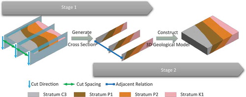
Figure 1 illustrates the stages for implementing this idea. During the first stage, a series of cross sections is generated at certain spacing cover the whole study area by parsing the 2D geological map. This stage not only provides the geometric shape and geological attribute of stratum polygons, stratum interface line and fault lines along cross sections but also creates the corresponding relationship of the polygon/polyline that described the same geological object in adjacent cross sections.​​​​​ The second stage will construct 3D geological model of study area using contour algorithm based on the generated corresponding relationships.

Figure 1. Two stages of 3D geological modelling based on 2D geological maps.

3. Methodology of 3D geological modelling based on 2D geological map

3.1. Creation of cross sections with corresponding relationships

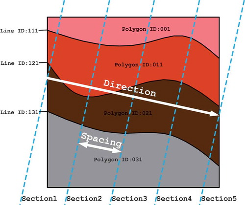
The set of cross sections should be created in parallel to each other with certain spacing (Figure 2). The general direction of the cross sections should be perpendicular to the general direction of the main geological structures in the area. Spacing should be less than the smallest geological feature to be captured in the map. A more detailed discussion of the effect of spacing on the 3D model is given in Section 5.

Figure 2. Cross section creation.

The corresponding relationships between geological features between adjacent cross sections can be determined using the polygon ID or polyline ID of the features on the 2D geological map. For example, the same stratum or fault shown on adjacent cross sections must belong to the same polygon showing this stratum or the same polyline showing the fault line on the 2D geological map. We need to assign the IDs of the polygon or polylines on the 2D geological map to the polygon or polyline on the cross sections. This allows the corresponding stratum or fault line on the adjacent cross sections to have the same ID. Consequently, the corresponding relationship of cross sections is constructed. The method for creating cross section developed by Schetselaar (1995) has been modified to allow the corresponding relationships to be constructed at the time of the creation of the cross sections.

3.1.1. Establishment of corresponding relationships for strata

First, each section line was divided into a series of connected segments according to the strata in the geological map.​​​​​ The attribute of the stratum and the ID of the polygon which intersects with the segment are assigned to the segment of the cross section, as shown in Figure 3.

Figure 3. Assignment of geological attribute value to segments of section.

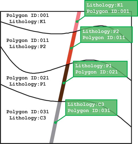
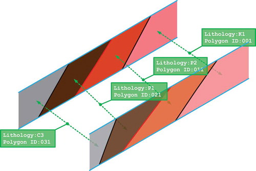
Because the ID of polygon in section comes from the stratum polygon in 2D geological map, the polygon with same ID in adjacent cross sections describes the same stratum object.​​​​​ Thereby, the corresponding relationships of stratum polygons in adjacent cross sections are established (Figure 4).

Figure 4. The corresponding relationships of stratum polygons in adjacent cross sections.

3.1.2. Establishment of corresponding relationships for strata interface and fault lines

The main geological information presented by a cross section is the spatial pattern of the stratum and fault lines. The procedure in the automatic generation of strata interface is given as follows. The procedure for fault lines is the same (Figure 5).

1. Read stratum and occurrence information from the geological maps and then conduct intersection for cross section with stratum interface to obtain the set of intersection points (P) and assign elevation values from the DEM data.​​​​​

2. Iterate the set of points (P) and create each corresponding point q as follows:

   1. Choose the stratum of point p, transform the apparent dip in occurrence obtained from the geological map to the true dip using Eqn. 2:

Figure 5. Intersection of stratum interface lines and fault lines. p0, p1, p2 are members in the set of intersection points (P), and q0, q1, q2 are the destination points.​​​​​

(2)

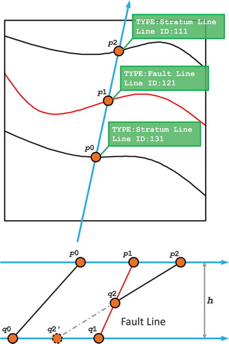
where is the direction of the cross section and is the true dip. The slope of the stratum line in the section can then be calculated using the apparent dip.

• (3) Calculate the coordinates of destination point q, the interface point of the stratum at depth h down to which the 3D geological model needs to be constructed. The length of line pq thus is .

If Line pq is fault line (p1q1 in Figure 5), the situation shown in Figure 5 will be encountered. Therefore, it is known in advance whether the fault line and the stratum line in the section intersect. If they intersect, then the stratum line is broken by the fault line – in which case the intersection point is the destination point of the stratum line and is inserted into the fault line to form a new line.

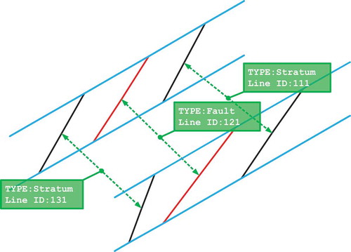
In the above process, when P is obtained, the attribute of each point of intersection in P is assigned the ID of the polyline of each stratum interface line or fault line in 2D geological maps, which intersects with the cross section. Stratum interface line or fault line pq is also assigned the same value. Thereby, the corresponding relationships of stratum interface line or fault line between adjacent cross sections are established (Figure 6).

Figure 6. The corresponding relationships of stratum interface lines or fault lines in adjacent sections.

3.1.3. Interpolation of occurrence information

The occurrence information for each segment needs to be defined for 3D construction. However, this piece of information may not be readily available due to the fact that the occurrence of the strata or fault lines is not always consistent cross the area. In addition, occurrence information is not provided for every location. Information on occurrence for each segment needs to be inferred through interpolation.

The basic assumption for inferring occurrence is as follows (Dai 2002) and shown in Figure 7: According to the definition of strike line, the upper stratum of sandstone intersects with two strata (at elevation 50 and 60 m) at strike lines I and II in the 3D perspective (Figure 7(a)), respectively.​​​​​ Angle α between line AB and the horizontal projection AC is the dip angle of the stratum. The direction of line CA is the direction of dip. The length of line BC is the difference in elevation between the two strike lines. Hence, as long as two parallel strike lines can be obtained at different heights but adjacent in the same stratum, the occurrence information of the stratum can be acquired in accordance with its elevation and horizontal distance. The planar view of this is shown in Figure 7(b).

Figure 7. Indirect interpolation of occurrence information (based on Dai (2002).​​​​​

3.2. 3D construction using contour algorithm

The basic idea underlying the contour algorithm is to create a corresponding relationship between the lines that separating different geological features on adjacent cross sections. These corresponding lines are then connected by triangulation to form the 3D model of a geologic body. During the process above, the corresponding relationships of geological objects (stratum interface lines, fault lines and stratum polygons) between adjacent cross sections have been established. All we need to do is to connect the corresponding lines of the geological objects.

The stratum interface lines, fault lines and stratum polygons on a given cross section form a particular order from one end to another end of the cross section. Thus, a cross section could be considered to be a set consisting of the stratum polygons and stratum interface lines and fault lines as its members. These members also form a particular order. Three kinds of common geological structure, basic structure, strata pinching and fault structure can be discerned based on the make-up and the order of the lines/polygons in each of adjacent cross sections.

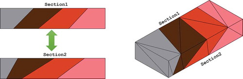
3.2.1. Modelling for basic structure

Basic structure does not involve complex geological phenomena such as strata pinching and faults. In basic structure, the adjacent cross section 1 and cross section 2 have the same set members and the same order. The fundamental idea of this model is to connect the corresponding members in two adjacent cross sections (Figure 8). The procedure is as follows:

1. All polygons in cross section are examined to find the corresponding polygon in the adjacent sections in accordance with the same attribute (polyline or polygon ID) on the geological map of the current polygon.

2. The corresponding contours of the two polygons are then joined to form the surface using the irregular triangulation network method.

Figure 8. Connection of contours to create the basic strata structure.

3.2.2. Modelling for strata pinching

Strata pinching refers to the pinching phenomena that cause the stratum on the current cross section to disappear in the next cross section due to fault or intrusion. For example, in Figure 9, it has three polygons in cross section 1 and these polygon’s stratum attributes are A, B and C, respectively. But in adjacent cross section 1, it has four polygons and their stratum attributes are A, B, D and C, respectively.

Figure 9. 2D geological maps and cross section around strata pinching.

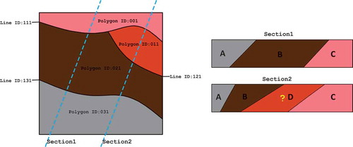
Virtual stratum polygons whose geometric structure degenerates into polyline are added in the cross section 1. The stratum polygon set in the cross section 1 could be transformed to the same structure as the cross section 2. Then, the same method as in Section 3.2.1 could be used for modelling. The procedure is as follows (Figure 10):

1. According to the particular order of the cross section 2, virtual stratum polygons whose geometric structure degenerates into polyline are added in the cross section 1. Then, the cross section 1 and 2 have the same structure.

2. The stratum polygons in the cross section 1 and 2 are connected. The connection among the non-virtual stratum polygons could be accomplished using the method in Section 3.2.1. The connection among the virtual stratum polygons could be conducted by the revised contour line method which is aimed at degenerated polygons (Ming et al. 2010). We recognize that the addition of virtual stratum may not be reflective of the actual one which disappeared between the two cross sections. However, the virtual stratum approach does allow us to connect these contours in the corrected logical order.

Figure 10. Connection of contours for strata pinching.

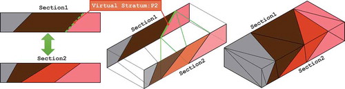
3.2.3. Modelling for fault structure

A fault divides the geologic body into several geological elements with the same stratum attribute but with spatial discrepancy (Figure 11). Therefore, connecting two polygons with same stratum attribute directly will result in error.

Figure 11. 2D geological maps and cross section around fault F.

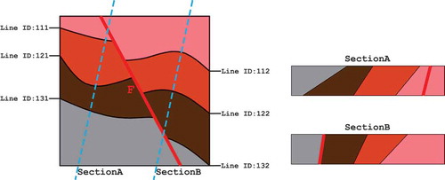
A fault is formed by dislocation of rock stratum. Therefore, by constructing the original stratum prior to formation of the fault, the strata around the fault can be modelled by simulating the dislocation of the fault. The procedure is as follows (Figure 12):

1. Create the fault surface F by connecting the fault line in cross sections A and B with the same ID;

2. At the location of cross section B, the mirror of the cross section A, A′ is created. With the method in Section 3.2.1, the cross section A and A′ are connected. The 3D geological model Solid A is created.

3. Solid A is cut by the fault surface F, Sub Solid A′ that close to the cross section A should be retained.

4. At the location of the cross section A, the mirror of the cross section B, B′ is crated. With the method in Section 3.2.1, the cross section B and B′ are connected. The 3D geological model Solid B is created.

5. Solid B is cut by the fault surface F, Sub Solid B′ that close to the cross section B should be retained.

6. Sub-Solid A′ and Sub-Solid B′ are the geological models, which is in the dislocation of fault between the cross section A and B.

Figure 12. Connection of contour around fault dislocation.

4. Case study and analysis

4.1. Study area

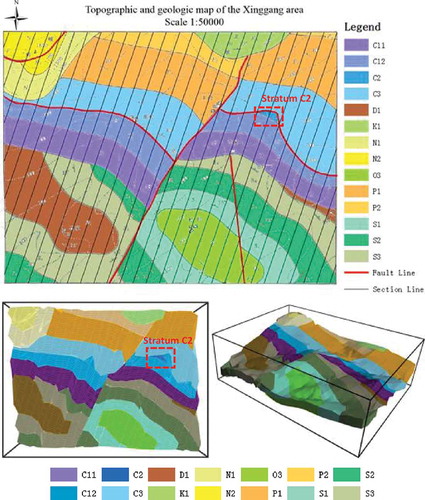
We conducted the experimental study to evaluate the method in an area of Xinggang in the Beipei district of Chongqing City. The topographic and geologic map of the Xinggang area (1:50,000) (Figure 13) is used to construct the 3D geological model of this area. A previously field observed section is used to verify the accuracy of the result.

Figure 13. Topographic and geologic map of the Xinggang area at, scale of 1:50,000. (a) 2D perspective of the Xinggang area; (b) 3D perspective of the Xinggang area

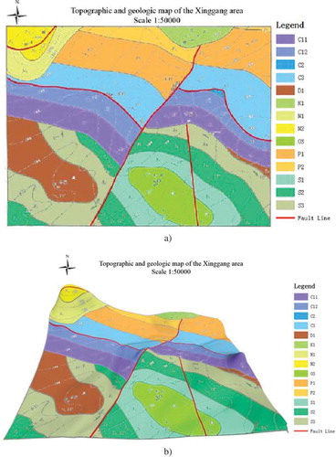
The size of Xinggang area is 960 m² and the terrain is undulating and low-lying with low elevation in the north and high elevation in the south. The strata of this area comprise Ordovician, Silurian, lower Devonian, Carboniferous, and Permian, lower Cretaceous, Miocene, and Pliocene layers. The contact relations between the lower Devonian, lower Cretaceous, Miocene and their underlying strata are angular unconformity, respectively.​​​​​

The area was stable from the late Ordovician to the early Devonian, with waterbody deepening and development of carbonate–microclastic rock formations. After the early Devonian (or late Early Devonian), Ordovician and Devonian periods, fold deformation resulted in the NNW–SSE Shijia syncline and Songcun anticline as a result of compression from SSW to NNE. In these formations, the hub of the Shijia syncline plunges to the NNW with an upright axial surface and the hub of the Songcun anticline is horizontal with axial surface inclining to SSW. After the formation of the Shijia syncline and the Songcun anticline, the study area was extended to the NEE-SWW, which resulted in a NNW–SSE F4 normal fault in the lower Ordovician to lower Devonian tectonic layers. The section of the F4 normal fault is approximately upright. The end of the early Devonian’s extrusion not only resulted in fold deformation of the upper Ordovician–lower Devonian layer but also made the study area uplift and lose the upper Devonian layer.​​​​​

At the beginning of the Early Carboniferous, the middle and northern parts of the study area started to settle and a complete Carboniferous–Permian carbonate and clastic rocks structure developed, showing a complete Transgression-Regression sedimentary series.​​​​​ After the Late Permian deposition (or the end of the late Permian), compression from the NNE to the SSW resulted in a monoclinal structure in the Permo-Carboniferous formation incline to the NE direction, and formation of F3 reverse faults in the Carboniferous–Permian layer. Compression at the end of the Late Permian uplifted the study area, resulting in the lack of the upper Cretaceous and Paleogene systems.

At the beginning of the Miocene, the northwest part of the study area began to settle, which resulted in the formation of the horizontal sedimentary of the Miocene coarse clastic and the Pliocene clastic rocks around Junling. After sedimentation of the Miocene, gravity slide structures occurred northwest of Junling, which developed an F1 normal fault between the Miocene and Pliocene layers.

4.2. Construction of a 3D geological model from the 2D geological map

Sixty-five paralleled cross sections with a spacing of 20 m along NE25° in the study area were generated automatically. From these, we were able to construct a 3D geological model of this area as shown in Figure 14.

Figure 14. Visualizations of 3D models of geologic bodies.

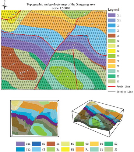
The properties of the stratum are clear and most contacts of the layers are reasonable. Fault contact F3 between the Upper Carboniferous and the Lower Carboniferous is clearly visible. Comparing the original geological map and the 3D geological model constructed, it is clear that the 3D model can generally present the geological condition of the subsurface strata in the study area.

Figure 15 is a section construct from the 3D geological model and Figure 16 is a field observed section, previously surveyed by a field geologist, over the same location. The comparison of these two sections suggests that the section from the 3D geological model closely approximates the observed one. The construct model clearly presents the structure of the NNW–SSE Songcun anticline in the Xinggang area, as well as expression of Faults F3 and F4.​​​​​ The 3D model, however, cannot capture the unexposed strata in the area as shown at D1 and C2 in Figure 16. Nevertheless, this study does indicate that our proposed method is feasible and reasonably effective approach to construct 3D geological model from a 2D geological map.

Figure 15. Section from the 3D geological model constructed.

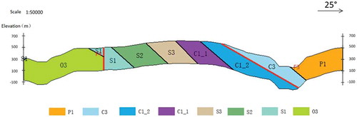
Figure 16. Measured section at the same position.

5. Discussion

The core issue of 3D geological modelling method in this paper is the use of a series of cross sections to mine the geometric, topological and semantic information from 2D geological maps. Clearly, the spacing of cross sections inevitably has strong impact on the result.​​​​​ We design an experiment to assess the impact of spacing of the cross sections. In this experiment, we use spacing 6 times larger than that used in Figure 14 to generate a series of cross section, then generate 3D geological model (Figure 17).​​​​​

Figure 17. Serial cross sections are generated by a larger spacing and then generate 3D geological model.

Clearly and naturally, larger spacing makes the 3D geological model much coarser than that from a smaller spacing. In addition, the coarse 3D model misses the smaller strata (Stratum C2 in Figure 17). The obvious solution to this problem is to decrease the spacing of cross sections. However, too many cross sections cause redundancy and it will be certainly more computational expensive.​​​​​ The other approach is to choose the spacing adaptively. Adaption can be achieved setting a spacing governing rule which states how many cross sections a geological feature must be ‘cut through’. For example, Figure 18 shows the results of using a rule of ‘at least 3 cross section per feature’. The result in Figure 18 is similar with 3D model in Figure 14.

Figure 18. The cross section after manual intervention and 3D geological model.

6. Conclusion

Due to the inherent difficulties of geological settings such as complex subsurface geometries and the lack of drilling or measured section data, we proposed a new 3D geological modelling method by using 2D geological maps, in which cross section is used as a medium. The principal advantage of this method is that the detailed 3D geological model can still be constructed with good accuracy when survey data are not available.

Disclosure statement

No potential conflict of interest was reported by the authors.​​​​​

References

- Benito, B. R., A. C. Campos, A. M. Díaz, and S. G. Cortes. 2014. “A Novel Geometric Approach for 3-D Geological Modelling.” Bulletin of Engineering Geology and the Environment 73 (2): 551–567. doi:10.1007/s10064-013-0545-9.
- Dai, J. S. 2002. Structural Geology Tutorial. Shandong: Petroleum University Press.
- Dong, M., C. Neukum, H. Hu, and R. Azzam. 2015. “Real 3D Geotechnical Modeling In Engineering Geology: A Case Study From The Inner City Of Aachen, Germany.” Bulletin Of Engineering Geology And The Environment 74 (2): 281–300. doi:10.1007/s10064-014-0640-6.
- Gong, J. Y., P. G. Cheng, and Y. D. Wang. 2004. “Three-Dimensional Modeling and Application in Geological Exploration Engineering.” Computers & Geosciences 30 (4): 391–404. doi:10.1016/j.cageo.2003.06.003.
- Hou, W. S., X. C. Wu, X. G. Liu, and G. L. Chen. 2007. “A Complex Fault Modeling Method Based on Geological Plane Map.” Rock and Soil Mechanics 28 (1): 169–172.
- Kaufmann, O., and T. Martin. 2008. “3D Geological Modelling from Boreholes, Cross-Sections and Geological Maps, Application over Former Natural Gas Storages in Coal Mines.” Computers & Geosciences 34 (3): 278–290.
- Langstaff, C. S., and D. Morrill. 1981. Geologic Cross Sections. Boston, MA: IHRDC.
- Meyers, D., S. Skinner, and K. Sloan. 1992. “Surfaces from Contours.” ACM Transactions On Graphics 11 (3): 228–258. doi:10.1145/130881.131213.
- Ming, J., M. Pan, H. G. Qu, and Z. H. Ge. 2010. “GSIS_ A 3D Geological Multi-Body Modeling System from Netty Cross-Sections with Topology.” Computers & Geosciences 36 (6): 756–767. doi:10.1016/j.cageo.2009.11.003.
- Ming, J., M. Pan, H. G. Qu, and Z. X. Wu. 2008. “Three-Dimensional Geological Multi-Body Modeling from Netlike Cross-Sections with Topology.” Chinese Journal of Geotechnical Engineering 30 (9): 1376–1382.
- Schetselaar, E. M. 1995. “Computerized Field-Data Capture and GIS Analysis for Generation of Cross Sections in 3-D Perspective Views.” Computers & Geosciences 21 (5): 687–701. doi:10.1016/0098-3004(94)00104-3.
- Wang, B. J., B. Shi, and Z. Song. 2009. “A Simple Approach to 3D Geological Modelling and Visualization.” Bulletin of Engineering Geology and the Environment 68 (4): 559–565. doi:10.1007/s10064-009-0233-y.
- Wu, Q., H. Xu, and X. K. Zou. 2005. “.An Effective Method for 3D Geological Modeling with Multi-Source Data Integration.” Computers & Geosciences 31 (1): 35–43. doi:10.1016/j.cageo.2004.09.005.
- Wycisk, P., T. Hubert, W. Gossel, and C. H. Neumann. 2009. “High-Resolution 3D Spatial Modelling of Complex Geological Structures for an Environmental Risk Assessment of Abundant Mining and Industrial Megasites.” Computers & Geosciences 35 (1): 165–182. doi:10.1016/j.cageo.2007.09.001.
- Zanchi, A., S. Francesca, Z. Stefano, S. Simone, and G. Graziano. 2009. “3D Reconstruction of Complex Geological Bodies: Examples from the Alps.” Computers & Geosciences 35 (1): 49–69. doi:10.1016/j.cageo.2007.09.003.
- Zhu, L. F., M. J. Li, C. L. Li, J. G. Shang, G. L. Chen, B. Zhang, and X. F. Wang. 2013. “Coupled Modeling between Geological Structure Fields and Property Parameter Fields in 3D Engineering Geological Space.” Engineering Geology 167: 105–116. doi:10.1016/j.enggeo.2013.10.016.
- Zhu, L. F., C. J. Zhang, M. J. Li, X. Pan, and J. Z. Sun. 2012. “Building 3D Solid Models of Sedimentary Stratigraphic Systems from Borehole Data: An Automatic Method and Case Studies.” Engineering Geology 127: 1–13. doi:10.1016/j.enggeo.2011.12.001.