Post-processing GPS-tracks in reconstructing travelled routes in a GIS-environment: network subset selection and attribute adjustment

ABSTRACT

The exact distance and routes travelled on an individual level are essential variables in determining the effectiveness of ‘soft’ transport demand management strategies. The ability to track individuals in great spatial detail by means of Location Aware Technologies such as GPS has opened avenues for gathering these data with great precision. Route reconstruction with positional data is typically done by a process referred to as map-matching; however, despite the large number of real-time map-matching algorithms developed, few studies have developed a post-processing map-matching algorithm in a Geographic Information Systems (GIS)-environment. This paper presents two GIS-based map-matching methods that predominantly use a digital road network with speed and directionality attributes for route reconstruction of raw GPS-trajectories. The methodologies were tested for a data set in which actual routes travelled were known. Both explored procedures, the ‘Connected Subset’ assignment procedure based on network subset selection and the ‘Impedance Reduction’ assignment procedure based on attribute adjustment, provide accurate results. In addition, both procedures effectively deal with commonly GPS-induced problems such as measurement gaps and positional drift.

KEYWORDS:

• Route reconstruction
• post-processing map-matching
• GPS
• Geographic Information Systems

1. Introduction

In recent years, there has been a rising interest in ‘soft’ transport demand management strategies (c.f. Cairns et al. 2008; Bonsall 2009; Brög et al. 2009; Chatterjee 2009; Stopher et al. 2009; Zhang, Stopher, and Halling 2013). The objective of these strategies, often referred to as Voluntary Travel Behaviour Change (VTBC) interventions, is typically ‘to allow people to choose to change travel behaviour rather than to expect or force reactions in response to external stimuli or pressures’ (Taylor and Ampt 2003, 171), for example, with a public information campaign aimed at informing individuals about the negative impacts of private vehicle use and highlighting public transport alternatives. Important variables in assessing the effectiveness of VTBC interventions include the exact distances and routes travelled on an individual level; information that is often difficult to acquire with traditional data collection techniques.

Since the late 1990s, Global Positioning Systems (GPS) technology and, more recently, GPS-enabled smartphones have opened avenues for accurately reconstructing the actual distances and routes travelled. Typically, this is done by assigning GPS-measurement to a digital road network by a process referred to as map-matching (Quddus, Ochieng, and Noland 2007; Hashemi and Karimi 2014). However, Dalumpines and Scott (2011, 102) note that ‘although most map-matching approaches use geometric and topological analysis, two common built-in functions in most Geographic Information Systems (GIS) packages, very limited studies have attempted to develop a post-processing map-matching algorithm in a GIS platform.’ Notwithstanding the limited deployment of GIS platforms in the development of post-processing map-matching algorithms, the inclusion of network geometry and topology is pivotal in correctly reconstructing routes as GPS is affected by measurement gaps, cold starts and signal reflection (Schuessler and Axhausen 2009b; International Transport Forum 2015). Furthermore, when adequate GIS data are available, such as detailed land use and cadastral information, a GIS offers an attractive analytical environment to integrate route reconstruction with other analyses such as activity diary reconstruction and trip purpose imputation of raw GPS-trajectories.

This paper describes two GIS-based post-processing map-matching algorithms with modest data requirements as the methods only require a topologically correct road network with speed and directionality. The first proposed algorithm selects a subset of the network, whilst the second proposed algorithm adjusts the impedance of network segments in a shortest path route assignment. A shortest path is respectively fitted through the subset of the network and the network with adjusted impedance attribute data. In addition, whilst the majority of post-processing map-matching algorithms focus solely on home to work trips by car, the applicability of the proposed map-matching algorithms for walk and bike trips is briefly explored. Especially in the context of ‘soft’ transport demand management policies in which stimulating more sustainable modes of travel is often one of the objectives, the necessity to reconstruct the bicycle and walking routes taken by individuals becomes evident.

2. Literature review

Reconstructed actual routes travelled by individuals serve transportation researchers in a number of ways, for instance, by providing input to route choice modelling exercises, estimating travel times at different times of the day and calibrating traffic models (Hashemi and Karimi 2014), as well as that the exact distance travelled is often an important variable in, for instance, evaluating the effectiveness of VTBC interventions (Bierlaire, Chen, and Newman 2013; Stopher et al. 2009; Schuessler and Axhausen 2009a). Although data on routes travelled are difficult to acquire with traditional data collection techniques, the increasing availability and ubiquity of GPS technology has enabled the collection of large amounts of high-frequency locational data. However, these raw data need to be processed in a systematic way in order to accurately identify the routes that were taken by its user, a process which is often referred to as map-matching (Quddus, Ochieng, and Noland 2007; Chen and Bierlaire 2015). Often a distinction is made between real-time map-matching algorithms and post-processing map-matching algorithms. Where real-time map-matching procedures focus on identifying the road segment on which the user is travelling and the position of the user on that road segment, post-processing map-matching algorithms aim to reconstruct the actual route travelled for an entire trip after a large number of raw GPS points has been acquired (Hashemi and Karimi 2014). In addition, in post-processing map-matching the continuity of the path route is essential, which is not a condition in real-time map-matching, allowing for more computationally intensive methods to be employed in post-processing map-matching implementations. Because real-time map-matching aims to find the actual position of the user in real-time and post-processing map-matching aims to reconstruct the actual path, ‘real-time map-matching algorithms cannot directly be used in place of post-processing map-matching algorithms as they have to resolve different challenges’ (Hashemi and Karimi 2014, 154).

The translation of raw GPS trajectories into the best estimation of a route travelled by a user is not a trivial exercise (Krumm, Gruen, and Delling 2013). This can be largely attributed to two sources of error. First, GPS faces several limitations regarding its accuracy. The environment in which the user is situated can significantly affect the accuracy of the recorded data. Whilst in open areas, GPS can be accurate up to 5 m, provided that there are at least four satellites in sight, the accuracy may decrease to 50 m as a consequence of signal blockage by, for instance, tall buildings leading to multipath signal reflection (Schuessler and Axhausen 2009b; International Transport Forum 2015). Second, the digital road network to which the GPS-measurements have to be assigned is only a digital representation of the actual world. The quality of the road network is therewith crucial in map-matching; missing or unconnected road segments can make a map-matching algorithm fail to succeed (Marchal, Hackney, and Axhausen 2005; Quddus, Ochieng, and Noland 2007). The challenge in post-processing map-matching is, therefore, to find the actual route travelled in spite of these errors (Krumm, Letchner, and Horvitz 2006).

The most basic way of map-matching works by assigning each individual GPS-measurement to the nearest road segment. The algorithm simply calculates for each GPS location the airline distance to the nearest road segment or nearest node, and the measurement is subsequently assigned to this road segment or node. The simplicity of this approach is at the same time its major limitation because neither does it account for network topology nor does it account for inaccuracies in the measurements: the nearest link is not per se the correct link (Schuessler and Axhausen 2009a). Accordingly, throughout the years, numerous map-matching techniques have been proposed that go beyond this basic method, although they have been predominantly developed in the domain of real-time map-matching (Quddus, Ochieng, and Noland 2007; Hashemi and Karimi 2014).

Whilst some of the existing map-matching techniques involve simple procedures, others are more advanced by employing, for instance, fuzzy logic, mathematical models (Bierlaire, Chen, and Newman 2013) or Bayesian Belief networks (Quddus, Noland, and Ochieng 2006; Quddus, Ochieng, and Noland 2007; Blazquez and Miranda 2014). Quddus, Ochieng, and Noland (2007) roughly categorize the methods into four types: geometric, topological, probabilistic and other advanced techniques. However, these methods are often not suitable to employ in the context of post-processing GPS-measurements because of the inherent differences in the problem that real-time and post-processing map-matching techniques are trying to address. Post-processing map-matching allows for more computational intensive procedures, but they also have to perform faster than real-time, something which has been particularly emphasized by Schuessler and Axhausen (2009a). In addition, in post-processing map-matching algorithms, the whole GPS-trajectory of a trip should be taken into account in order to ensure connectivity of the matched route (Marchal, Hackney, and Axhausen 2005).

In the past decade, several map-matching techniques have been developed and implemented in the context of post-processing raw GPS-trajectories. Early methods predominantly employed geometric procedures ranging from a simple nearest node search to curve-to-curve matching (White, Bernstein, and Kornhauser 2000). However, as Schuessler and Axhausen (2009a, 3) note, ‘the main shortcoming of all geometric procedures is that they ignore the sequence of the GPS points over time as well as the connectivity of the network links.’ Topological procedures try to avoid this shortcoming by extending the geometric approaches by taking the sequence of GPS-measurements and the connectivity of the network links into account (Velaga, Quddus, and Bristow 2009; Chung and Shalaby 2005). More statistically advanced probabilistic methods have been proposed by Marchal, Hackney, and Axhausen (2005) and Schuessler and Axhausen (2009a), who have developed algorithms where for each GPS-measurement a set of candidate paths is selected using the Multiple Hypothesis Technique. In this iterative procedure, a best candidate is selected from the set of candidate paths when the full sequence of GPS-measurements has been processed (Schuessler and Axhausen 2009a).

What all methods employed for post-processing GPS-trajectories mentioned so far have in common is their statistical or mathematical approach to solve the problem, often extended with geometrical and topological information: information that is inherent to the data model for transport networks in a GIS-environment (Papinski and Scott 2011). As Dalumpines and Scott (2011, 105) argue, this is a missed opportunity, because ‘this strength of GIS makes it an ideal platform in developing a post-processing map-matching algorithm that fully integrates network topology and attributes to match streams of GPS points to the road network.’ This also draws attention to the quality of the available data; a digital road network with minimum attributes can already be utilized for a simple map-matching solution without predefined parameters by capitalizing on this geometrical and topological information. Lastly, the fact that routes are inherently spatial manifestations on a road network also offers direct opportunities for both spatial and non-spatial data manipulation and visualization (Papinski and Scott 2011). In fact, after the map-matching procedure itself, supplementary analyses can be executed from within the GIS-environment such as activity diary reconstruction and trip purpose imputation of raw GPS-trajectories.

Although a few studies have developed a post-processing map-matching algorithm in a GIS-environment, they still adapt real-time map-matching procedures (Chung and Shalaby 2005). Dalumpines and Scott (2011) have tried to fill this void by proposing the first post-processing map-matching algorithm fully integrated into a GIS-environment. They set out to convert the stream of GPS-measurement into a polyline feature. Subsequently, they created a predefined buffer of roughly five to six times the horizontal accuracy of the measurement around the newly created polyline feature. In turn, this buffer is used to limit the network through which a shortest path is fitted between the first measurement and the last measurement in the sequence.

This shortest path predicted in 88% of the 91 routes they analysed a correct match with the actual route travelled. Whilst the buffer size with its predefined threshold distance should account for GPS inaccuracies and map inaccuracies, a limitation of the GIS-based buffer method is that the buffer size determines the success or failure of the proposed algorithm because the buffer restricts the shortest path to the network segments falling within the buffer. If the buffer size is too generous, a large number of irrelevant links can result in shorter, alternative, but incorrect, routes. If the buffer size is too small, the network might be too restrictive and completely prohibit the execution of the shortest path algorithm. In the following, therefore, two purely GIS-based map-matching procedures are described and tested that circumvent the use of a buffer and do not use other predefined parameters.

3. Proposed GIS-based map-matching algorithms

A GIS is an extremely effective tool for the incorporation of a shortest path algorithm that can effectively solve for an optimal route based on a given impedance. However, the deployment of the shortest path between two activity locations, or the first and last measurement in a sequence of GPS-measurements, is very unlikely to produce the actual route a user has travelled. In many occasions, people do not use the shortest path for reasons such as known congestion, safety and simple preference. Whereas the shortest path on its own may not be suitable for reconstructing GPS-routes, with an adjusted input the shortest path algorithm could still identify the actual route. A shortest path algorithm, for instance as developed by Dijkstra (1959), requires two sources of input besides an origin and a destination: network segments and network attributes – both of which can be manipulated. Both suggested methodologies do work, therefore, in a similar two-step approach, in which in the first step the network is either reduced or adjusted based on GPS-measurements and in the second step a shortest path between an origin and destination is fitted through the selected or adjusted network. In both cases, the GIS-extension Flowmap, specifically designed for handling spatial interaction and network data, is used for the execution of Dijkstra’s (1959) shortest path algorithm (Geertman, De Jong, and Wessels 2003).

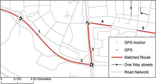
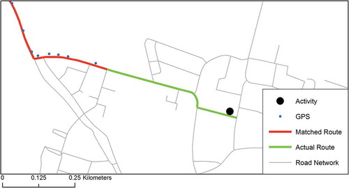
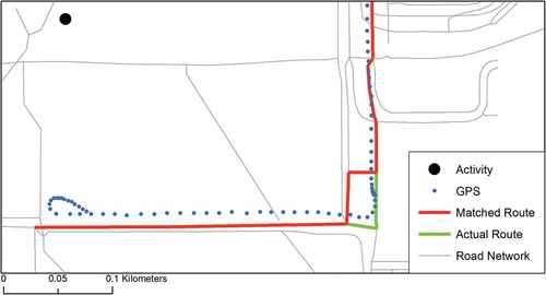
To illustrate the procedures of both proposed map-matching algorithms, a set of six GPS points has been selected, as shown in Figure 1, of a short trip by car starting in an ‘anchor’ GPS point. Using a simple nearest link search, all GPS points correctly identify parts of the actual route travelled. However, apart from the road network segments between the first measurement after the anchor and the second measurement after the anchor, substantial gaps appear between the other GPS points leading to an unconnected subnet or matched route. A relative easy way to solve this is by increasing the measurement frequency; especially for in-vehicle GPS-tracking devices, this is a viable solution. However, one should keep in mind that since the adoption of smartphones in GPS data collection, a higher measurement frequency is not always possible because of the additional impact on the already short battery life of many devices. In addition, there are several one-directional road network segments present, of which the one-directional road segments at the traffic circles seem to be important for an accurate route reconstruction. These particularities of the road network pose a simple map-matching problem in which network attribute information and directionality needs be exploited to fit a correct route.

Figure 1. Example of simple nearest link matching.

3.1. Network subset selection: connected subset

The first alternative method suggested here is the ‘Connected Subset’ assignment procedure, somewhat similar to the method described to make sense of locational data derived from cell phone records (Krygsman, Nel, and De Jong 2008) and to the real-time algorithm proposed by Miwa et al. (2012). Whereas Dalumpines and Scott (2011) use a buffer with a predefined threshold value to limit the network through which the shortest path algorithm finds a solution, the ‘Connected Subset’ assignment takes a different approach by using the full network to connect consecutive GPS-Points by a series of ‘mini’ shortest path assignments, assuming that on such a short time interval the shortest path principle always applies as it is highly unlikely that detours are made between two GPS-measurements. The combination of all these ‘mini’ shortest path assignments results in a fully connected subnetwork. In turn, a ‘maxi’ shortest path assignment is carried out through this subnetwork. The procedure involves the following steps:

1. Import a stream of GPS-measurements (representing a single trip stage) into projected coordinates.

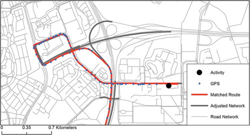
2. Connect all time adjacent GPS-measurements via the network by series of ‘mini’ shortest path assignments taking directionality and road type into account; when the mode of transport is known, a subnetwork is used for the initial matching process so that GPS-measurements that were collected when the mode of transport was a car, can only be matched to road segments that allow for travel by car. The usage of a subnetwork reduces the chance of inducing a map-matching error because of GPS inaccuracies and map inaccuracies. As shown in Figure 2, the subnet connects consecutive GPS measurement using a ‘mini’ shortest path assignment, and based on this subnet the streets between consecutive measurements can be identified. The outcome of this ‘mini’ assignment is a connected subnetwork derived from the union of the ‘mini’ shortest paths of each combination of consecutive GPS-measurements.

3. Connect the start and stop points of a trip by means of the shortest path employing the subnetwork created in the previous step. The resulting route is the shortest path generated within the extent of the connected subnetwork created in the previous step, as illustrated in Figure 3; although in this case the subnetwork is relatively straightforward, subnetworks can get quite complicated which necessitates the connection of the start and stop.

Figure 2. Creating a connected subnetwork using stepwise shortest path assignments.

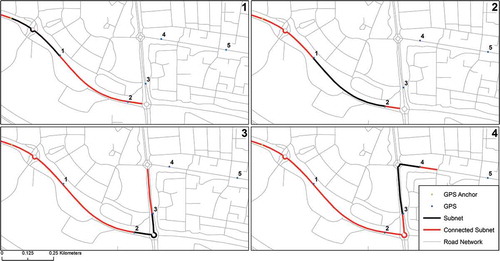
Figure 3. Correct solution with a shortest path through the connected subnetwork.

3.2. Attribute adjustment: impedance reduction

The second alternative method suggested here is the ‘Impedance Reduction’ assignment procedure, somewhat similar to the voting based algorithm proposed by Yuan et al. (2010). As opposed to the ‘Connected Subset’ assignment procedure, the ‘Impedance Reduction’ assignment procedure reduces the impedance values of road segments based on the number of nearest GPS-measurements. The result is that road segments with many hits will get a low impedance – establishing a ‘waterbed’ effect. In turn, a shortest path assignment is carried out through the full network with adjusted attributes; as opposed to the ‘Connected Subset’ assignment procedure, the shortest path is fitted only through the connected subnetwork. The procedure involves the following steps:

1. Import a stream of GPS-measurements (representing a single trip stage) into projected coordinates.

2. Connect all GPS-measurements to the digital road network by means of an attribute-based near analysis using different subsets of the full digital road network: the car network is used for car moves, the bicycle network is used for bicycle moves, the walking network is used for walk moves. This way road segments of, for instance, a highway, can only be assigned a nearest GPS-measurement by qualifying modes of transport. Again, the usage of a subnetwork reduces the chance of inducing a map-matching error because of GPS inaccuracies and map inaccuracies.

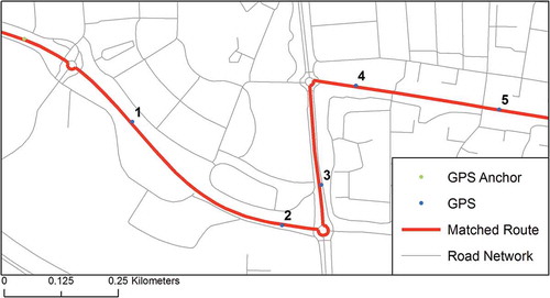
3. Count for each road segments the number (n) of nearest GPS-measurements and adjust the travel time impedance accordingly for all road segments, whereby the adjusted impedance equals the old impedance divided by 1 + n. This comes down to the same situation as presented in Figure 1, although now all ‘matched’ road segments get an impedance reduction.

4. Connect the start activity and stop activity of a trip by means of the shortest path employing the adjusted network created in the previous step. This way the shortest path assignment accounts for the network segments that were not included in the previous step of the matching procedure. The resulting route is the shortest path generated through the adjusted network in our example, resulting in the same solution as presented in Figure 3 for the ‘Connected Subset’ assignment procedure.

4. Data input and preprocessing

A GPS-data set was provided by Utrecht University, in which GPS-measurements were available from colleague ‘Maarten’ who tracked all his movements in the period from 3 December 2014 to 22 January 2015, and from 27 February 2015 to 20 March 2015. All commuter trips are done by car, but around the home bicycle and walking are also been used as alternative modes of transport. No public transport trips were recorded. In the first period, up to three different GPS-loggers were deployed simultaneously: a Garmin 72H GPS Tracking Device, an Android G20 Tablet with a MyTracks smartphone application and a Trimble data logger. In the second period, two different applications were run on the same Android device. To that end, the Trimble Data Logger was replaced with Tracklog, another smartphone application that also runs on the Android G20 Tablet.¹ Well over 200,000 unique measurements that cover over 500 km of unique road segments have been registered over the period of data collection. Table 1 gives an overview of the full data set on which both methods were tested, including devices used, the total number of measurements and the measurement frequency that was employed.

Table 1. Devices and GPS-measurements.

Device	Number of measurements	Measurement frequency (s)
Garmin 72H GPS Tracking Device	19,389	10
Android G20 Tablet (MyTracks)	188,648	1
Android G20 Tablet (Tracklog)	3,443	30
Trimble data logger	7,285	5

4.1. GPS preprocessing

In preparation, all separate track recordings per device were merged in chronological order. This way an automatic time relationship was created between the records that represent the switching off and switching on of the device, be it either on purpose or because of battery failure. After capturing the planar x-coordinates and y-coordinates, the measurements were in corroboration with Maarten transformed in a trip diary format consisting of stages, trips, stops, activities, turning points, transfer locations and travel mode, as defined in Table 2. It has to be noted that this corroboration was a necessity because the reconstruction of a trip diary based on GPS-measurements without additional information is not a trivial exercise (see for instance Schuessler and Axhausen 2009b; Montini et al. 2014; Shen and Stopher 2014) and out of scope of the current study.

Table 2. Trip diary definitions.

Movement	Description
Stage/move	A displacement with one travel mode
Trip	The sequence of stages/moves between two subsequent activity locations
Stop	A non-movement during a stage
Activity location	A location in space in which one interacts with for utilitarian or recreational purposes
Turning point	An arbitrary location that is part of a trip stage and is not an activity location, for instance, if one decides to turn around after taking a wrong turn
Transfer location	A location at the start or end of a move close to the actual activity location one is coming from or going to, for instance, a parking lot close to work or close to a supermarket or a location to switch travel mode initiating a next trip stage

The preprocessing of the GPS-measurements resulted in a trip diary including the actual mode of transport used for each trip stage. Table 3 gives an overview of all the devices with all the trip stages that are included in the analysis of both methods. Lastly, the actual routes travelled were added to a digital transport network. The digital network used was the official 2013 national road network from the Netherlands’ Cadastre, Land Registry and Mapping Agency. Since 2012 the Basisregistratie Topografie is freely available and this data set contains a detailed road network for all modes of transport. Unfortunately, speed and directionality were missing and had to be added for the relevant sections of the network, as these are a prerequisite for successfully executing a shortest path algorithm (Papinski and Scott 2011).

Table 3. Analysed trip stages.

	Car	Bike	Walk	Total
Garmin	89	31	No data	120
Android (MyTracks)	109	25	10	144
Trimble	23	4	No data	27
Android (Tracklog)	52	24	8	84
Total	273	84	18	375

4.2. Route validation

To analyse the extent to which both post-processing map-matching methods were successful, all reconstructed routes needed to be validated. ‘Validation of a map-matching algorithm is essential to derive statistics on its performance in terms of correct link identification. Very few existing map-matching algorithms provide a meaningful validation technique.’ (Quddus, Ochieng, and Noland 2007, 322) In a fashion comparable to Miwa et al. (2012), two indices were employed: the percentage of the number of road network links of the actual route that were identified correctly (% ACT) and the percentage of the number of road network links of the reconstructed route that were part of the actual route (% PRED). A score of 100% on both indices implies that the actual route travelled and the reconstructed route are identical. A score below 100% on ACT indicates that road segments of the actual route have been ‘missed’, whereas a score below 100% on PRED suggest that alternative, but incorrect, road segments are incorporated in the reconstructed route, for example, because of GPS-measurements ‘hitting’ an incorrect road segment.

5. Map-matching GPS-measurements connected subset alternative

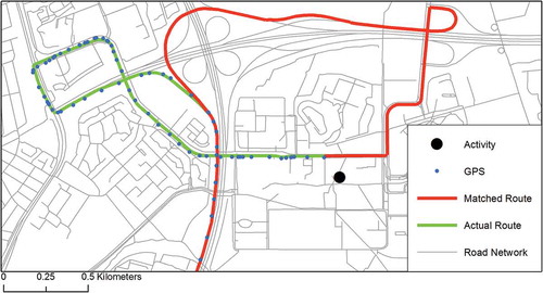
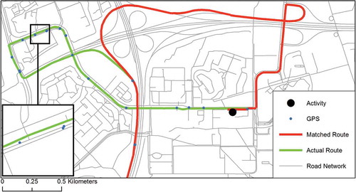
Before moving to the validation of the reconstructed trip stages for each device and each mode of travel, a graphical example of a successful execution of the procedure on a raw GPS-trajectory is shown in Figure 4. It can be seen that quite a number of side roads are included in the subnetwork that was derived in the first step of the ‘Connected Subset’ assignment. However, by execution the network subset selection through assigning ‘mini’ flows between consecutive GPS-measurements, the connectivity of the subnetwork is warranted. Moreover, by exploiting the topology and geometry stored in the GIS-network model, as well as attribute information on directionality, Figure 4 also shows that, despite the number of road segments that were included in the subnetwork and despite a noticeable gap in the raw GPS-trajectory, the trip stage is correctly fitted through the complex connected subnetwork. This suggests that there are several GPS inaccuracies or map inaccuracies present in the example, but that by executing a series of ‘mini’ assignments between consecutive measurements the correct road segments are still included in the fully connected subnetwork.

Figure 4. Example of a correct solution with a ‘maxi’ flow through the subnetwork.

A summary of the results of the validation of the analysed routes with the ‘Connected Subset’ assignment procedure is given in Table 4, and on average car moves and bike moves have high scores on both indices. Walk moves, on the other hand, did considerably less well. The fact that walking is less restricted to following the network and the low number of walk moves used in the analysis are largely responsible for these poor results. If we disregard the walk and bike moves for a moment and focus on the moves made by car, the results show index values close to 95%. However, there is a noticeable difference between the devices. The Android (MyTracks) has the highest scores. Not entirely surprising this device also had the highest measurement frequency.

Table 4. Percentages correct for the connected subnet alternative.

	Car		Bike		Walk^a
	% on ACT	% on PRED	% on ACT	% on PRED	% on ACT	% on PRED
Garmin	94.17	97.02	97.20	97.14	No data	No data
MyTracks	99.01	98.96	98.37	99.09	89.67	92.73
Trimble	89.92	98.50	100.00	100.00	No data	No data
Tracklog	92.69	93.94	96.26	97.79	88.75	100.00
Average	93.94	97.02	97.96	98.51	89.21	96.37

^aNote that only a few walking trips have been recorded.

Notwithstanding the fact that the results of the procedure generally seem to be very good, a closer examination of the problems is necessary because the large number of moves, especially in the case of the Garmin, may camouflage some mistakes in the reconstructed routes. In general, the mistakes can roughly be categorized into two categories: (1) fully GPS-induced mistakes that can only be solved by receiver technologies, and (2) procedural mistakes in which the procedure fails to correct for GPS-errors. An example of a fully GPS-induced mistake is a cold start at the start of a trip stage, as illustrated in Figure 5. Because the road segments during the cold start are not included in the subnetwork, the ‘maxi’ shortest path assignment cannot exploit those segments and, therefore, does not find the complete actual route.

Figure 5. Example of an incorrect solution with a ‘maxi’ flow through the subnetwork because of a cold start.

Other than fully GPS-induced mistakes, procedural mistakes manifest themselves as a result of measurement errors of the GPS which the procedure cannot account for. For instance, when as a consequence of inaccuracies in the GPS-measurements the size of the subnetwork increases (Figure 6): by a hit on a parallel road, the highway lane in the other direction will be incorporated in the final connected subnetwork because the ‘mini’ shortest path assignment made a successful attempt to connect the two consecutive points – although also the correct road segment is part of the mini subnetwork. Not only parallel routes can expand the subnetwork in unexpected ways, but also, as shown in Figure 7, multilevel exchanges can have this effect. The figure illustrates that the ‘GPS from’ point hits on the lower level of the multilevel exchange, whilst point ‘GPS to’ hits on the higher level of the multilevel exchange, leading to unexpected road segments incorporated in the final subnetwork. Whereas these mistakes typically do not pose a problem for the final solution, as already shown in Figure 4, the unfortunate combination of a few these mistakes may result in a subnetwork that either forces the ‘maxi’ shortest path algorithm to take an incorrect route or creates a shorter circuit that differs from the actual route travelled. An example of this is given in Figure 8: because the matched route is incorporated in the subnetwork and allows for higher travel speeds, it is incorrectly identified as the travelled route. Especially when a respondent’s trajectory ‘crosses’ itself, this problem may come into existence.

Figure 6. Example of a ‘mini’ shortest path/matched route between two consecutive GPS-measurements with matched network segments. GPS-measurements matched on different sides of the freeway; segments that will be included in the subnetwork.

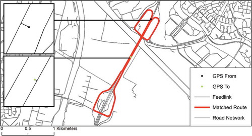
Figure 7. Example of a ‘mini’ shortest path/matched route between two consecutive GPS-measurements with matched network segments. GPS-measurements matched on different parts of a multilevel interchange; segments that will be included in the subnetwork.

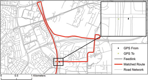
Figure 8. Example of an incorrect solution with a ‘maxi’ flow through the subnetwork.

Not only the extent of the subnetwork can affect the quality of the reconstructed routes of the ‘Connected Subset’ assignment procedure, also the shortest path assignment itself can generate an incorrect route because of inaccuracies in the digital road network. Figure 9 illustrates such a procedural mistake. The actual route has a slightly higher impedance in terms of travel time than the matched route. However, because the shorter, but incorrect, route is incorporated in the connected subnetwork because of the road segments being ‘hit’ by a GPS-measurement, the incorrect path is chosen over the actual path. Although the matched route is largely correctly reconstructed, the procedure in its current state cannot account for the errors in either measurement or road network in the situation presented. A similar situation is imaginable when the measurement frequency of the device is very low and inaccurate: the method depends on the quality of the selected subnetwork.

Figure 9. Example of an incorrect solution with a ‘maxi’ flow through the subnetwork.

6. Map-matching GPS-measurements impedance reduction algorithm

Before moving to the validation of the reconstructed trip stages for each device and each mode of travel, again a graphical example of a successful execution of the procedure is shown. Figure 10 shows a part of a raw GPS-trajectory on top of the road network supplemented with the ‘subnetwork’ of road segments that have undergone an impedance reduction in the first step of the ‘Impedance Reduction’ assignment. It can be seen that a few side roads are adjusted as well. In addition, some longer road segments are adjusted that extend well beyond the raw GPS-trajectory. However, because the impedance is only adjusted for roads that are ‘hit’ by GPS-measurements, the shortest path assignment gets drawn onto the actual route.

Figure 10. Example of adjusted road segments by GPS-hits.

The results of the validation of the analysed routes with the ‘Impedance Reduction’ assignment procedures are given in Table 5. The procedure is highly successful, as the individual scores per mode come close to a 100% score on both indices. In case of MyTracks and Tracklog, the scores for mode walk on both indices even equal 100%. It has to be noted that the walk moves are still hard to reconstruct because of the fact that they are not per se restricted to the network. This implies that for the actual routes an approximation had to be used: the closest actual path over the network. A score of 100% on both indices for mode walk, thus, means a perfect match between the reconstructed route and the approximation of the actual route taken; these results should, therefore, be interpreted with caution. If we disregard the walk and bike moves for a moment again, and turn to the moves made by car, the indices show values well over 95%. However, there is a noticeable difference between the devices; especially, the scores on both indices for Tracklog are lower than the scores for the other devices. Again, the measurement frequency seems to affect the results in case the number of hits does not adjust the impedance values enough to pull the matched route onto the actual route.

Table 5. Percentages correct for the impedance reduction alternative.

	Car		Bike		Walk^a
	% on ACT	% on PRED	% on ACT	% on PRED	% on ACT	% on PRED
Garmin	99.33	99.27	100.00	100.00	No data	No data
MyTracks	99.88	99.87	99.68	99.68	100.00	100.00
Trimble	97.34	97.72	95.51	95.51	No data	No data
Tracklog	94.26	95.62	96.20	96.86	100.00	100.00
Average	97.70	98.12	97.84	98.01	100.00	100.00

^aNote that only a few walking trips have been recorded.

Although the ‘Impedance Reduction’ algorithm seemingly performs extremely well, not all indices count to a 100%. This requires again a closer look with respect to fully GPS-induced mistakes and procedural mistakes in which the procedure fails to correct for GPS-errors. Whilst the path over the complex intersection in Figure 10 is matched effortlessly to the actual path, the matched route as shown in Figure 11 is incorrect. In this case, the travel time for the shortest route, without a correction, is just over 190 s, whereas the travel time for the actual route is just over 253 s. After the impedance reduction, the travel time of the actual routes drops to 170 s. However, the actual shortest route also gets a minor reduction in impedance as a result of GPS-hits and decreases its travel time to 164 s (Table 6).

Table 6. Supplementary table Figure 11.

	Impedance	Hits	Adjusted impedance
Matched route	190.8	4	164.6
Actual route	253.3	15	170.4

Figure 11. Example of an incorrect solution through the ‘adjusted’ network.

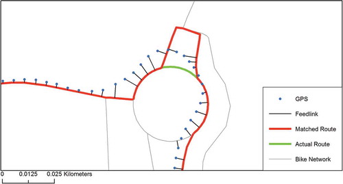
The low measurement frequency of Tracklog, thus, does not compensate for the actual shorter route. This reveals that the ‘Impedance Reduction’ procedure can lead to the same type of mistakes as the ‘Connected Subset’ assignment procedure; especially, if the measurement frequency is low. However, not only a low measurement frequency can affect the accuracy of the ‘Impedance Reduction’ assignment procedure, but also a high measurement frequency can generate an incorrect route as a consequence of inaccuracies in the GPS measurements or in the digital road network. Figure 12 illustrates such a problem: the measurements hit the road segments on different parts of the traffic circle as indicated by feed links. In turn, the matched route is being pulled off the actual route because the ‘waterbed’ effect draws the shortest path algorithm to the road segments with almost no impedance. Adjusting the impedance correction does not solve either of these problems. Where, for instance, increasing the impedance correction would solve the problem illustrated in Figure 11, it would exacerbate situations such as presented in Figure 12.

Figure 12. Example of an incorrect solution through the ‘adjusted’ subnetwork.

7. Conclusion and discussion

Important variables in assessing the effectiveness of VTBC interventions include the exact distances and routes travelled on an individual level. Whereas obtaining this information through paper-based survey instruments is extremely challenging, the increasing availability and ubiquity of locational data have, through map-matching procedures, considerably enhanced opportunities to accurately reconstruct travelled routes. This paper, therefore, sets out to describe two simple GIS-based post-processing map-matching methods. In addition, whilst post-processing map-matching algorithms have predominantly focused solely on home to work trips by car, the applicability of the proposed map-matching algorithms for walk and bike trips has been explored as well. Especially in the context of ‘soft’ transport demand management policies in which stimulating more sustainable modes of travel is often one of the objectives, the necessity to reconstruct the bicycle and walking routes taken by individuals becomes evident.

Two procedures have been proposed that support route reconstructing in a GIS-environment using preliminary a digital road network and network attributes for route reconstruction of raw GPS-trajectories without having to select predefined threshold values. In addition, the data model for transport networks in a GIS-environment allows us to effortlessly take the directionality of the road-network into account. Whereas the first proposed algorithm selects a subset of the network, the second proposed algorithm adjusts the impedance attribute data. In turn, a shortest path is fitted through the subset of the network and the network with adjusted impedance attribute data, respectively. Both explored procedures, the ‘Connected Subset’ assignment procedure based on network subset selection and the ‘Impedance Reduction’ assignment procedure based on attribute adjustment, lead to high scores on the both validation indices, especially, for trips made by car.

Notwithstanding the good results, neither procedure can account for all inaccuracies of the GPS-measurements. In the case of the ‘Connected Subset’ assignment procedure, this may surface as a consequence of a short circuit within the connected subnetwork, whilst in the ‘Impedance Reduction’ assignment procedure, the impedance correction might not compensate for shorter, but incorrect, routes as a result of the measurement frequency. It has to be noted that in case of the ‘Impedance Reduction’ procedure, the major problems only come into existence when the measurement frequency is set too low; with the second highest measurement frequency of 10 s by the Garmin, no large detour surfaced and the procedures can still be considered as robust. This signals that the deployment of the shortest path algorithm is not always applicable when the distance between two GPS-measurements becomes too large. For future studies, a possible integration with the distance and time between two consecutive points as a proxy to assess which road segments are feasible to transverse could solve some of these issues, depending on the quality and availability of a road network with detailed and accurate segment travel times. Another suggestion is to allow the initial matching to take more road segments into account by means of a distance-based ranking of nearby road segments or by turning to more probabilistic methods such as Hidden Markov model to identify candidate road segments as opposed to the shortest path algorithm.

Taken together, both methods consist of a simple, elegant and reliable procedure to deal with some of the common challenges in post-processing map-matching using a minimum of input data. This effectiveness combined with the fact that the complete operation can be executed within a GIS-environment also make it easy to automate the whole procedure using, for instance, the Python scripting language, and extend it with other types of spatial analysis on individual travel spatial behaviour; for example, when adequate GIS data are available such as detailed land use and cadastral information, a GIS offers an attractive analytical environment to integrate route reconstruction with other analyses such as activity diary reconstruction and trip purpose imputation. To conclude, it has to be noted that this paper was not per se intended to compete with existing state-of-the-art map-matching methods directly; it was rather intended to describe two relatively simple alternative methods which, by exploiting the capabilities of a GIS, can yield good results.

Disclosure statement

No potential conflict of interest was reported by the authors.

Additional information

Funding

This work was supported by the National Research Foundation (NRF), Republic of South Africa [NRF DST Innovation Scholarship] and the Graduate School of Economic and Management Sciences, Stellenbosch University, Republic of South Africa [Doctoral Scholarship]. Opinions expressed and conclusions arrived at, are those of the authors and are not necessarily to be attributed to the NRF.

Notes

1. Tracklog is a smartphone application, running on the Android and iOS operating systems, developed at Stellenbosch University, South Africa, to track individuals by means of GPS to gather travel data on an individual level to assess the effectiveness of Voluntary Travel Behaviour Change Intervention.

References

- Bierlaire, M., J. Chen, and J. Newman. 2013. “A Probabilistic Map Matching Method for Smartphone GPS Data.” Transportation Research Part C: Emerging Technologies 26: 78–98. doi:10.1016/j.trc.2012.08.001.
- Blazquez, C. A., and P. A. Miranda. 2014. “A Real Time Topological Map Matching Methodology for GPS/GIS-Based Travel Behavior Studies.” In Mobile Technologies for Activity-Travel Data Collection and Analysis, edited by S. Rasouli and H. J. P. Timmermans, 152–170. Hershey, Pennsylvania: IGI Global. doi:10.4018/978-1-4666-6170-7.ch010.
- Bonsall, P. 2009. “Do We Know Whether Personal Travel Planning Really Works?” Transport Policy 16 (6): 306–314. doi:10.1016/j.tranpol.2009.10.002.
- Brög, W., E. Erl, I. Ker, J. Ryle, and R. Wall. 2009. “Evaluation of Voluntary Travel Behaviour Change: Experiences from Three Continents.” Transport Policy 16 (6): 281–292. doi:10.1016/j.tranpol.2009.10.003.
- Cairns, S., L. Sloman, C. Newson, J. Anable, A. Kirkbridge, and P. Goodwin. 2008. “Smarter Choices: Assessing the Potential to Achieve Traffic Reductions Using ’Soft Measures’.” Transport Reviews 28 (5): 593–618. doi:10.1080/01441640801892504.
- Chatterjee, K. 2009. “A Comparative Evaluation of Large-Scale Personal Travel Planning Projects in England.” Transport Policy 16 (6): 293–305. doi:10.1016/j.tranpol.2009.10.004.
- Chen, J., and M. Bierlaire. 2015. “Probabilistic Multimodal Map Matching With Rich Smartphone Data.” Journal of Intelligent Transportation Systems 19 (2): 134–148. doi:10.1080/15472450.2013.764796.
- Chung, E.-H., and A. Shalaby. 2005. “A Trip Reconstruction Tool for GPS-Based Personal Travel Surveys.” Transportation Planning and Technology 28 (5): 381–401. doi:10.1080/03081060500322599.
- Dalumpines, R., and D. Scott. 2011. “GIS-Based Map-Matching: Development and Demonstration of a Postprocessing Map-Matching Algorithm for Transportation Research.” In Advancing Geoinformation Science for a Changing World, edited by S. Geertman, W. Reinhardt, and F. Toppen, Vol. 1, 101–120. Lecture Notes in Geoinformation and Cartography. Berlin: Springer. doi:10.1007/978-3-642-19789-5_6.
- Dijkstra, E. W. 1959. “A Note on Two Problems in Connexion with Graphs.” Numerische Mathematik 1 (1): 269–271. doi:10.1007/BF01386390.
- Geertman, S., T. De Jong, and C. Wessels. 2003. “Flowmap: A Support Tool for Strategic Network Analysis.” In Advances in Spatial Science, edited by S. Geertman and J. Stillwell, 155–175. Berlin: Springer. doi:10.1007/978-3-540-24795-1_10.
- Hashemi, M., and H. A. Karimi. 2014. “A Critical Review of Real-Time Map-Matching Algorithms : Current Issues and Future Directions.” Computers, Environment and Urban Systems 48: 153–165. doi:10.1016/j.compenvurbsys.2014.07.009.
- International Transport Forum. 2015. Big Data and Transport: Understanding and Assessing Options. Paris: OECD /ITF. http://www.internationaltransportforum.org/cpb/projects/mobility-data.html.
- Krumm, J., R. Gruen, and D. Delling. 2013. “From Destination Prediction to Route Prediction.” Journal of Location Based Services 7 (2): 98–120. doi:10.1080/17489725.2013.788228.
- Krumm, J., J. Letchner, and E. Horvitz. 2006. “Map Matching with Travel Time Constraints.” In Proceedings of the SAE 2007 World Congress, 1–7. Detroit, Michigan. doi:10.4271/2007-01-1102.
- Krygsman, S. J., H. Nel, and T. De Jong. 2008. “The Use of Cellphone Technology in Activity and Travel Data Collection in Developing Countries.” In Proceedings of the 18th International Conference on Transport Survey Methods. Annecy, France.
- Marchal, F., J. Hackney, and K. Axhausen. 2005. “Efficient Map Matching of Large Global Positioning System Data Sets: Tests on Speed-Monitoring Experiment in Zürich.” Transportation Research Record 1935 (1): 93–100. doi:10.3141/1935-11.
- Miwa, T., D. Kiuchi, T. Yamamoto, and T. Morikawa. 2012. “Development of Map Matching Algorithm for Low Frequency Probe Data.” Transportation Research Part C: Emerging Technologies 22: 132–145. doi:10.1016/j.trc.2012.01.005.
- Montini, L., N. Rieser-Schüssler, A. Horni, and K. W. Axhausen. 2014. “Trip Purpose Identification from GPS Tracks.” Transportation Research Record: Journal of the Transportation Research Board 2405: 16–23. doi:10.3141/2405-03.
- Papinski, D., and D. M. Scott. 2011. “A GIS-Based Toolkit for Route Choice Analysis.” Journal of Transport Geography 19 (3): 434–442. doi:10.1016/j.jtrangeo.2010.09.009.
- Quddus, M., R. Noland, and W. Ochieng. 2006. “A High Accuracy Fuzzy Logic Based Map Matching Algorithm for Road Transport.” Journal of Intelligent Transportation Systems: Technology, Planning, and Operations 10 (3): 103–115. doi:10.1080/15472450600793560.
- Quddus, M. A., W. Y. Ochieng, and R. B. Noland. 2007. “Current Map-Matching Algorithms for Transport Applications: State-Of-The Art and Future Research Directions.” Transportation Research Part C: Emerging Technologies 15 (5): 312–328. doi:10.1016/j.trc.2007.05.002.
- Schuessler, N., and K. W. Axhausen. 2009a. “Map-Matching of GPS Traces on High-Resolution Navigation Networks Using the Multiple Hypothesis Technique (MHT).” Working Paper 568. Institute for Transport Planning and System (IVT), ETH Zurich, Zurich.
- Schuessler, N., and K. W. Axhausen. 2009b. “Processing Raw Data from Global Positioning Systems without Additional Information.” Transportation Research Record: Journal of the Transportation Research Board 2105: 28–36. doi:10.3141/2105-04.
- Shen, L., and P. R. Stopher. 2014. “Review of GPS Travel Survey and GPS Data-Processing Methods.” Transport Reviews 34 (3): 316–334. doi:10.1080/01441647.2014.903530.
- Stopher, P. R., E. Clifford, N. Swann, and Y. Zhang. 2009. “Evaluating Voluntary Travel Behaviour Change: Suggested Guidelines and Case Studies.” Transport Policy 16 (6): 315–324. doi:10.1016/j.tranpol.2009.10.007.
- Taylor, M. A. P., and E. S. Ampt. 2003. “Travelling Smarter down Under: Policies for Voluntary Travel Behaviour Change in Australia.” Transport Policy 10 (3): 165–177. doi:10.1016/S0967-070X(03)00018-0.
- Velaga, N. R., M. A. Quddus, and A. L. Bristow. 2009. “Developing an Enhanced Weight-Based Topological Map-Matching Algorithm for Intelligent Transport Systems.” Transportation Research Part C: Emerging Technologies 17 (6): 672–683. doi:10.1016/j.trc.2009.05.008.
- White, C. E., D. Bernstein, and A. L. Kornhauser. 2000. “Some Map Matching Algorithms for Personal Navigation Assistants.” Transportation Research Part C: Emerging Technologies 8 (1–6): 91–108. doi:10.1016/S0968-090X(00)00026-7.
- Yuan, J., Y. Zheng, C. Zhang, X. Xie, and G.-Z. Sun. 2010. “An Interactive-Voting Based Map Matching Algorithm.” In Eleventh International Conference on Mobile Data Management, 43–52. IEEE. doi:10.1109/MDM.2010.14.
- Zhang, Y., P. Stopher, and B. Halling. 2013. “Evaluation of South-Australia’s Travelsmart Project: Changes in Community’s Attitudes to Travel.” Transport Policy 26: 15–22. doi:10.1016/j.tranpol.2012.06.008.