A fishnet-constrained land use mix index derived from remotely sensed data

ABSTRACT

Research works related to public health, transportation and urban planning have called for indices of land use mix (LUM) to support their spatial models. We propose a fishnet-based LUM calculation algorithm that works with the National Land Cover Database (NLCD) land cover data, a high-level product of Landsat satellite images. Comparing to the traditional LUM calculation, the fishnet structure can work at various spatial scales if aggregating to the administrative boundaries. Test results from regression models showed that our method was able to solve the scale problem identified as modifiable area unit problem that caused an unexpected positive correlation of obesity rate with LUM at the county scale. This is due to the fact that the existing methods do not limit the distance of LUM. The fishnet method provides a feasible way to calculate LUM indices across multiple scales. The NLCD data are the state-of-the art land use and land cover data for the contiguous United States. Our research provides a working example of the application of NLCD data or similar remote sensing products in public health-related research.

KEYWORDS:

• Land use mix
• NLCD
• public health
• obesity

Introduction

Land use mix (LUM), or so-called mixed land uses, defines the diversity of lands in urban areas. LUM is measured by the proximity between places of interests. It is considered to be positively associated with residents’ physical activities. In urban planning, LUM measures the degree of urban land types including commercial, residential, retail, industrial, institutional, recreational, and so on, which are intermixed in the urban landscape (Rodrigue 2013). LUM is usually calculated at the neighbourhood level from maps of land uses. It is crucial for understanding human behaviours under the influence of the built environment (Brownson et al. 2009). Therefore, it is widely used in public health research, for example, urban obesity. It is believed that through a smart-growth neighbourhood design, the built environments with better LUM could reduce the obesity rate. For example, people living in an isolated residential area rely heavily on private transportation instead of public transits or walking. In a more mixed land, people have the option to do more physical exercises through walking or biking in the shopping centres or open spaces near the neighbourhood (Manaugh and Kreider 2013).

Although there has been a consensus that LUM is associated with public health problems, the strength of such associations needs to be measured through quantitative methods. Li and Harmer (2008) found that at the block group level, each unit increase in LUM was associated with a 25% reduction in the prevalence of overweight/obesity. Rundle, Roux, and Freeman (2007) concluded that mixed land use is inversely associated with body mass index (BMI) at the census tract level in the five boroughs of New York City. Others also found that LUM was inversely associated with overweight rates (Frank, Andresen, and Schmid 2004; Mobley et al. 2006; Rundle et al. 2009). In contrast, Rutt and Coleman (2005) showed with their data that living in areas with more mixed land use was associated with higher BMI values. There are some other findings showing no statistically significant association between LUM and BMI in their case studies (e.g. Ewing, Brownson, and Berrigan 2006; Kelly-Schwartz et al. 2004). Christian et al. (2011) maintained that the relationships between different computations of LUM and walking scores varied. These contradictory findings have raised our interests in exploring the land use data for possible explanations of the inconsistency. It was pointed out that the scale used for analysis might be one of the reasons behind the issue (Brownson et al. 2009; Duncan et al. 2010). ‘Mix’ is analogous to the roughness of a surface, in which case if the observer is closer to a smooth surface, the surface could appear rough. The mixed land use usually refers to the mixture of lands at the walkable distance, for example, a maximum distance of 1–5 km. Therefore, calculation of LUM is rather a local analysis than those defined by arbitrarily selected geographic units (e.g. county polygons). However, LUM indices were usually calculated on a variety of administrative boundaries (e.g. census tract, county), ignoring the importance of spatial adjacency of the lands. In an extreme case, if the boundary of the United States was used to calculate an LUM index, without a distance to constrain it, one is literately mixing a golf course at the east coast with a residential area at the west coast. However, there is no any effort to develop a spatial computation strategy for deriving LUM indices. We argue if the distance to calculate LUM is beyond a reasonable distance, disparate conclusions might draw from statistical analyses.

On the other hand, although public health problems are of the nation-wide concern, there have been few efforts of calculating LUM at the scope of the entire United States (Song, Popkin, and Gordon-Larsen 2013; GeoDa Center 2017). There are two major technical challenges: first, it is difficult to obtain timely coverage of nation land use data by satellite images at a reasonable spatial resolution (e.g. 30 m) considering the interference of cloud cover and image processing cost; second, aggregation of the fine resolution land use data to LUM may cause the modifiable area unit problem (MAUP – Heywood, Cornelius, and Carver. 1988; Openshaw and Taylor 1979). The present research intends to solve these two problems. The National Land Cover Database (NLCD) product provided by the Multi-Resolution Land Characteristics Consortium (Homer, Fry, and Barnes 2012) is an ideal data source for land use classification at the national level. NLCD data sets were derived from Landsat satellite images and other ancillary data sets (http://www.mrlc.gov/about.php) and updated every 5 years. We will test whether the LUM can be computed from the NLCD data. Secondly, we develop a fishnet-based calculator for deriving LUM to replace the previous non-spatial methods. At last, we test the newly constructed LUM index in a regression model with obesity. We found the LUM index calculated from the traditional methods had led to an unexpected positive correlation with the obesity data at the county level. We suspect it was caused by the inappropriate spatial aggregation of the land use map to LUM, which is defined as the scale problem in MAUP (Ian, Cornelius, and Carver 1988). Our hypothesis is our new method will reduce the scale effect. And the new LUM index will be useful to model the nation-wide obesity problem.

Methodology of LUM

Approaches to calculating LUM indices can be summarized into the three categories: accessibility, intensity and distribution pattern. Accessibility is the measure to which extent the mixed land functions can be reached by the residents. Intensity is the magnitude of mixed land uses present in an area. Distribution pattern is how different types of land uses are organized in a region (Song and Rodriguez 2004).

Approaches to LUM calculation

Accessibility

Nearest neighbour distance and gravity decay distance are the two commonly used indicators of the accessibility-based LUM measurement. The nearest neighbour distance measures either the Euclidean distance or transportation network distance between residential lands and their nearest non-residential lands. The problem of this method is it only selects the nearest neighbour to calculate LUM while ignoring other lands around the residential area. The gravity model improved the nearest neighbour model by using the distance-weighted average of the distances between the residential area and its surrounding areas to calculate accessibility.

Intensity

The intensity can be measured by two methods. The number of non-residential functions around a neighbourhood is an intensity-based LUM measure. Besides, the proportions of different types of land use within a user-defined neighbourhood are a dimensionless representation of LUM. These two measurements can be obtained from the land use data. However, the intensity can be biased when there exists a large patch of non-residential land. For example, if there is a large lake in the neighbourhood, the intensity measure will not make much sense.

Distribution pattern

Song and Rodriguez (2004) defined the three aspects of LUM measured from the distribution pattern of lands: evenness, exposure and clustering. Evenness measures the balance of the land use types in a neighbourhood. Exposure measures the interaction between residential and non-residential lands (Massey and Denton 1988). Clustering considers the spatial pattern of land uses by looking at the strength of spatial clustering of a certain land type in a neighbourhood. All the indices could be associated with one of the aspects of LUM. Among them, entropy and dissimilarity are the two indices mostly used in public health-related research and supported by remote sensing data. Therefore, we will use the distribution pattern indices for LUM calculation.

LUM indices

Entropy

An entropy index measures how well the lands within a given region (e.g. a census tract or a certain distance network buffer) are divided evenly and mixed. The ideal LUM defined by entropy is the area evenly divided into the land use types. In other words, if all the land use types in an area occupy the same percentage of area, the entropy index will be a maximum (Krizek 2003). The definition of entropy was improved in the later works by Frank et al. (2005, 2006). For example, the following equation calculates the entropy index of LUM by the three-type LUM scenario in Frank et al. (2005):

(1)

where a = total area of land for all three land uses: commercial (b₁), residential (b₂) and office (b₃); n₃ = 2 or 3 depending on the number of different land uses present. If n₃ = 1 or 0, the LUM value is assigned with 0. Later, Frank et al. (2006) expanded the three-type equation to the six-type equation for LUM:

(2)

where A = (b₁/a) ln(b₁/a) + (b₂/a) ln(b₂/a) + (b₃/a) ln(b₃/a) + (b₄/a) ln(b₄/a) + (b₅/a) ln(b₅/a) + (b₆/a) ln(b₆/a); a = total square feet of land for all six land uses: single-family residential (b₁), multi-family residential (b₂), retail (b₃), office (b₄), education (b₅), entertainment (b₆); N = number of types of land use existing in the area. One advantage of entropy is it honours the diversity and balance of the land use types within a specific area. A problem, however, was raised by Krizek (2003) that an area with 10% residential land and 90% commercial land would have the same entropy value as an area with 90% residential land and 10% commercial land. Obviously, from the public health point of view, these two areas should be scored differently.

Dissimilarity

Cervero and Kockelman (1997) defined dissimilarity as ‘the mean point accumulation for a tract where each developed hectare is evaluated on the dissimilarity from surrounding hectares’. According to Cervero (1988), the equation of a dissimilarity index is

(3)

where K = number of actively developed hectares in tract; X_ik = 1 if central active hectares land use type differs from a neighbouring one (X_ik = 0 otherwise). DI is between 0 and 1 (Kockelman 1996). The advantage of dissimilarity is that the spatial adjacency or connectivity is involved in the calculation. One drawback of this definition is it only measures whether adjoining squares are different from the central square. It does not consider the diversity of the land types in the neighbourhood (Hess, Moudon, and Logsdon 2000).

Concentration

Another measure of LUM is the ‘index of concentration’ (Bendavid-Val 1991):

(4)

where %DA_j is the percentages of the developed area and %Attribute_j is the single attribute type within each sub-zone j. This measurement requires a division of a single zone into several sub-zones which is not practical at the neighbourhood level.

Fishnet-based method for NLCD data

The aforementioned methods have been used to calculate LUM indices of a city or a county. The basic geographic units were either a census tract or a block group. In these cases, the LUM calculation was approximately within walking distances (Frank et al. 2010, Riva et al. 2008). However, because our goal is to calculate the nationwide LUM index, the basic unit cannot be set as a census tract or anything lower. Other than the high computation cost, the data availability, such as obesity data, is also a concern in a low-level geographic unit. Given that most public health data are usually aggregated to county boundaries before releasing to the public, computation of LUM at the county boundary is important.

If the entropy index Equation (1) by Frank et al. (2005) is used to a county, the distance between the lands are usually beyond walkable. Then mixing the lands will not carry any meaning to walkability or physical activities concerned by public health studies. Therefore, there should be a control of the calculation distance imposed on the equation. The fishnet structure implemented by the GIS can be such a solution.

One other concern about the previously defined land use indices is they were not designated for public health research using the NLCD data. Although theoretically, residential, commercial, industrial, recreational and institutional are typically used in LUM measures, not all of these land use types provide walkable destinations for residents. If LUM is not appropriately defined, the LUM index might be misinterpreted and may conceal the relationship between LUM and residence’s behavioural outcomes (Glanz, Rimer, and Viswanath 2008). Moreover, the LUM definition should be situated on residential land use, because the physical activities are assumed to occur near where people live. If an area has no residential land use, the LUM index should be assigned as zero so it does generate factors for physical activities. With those concerns about the previously used LUM calculation, we propose a new method that extends the existing entropy method by Frank et al. (2005) by a GIS-based spatial tessellation (fishnet) method and redefine the equations to use the NLCD land use data.

Data and the new fishnet-based LUM index calculation

Reprocessing the NCLD data

For the land use data, we refer to the NLCD published by the Multi-Resolution Land Characteristics Consortium (MRLC). MRLC is a joint effort of several federal agencies led by the US Geological Survey to put together land cover information at the national scale (Homer, Fry, and Barnes 2012). NLCD is derived from Landsat satellite images and other ancillary data sets (http://www.mrlc.gov/about.php).

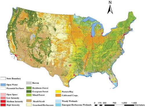
The map in Figure 1 is created from the NLCD 2006 data set, which classifies lands into multilevel land cover and land use (LULC). The classification scheme was modified from the Anderson’s LULC classification system (Anderson 1976). The classes are coded with two digits. The first digit marks the level I class and the second is for level II. We focused on the level II classes under the category of ‘developed’ class, including open space, low-intensity, medium-intensity and high-intensity built-up areas. Both low-intensity and medium-intensity classes are likely to be residential areas. Therefore, they fall into the residential land class. The high-intensity class is more likely to be the commercial land use. It is thus treated as the commercial land use. We shall acknowledge that in some circumstances, the industrial lands would also be classified as ‘high intensity’ in NLCD data. Therefore, there might be some commission errors in the commercial land use class. Our method, however, is resistant to those commission errors because of the utility of fishnets to define walkable distance. In other words, those industrial lands are usually placed at remote areas from residents due to the factors of pollution and noise. In our calculation, such lands will be excluded automatically by the fishnet distance threshold. Other land cover types were marked as ‘no data’ to exclude them from LUM calculation.

Figure 1. Land use patterns in the contiguous United States. Data are obtained from NLCD 2006.

Colours were defined according to the NLCD 2006 legend.

The NLCD data have been reported to be reasonably accurate according to the report by the GeoDa Center of Arizona State University on their website (GeoDa Center 2017). Wickham et al. (2013) also showed the 2006 NLCD data had sufficient accuracy. Especially, both the user’s accuracy and producer’s accuracy of the four classes we used were quite high. To further validate the land use data derived from the NLCD data, we ran several verifications using data from other sources. For example, we checked the land use maps from the Twin Cities Metropolitan Council of Minnesota (Forsyth et al. 2007). The maps include land use data spanning 1970–2011 at 5-year intervals in a coincidental timing with the NLCD data. We verified that the NLCD data were accurate compared to the local land use maps.

Fishnet-based entropy method

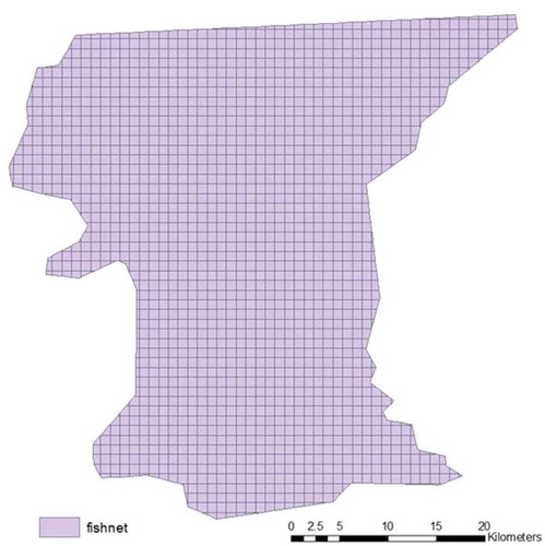
Fishnet is a GIS technique to create a mesh of rectangles, which tessellates the study area into uniform units. Each unit is independently computed by Equation (5). It is similar to a raster data tessellation except the units are defined in the ‘vector’ format for the ease of spatial operations such as clipping and zonal statistics. We created the 1-km square fishnet grids covering each county. Figure 2 shows the fishnet cells created in the state of Louisiana boundary. The LUM values are calculated at each cell. As noted before, if there is no residential area within the range of the 1-km cell, the LUM value for that cell will be 0. The county will then have its LUM value assigned from averaging all the fishnet cells within its boundary. Although all the previously used LUM equations are applicable, in this paper, we only test the equation of entropy index (EI) by Frank et al. (2005) to discuss our new method:

(5)

Figure 2. Fishnet in East Baton Rouge County, Louisiana.

where p_ij is the proportion of land use i in area j, and n_j is the number of land uses in area j. Because we only have three valid land use classes, n can be assigned as 1, 2 or 3, depending on the number of land use types in each fishnet unit. Although choices of the denominator might be arbitrary, such as the one by Hajna et al. (2014), our test showed the impact of the denominator is minimal. EI from Equation (5) is a continuous floating point number ranging from 0 to 1, where 0 means there is no LUM in the area and 1 indicates an ideal condition of LUM for public health models. In this way, EI values are assigned to each fishnet cell. The county LUM value is an average of the EI by the fishnet cells. For comparison purposes, we also calculated county EI by directly applying the equation at the county boundaries.

The fishnet-based algorithm was implemented in the ArcGIS version 10.1 environment supported by ESRI ArcObjects and Microsoft Visual Studio 2010. To handle the large volume of data with better efficiency, we clipped the NLCD data by states and run the algorithm separately in virtual machines of a parallel computing system. The average processing time for each state is 15 min on an Intel core-2 1.6 GHz desktop computer with 6 GB memory. Without parallel computing, it would take about 3 days to complete the computation for the entire United States.

Results and discussion

Spatial pattern of LUM

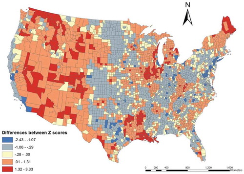
The standardized Z-score (with a zero mean and standard deviation of 1) of the values from the new method (fishnet based) and the traditional method (county boundary based) are compared as shown in Figure 3. Dark colours are higher Z-scores, that is, entropy values above the national mean. Notably, the LUM is higher in the eastern areas than the western areas in the map generated by the traditional (non-fishnet) method. However, the spatial patterns of LUM are very different in the map generated by the fishnet method. For example, the states of Washington and California have higher LUM among most areas. The states in the mountain area have high LUM. The states in the centre zones have low-to-medium LUM values. Both maps agree on the high LUM values of the Atlantic area regardless the calculation algorithm. To make the difference between the two methods more outstanding, we created the county value difference map in Figure 4. Warm colours on the map indicate the LUM value from our method is greater than the traditional method, and vice versa. Most counties in the western United States have greater LUM values resulted from adopting the fishnet algorithm, while it is opposite in the east. The discrepancy of the results suggests the fundamental change in statistics when using the GIS-based computation to replace pure statistical equations. It is in a similar spirit of the argument in MAUP that a change in the scale might totally reverse the statistical models (Ian, Cornelius, and Carver 1988). Our method cannot completely solve the MAUP scale problem because we still have to use aggregation on the fishnet cells to arbitrary units such as counties. However, our method at least avoids the misinterference on the land use data at different scales.

Figure 3. Entropy index standardized Z-score at county level by (a) original method and (b) fishnet method.

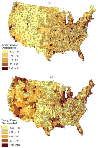
Figure 4. Differences in land use mix (LUM) index at county level by comparing the fishnet method with the traditional method.

Effects on regression models

Our new method uses the fishnet grids to confine the scale of computation for LUM. By reasoning, it would be a better solution than those disregarding the scale of the arbitrary geographic units. The unit of the fishnet is chosen as 1 km – a reasonable range for physical activities such as walking or biking (Yamada et al. 2012). The selection of the 1-km distance as the grid size is backed up by the previous local studies such as in Rundle et al. (2009). Defining the walkable distance in an LUM calculation is important because otherwise the lands will be mixed at the distance far beyond walkability. For example, the average size of the counties is 2502 km² in the conterminous United States. The maximum Euclidean distance of two points in an average-size county, if assuming a perfect circular shape, would be 56 km (the diameter of the circle). This distance is even beyond a regular driving distance. Mixing the lands that are 56 km apart does not help improve the built environment related to public health.

Our modification to the entropy equation by Frank et al. (2005) is justifiable with the NLCD data. We argue the LUM calculation should be focused on the residential lands. Without including people (residence) in the equation by Frank et al. (2005), the LUM will deviate from its primary purpose. This argument can be fulfilled by our fishnet method because of the spatial tessellation. In other words, by dividing the counties into fishnets, we can exclude the fishnet cells that do not have any residential areas from aggregation in the counties.

We calculated the LUM index also by Equation (5) without using the fishnet. Then we tested the correlation with the county-level obesity rate of both LUM indices. The county-level obesity rate data were obtained from the CDC’s website on Diabetes Data & Trends (https://www.cdc.gov/diabetes/data/countydata/countydataindicators.html). We built a regression model by including three more variables – population density, race heterogeneity and poverty. The regression equation is

(6)

where obesity rate (Obesity) is the dependent variable, β₀, β₁, β₂ and β₃ are the regression coefficients, whereas ɛ is the random error. Population density (PopDen) is defined by the population per square kilometre. Race heterogeneity (RaceHetero) reflects the racial composition which is measured as 1– ∑pi², where pi is the proportion of the population in a given group (Xu and Wang 2015; Sampson 1989). Poverty rate (Poverty) rate is the per cent of people of all ages in poverty, which was downloaded at the website of the US population Census (http://www.census.gov/did/www/saipe/data/statecounty/data/index.html). The regression using the LUM from the traditional method resulted in a significant and positive coefficient, which suggested larger LUM values were associated with more obesity. This is unaccepted with the LUM theory (Dur, Yigitcanlar, and Bunker 2014; Manaugh and Kreider 2013; Song, Merlin, and Rodriguez 2013; Ratner and Goetz 2013) and needs to be fixed. We hypothesize two possible causes of this problem. First, the aggregation of land use and obesity data in the county boundaries might have the scale MAUP problem (Openshaw and Taylor 1979). However, as shown in Openshaw and Taylor (1979), the change in the zoning scale only affected the spread of the correlation coefficient but rarely change the sign of it. The second hypothesis is that without using distance constraint, the LUM index calculated from Equation (5) is wrong. And if we apply the fishnets on the equation, the LUM index can be rectified.

To compare the LUM from the traditional method and fishnet method, we tested three regression models: the first model uses the independent variables excluding the LUM variable; the second model adds the LUM index from Equation (5) but without the fishnets; the third model replaces the LUM variable by the fishnet-based LUM. These three models will show the differences in the explanatory power between the original and the fishnet LUM methods. The results are shown in Table 1. The population density, race heterogeneity and the poverty rate variables have the expected effect in all the models. Also, the changes in t-score and R² shown at the bottom of the table are very telling. The LUM from the traditional method is positively associated with the obesity rate. It turned out that after we employed the new LUM index calculated from the fishnet method, the coefficient became negative as expected in the theory. Therefore, we conclude at the county scale, LUM cannot be directly computed on the county boundaries using the equations by previous research (Frank et al. 2006; Frank et al. 2005). Adding fishnets as spatial constraints on the equations is the solution to the LUM from NLCD data at the nationwide coverage.

Table 1. Ordinary least square models on obesity rate at the county level.

	No mix variable		Original		Fishnet
Variables	β	t	β	t	β	t
Constant	23.26	154.211	22.78	125.78	23.70	125.17
Population density	−0.0003 ***	−6.11	−0.0003 ***	−7.55	−0.0002 **	−5.09
Race heterogeneity	−2.42 ***	−7.74	−2.84 ***	−878	−2.21 ***	−7.00
Poverty rate	0.31 ***	32.39	0.33 ***	32.39	0.305	30.69
Original (Z)			1.81 ***	4.82
Fishnet (Z)					−1.16 *	−3.81
Adjusted R^2	0.270		0.276		0.273

***p ≤ 0.001, **p ≤ 0.01, *p ≤ 0.05.

Sensitivity of the fishnet size

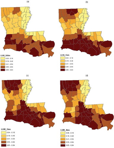
In our experiment, the unit of the fishnet was chosen as 1 km by 1 km squares according to previous knowledge about LUM (Yamada et al. 2012). However, this is still an arbitrary number, with which the uncertainty associated must be tested to make sure the model was not severely biased by arbitrarity. We tested four different fishnet sizes: 500 m, 1 km, 2 km and 4 km. Because of the data volume, we use the state of Louisiana for testing the model sensitivity. Figure 5 shows the LUM indices created by different fishnet sizes. The 2-km and 4-km fishnets produced very similar patterns, suggesting there is no major change between these two sizes. The 500-m fishnet created LUM values smaller than those from the 1-km fishnet. However, we suspect that 500-m cell size might be too small as the maximum walkable distance. The land use index – entropy is not sensitive to the fishnet cell size. Overall, we believe 1 km is a reasonable setting for LUM calculation.

Figure 5. LUM index from different sizes of fishnet: (a) 500 m; (b) 1 km; (c) 2 km; and (d) 4 km.

Conclusion

We presented the procedure and results of using the 1-km fishnet structure to measure LUM at the national scale from remotely sensed data. We were able to create a county LUM map from the NLCD by a fishnet-based entropy algorithm in the GIS. A regression analysis verified that by using the fishnets to constrain the entropy computation the LUM variable had a negative association with obesity. It is backed up by the ideology of smart urban growth with mixed use. Our research showed a workable solution for deriving the LUM variable at the county level with nationwide coverage can be derived from the NLCD data set. With the timely update of the NLCD data (currently 2010, and 2015 in the near future), we will be able to relate LUM dynamics to longitudinal nationwide public health problems.

Disclosure statement

No potential conflict of interest was reported by the authors.

Additional information

Funding

This work was supported by the Summer Research Awards and Fellowships Program of the University of Toledo [3893].

References

- Anderson, J. R. 1976. A Land Use and Land Cover Classification System for Use with Remote Sensor Data. Vol. 964. Washington, DC: US Government Printing Office.
- Bendavid-Val, A. 1991. Regional and Local Economic Analysis for Practitioners. 4th ed. Westport, CT: Praeger.
- Brownson, R. C., C. M. Hoehner, K. Day, A. Forsyth, and J. F. Sallis. 2009. “Measuring the Built Environment for Physical Activity: State of the Science.” American Journal of Preventive Medicine 36 (4): SS99–123. doi:10.1016/j.amepre.2009.01.005.
- Cervero, R. 1988. “Land-Use Mixing and Suburban Mobility.” Transportation Quarterly 42 (3): 429–446.
- Cervero, R., and K. Kockelman. 1997. “Travel Demand and the 3ds: Density, Diversity, and Design.” Transportation Research Part D: Transport and Environment 2 (3): 199–219. doi:10.1016/S1361-9209(97)00009-6.
- Christian, H. E., F. C. Bull, N. J. Middleton, M. W. Knuiman, M. L. Divitini, P. Hooper, A. Amarasinghe, and B. Giles-Corti. 2011. “How Important Is the Land Use Mix Measure in Understanding Walking Behaviour? Results from the RESIDE Study.” The International Journal of Behavioral Nutrition and Physical Activity 8 (1): 55. doi:10.1186/1479-5868-8-55.
- Duncan, M. J., E. Winkler, T. Sugiyama, E. Cerin, L. duToit, E. Leslie, and N. Owen. 2010. “Relationships of Land Use Mix with Walking for Transport: Do Land Uses and Geographical Scale Matter?” Journal of Urban Health 87 (5): 782–795. doi:10.1007/s11524-010-9488-7.
- Dur, F., T. Yigitcanlar, and J. Bunker. 2014. “A Spatial-Indexing Model for Measuring Neighbourhood-Level Land-Use and Transport Integration.” Environment and Planning B: Planning and Design 41 (5): 792–812. doi:10.1068/b39028.
- Ewing, R., R. C. Brownson, and D. Berrigan. 2006. “Relationship between Urban Sprawl and Weight of United States Youth.” American Journal of Preventive Medicine 31 (6): 464–474. doi:10.1016/j.amepre.2006.08.020.
- Forsyth, A., L. Lytle, N. Mishra, P. Noble, and D. Van Riper. 2007. Environment, Food, +Youth: GIS Protocols. Edited by Ann Forsyth. University of Minnesota, TREC.
- Frank, L. D., M. A. Andresen, and T. L. Schmid. 2004. “Obesity Relationships with Community Design, Physical Activity, and Time Spent in Cars.” American Journal of Preventive Medicine 27 (2): 87–96. doi:10.1016/j.amepre.2004.04.011.
- Frank, L. D., J. F. Sallis, T. L. Conway, J. E. Chapman, B. E. Saelens, and W. Bachman. 2006. “Many Pathways from Land Use to Health: Associations between Neighborhood Walkability and Active Transportation, Body Mass Index, and Air Quality.” Journal of the American Planning Association 72 (1): 75–87. doi:10.1080/01944360608976725.
- Frank, L. D., J. F. Sallis, B. E. Saelens, L. Leary, K. Cain, T. L. Conway, and P. M. Hess. 2010. “The Development of a Walkability Index: Application to the Neighborhood Quality of Life Study.” British Journal of Sports Medicine 44 (13): 924–933. doi:10.1136/bjsm.2009.058701.
- Frank, L. D., T. L. Schmid, J. F. Sallis, J. Chapman, and B. E. Saelens. 2005. “Linking Objectively Measured Physical Activity with Objectively Measured Urban Form: Findings from SMARTRAQ.” American Journal of Preventive Medicine 28 (2): 117–125. doi:10.1016/j.amepre.2004.11.001.
- GeoDa Center. 2017. Land Use Mix. Chicago, IL: The University of Chicago.
- Glanz, K., B. K. Rimer, and K. Viswanath. 2008. Health Behavior and Health Education: Theory, Research, and Practice. 4th ed. San Francisco, CA: Jossey-Bass.
- Hajna, S., K. Dasgupta, L. Joseph, and N. A. Ross. 2014. “A Call for Caution and Transparency in the Calculation of Land Use Mix: Measurement Bias in the Estimation of Associations between Land Use Mix and Physical Activity.” Health & Place 29: 79–83. doi:10.1016/j.healthplace.2014.06.002.
- Hess, P. M., A. V. Moudon, and M. G. Logsdon. 2000. “Measuring Land Use Patterns for Transportation Research.” Transportation Research Record 1: 17–24.
- Homer, C. H., J. A. Fry, and C. A. Barnes. 2012. The National Land Cover Database. Sioux Falls, SD: U.S. Geological Survey.
- Ian, H. D., S. Cornelius, and S. Carver. 1988. An Introduction to Geographical Information Systems. New York: Addison Wesley Longman.
- Kelly-Schwartz, A. C., J. Stockard, S. Doyle, and M. Schlossberg. 2004. “Is Sprawl Unhealthy?: A Multilevel Analysis of the Relationship of Metropolitan Sprawl to the Health of Individuals.” Journal of Planning Education and Research 24: 184–196. doi:10.1177/0739456X04267713.
- Kockelman, K. M. 1996. “Travel Behavior as a Function of Accessibility, Land Use Mixing, and Land Use Balance: Evidence from the San Francisco Bay Area.” Master of City Planning, City and Regional Planning, University of California, Berkeley.
- Krizek, K. J. 2003. “Operationalizing Neighborhood Accessibility for Land Use - Travel Behavior Research and Regional Modeling.” Journal of Planning Education and Research 22: 270–287. doi:10.1177/0739456X02250315.
- Li, F., and P. A. Harmer. 2008. “Built Environment, Adiposity, and Physical Activity in Adults Aged 50–75.” American Journal of Preventive Medicine 35 (1): 38–46. doi:10.1016/j.amepre.2008.03.021.
- Manaugh, K., and T. Kreider. 2013. “What Is Mixed Use? Presenting an Interaction Method for Measuring Land Use Mix.” The Journal of Transport and Land Use 6 (1): 63–72.
- Massey, D. S., and N. A. Denton. 1988. “The Dimensions of Residential Segregation.” Social Forces 67 (2): 281–315. doi:10.1093/sf/67.2.281.
- Mobley, L. R., E. D. Root, E. A. Finkelstein, O. Khavjou, R. P. Farris, and J. C. Will. 2006. “Environment, Obesity, and Cardiovascular Disease Risk in Low-Income Women.” American Journal of Preventive Medicine 30 (4): 327–332. doi:10.1016/j.amepre.2005.12.001.
- Openshaw, S., and P. J. Taylor. 1979. “A Million or so Correlation Coefficients: Three Experiments on the Modifiable Areal Unit Problem.” Statistical Applications in the Spatial Sciences 21: 127–144.
- Ratner, K. A., and A. R. Goetz. 2013. “The Reshaping of Land Use and Urban Form in Denver through Transit-Oriented Development.” Cities 30: 31–46. doi:10.1016/j.cities.2012.08.007.
- Riva, M., P. Apparicio, L. Gauvin, and J.-M. Brodeur. 2008. “Establishing the Soundness of Administrative Spatial Units for Operationalising the Active Living Potential of Residential Environments: An Exemplar for Designing Optimal Zones.” International Journal of Health Geographics 7: 43. doi:10.1186/1476-072X-7-43.
- Rodrigue, J.-P. 2013. “Urban Land Use and Transportation.” In The Geography of Transport Systems, edited by J.-P. Rodrigue, C. Comtois, and B. Slack. New York: Routledge.
- Rundle, A., K. M. Neckerman, L. M. Freeman, G. S. Lovasi, M. Purciel, J. Quinn, C. Richards, N. Sircar, and C. Weiss. 2009. “Neighborhood Food Environment and Walkability Predict Obesity in New York City.” Environmental Health Perspectives 117 (3): 442–447. doi:10.1289/ehp.11590.
- Rundle, A., A. Roux, and L. M. Freeman. 2007. “The Urban Built Environment and Obesity in New York City: A Multilevel Analysis.” American Journal of Health Promotion 21: 326–334. doi:10.4278/0890-1171-21.4s.326.
- Rutt, C. D., and K. J. Coleman. 2005. “Examining the Relationships among Built Environment, Physical Activity, and Body Mass Index in El Paso, TX.” Preventive Medicine 40 (6): 831–841. doi:10.1016/j.ypmed.2004.09.035.
- Sampson, R. J. 1989. “Community Structure and Crime: Testing Social-Disorganization Theory.” American Journal of Sociology 94 (4): 774–802. doi:10.1086/229068.
- Song, Y., L. Merlin, and D. A. Rodriguez. 2013. “Comparing Measures of Urban Land Use Mix.” Computers, Environment and Urban Systems 42: 1–13. doi:10.1016/j.compenvurbsys.2013.08.001.
- Song, Y., B. Popkin, and P. Gordon-Larsen. 2013. “A National-Level Analysis of Neighborhood Form Metrics.” Landscape and Urban Planning 116: 73–85. doi:10.1016/j.landurbplan.2013.04.002.
- Song, Y., and D. A. Rodriguez. 2004. “The Measurement of the Level of Mixed Land Uses: A Synthetic Approach.” Carolina Transportation Program White Paper Series. Chapel Hill, NC.
- Wickham, J. D., S. V. Stehman, L. Gass, J. Dewitz, J. A. Fry, and T. G. Wade. 2013. “Accuracy Assessment of NLCD 2006 Land Cover and Impervious Surface.” Remote Sensing of Environment 130 (March): 294–304. doi:10.1016/j.rse.2012.12.001.
- Xu, Y., and L. Wang. 2015. “GIS-based Analysis of Obesity and the Built Environment in the US.” Cartography and Geographic Information Science 42 (1): 9–21. doi:10.1080/15230406.2014.965748.
- Yamada, I., B. B. Brown, K. R. Smith, C. D. Zick, L. Kowaleski-Jones, and J. X. Fan. 2012. “Mixed Land Use and Obesity: An Empirical Comparison of Alternative Land Use Measures and Geographic Scales.” The Professional Geographer 64 (2): 157–177. doi:10.1080/00330124.2011.583592.