Deployment optimization for camera network coupling with geographic environment

ABSTRACT

Surveillance cameras are widely deployed to monitor the geographical environment, traffic condition, public security, so on. Optimal deployment of surveillance cameras is an effective way to promote their validity and utilization. Because of the ignorance of geographic environment in major existing researches, a new optimization method which considers the constraining relationships between cameras and geographic environment is proposed. Firstly, coverage models for single camera and camera network which consider the occlusions in geographic environment are discussed. Secondly, the objective of optimization is put forward, which is to employ the minimum cameras to monitor the specific areas. Thirdly, to achieve the objective, the heuristic search algorithm is introduced. The deployable camera pose and location, and target area are discretized to promote the efficiency. Consequently, the deployment optimization problem is abstracted into a combinatorial optimization problem. Then optimization model including the graph structure, cost function and heuristic function for the algorithm is built to meet the requirement of the heuristic search algorithm, and its correctness is also strictly proofed. Finally, experiment in real city area with occlusions (such as building) validates the usability of our method. The sampling steps of camera pose and location and the split size of target area for discrete process are two important factors to influence the degree of accuracy and efficiency. The results obtained by our method can provide decision support for optimal camera deployment in real geographic environment, as well as provide reference for other environmental monitoring sensor deployment optimization tasks.

KEYWORDS:

• Deployment optimization
• geographic environment
• camera network
• camera coverage
• heuristic search algorithm

1 Introduction

Surveillance camera is an important sensor in the Internet of Things, which can record rich space-time information, with the advantages of being all-weather, high coverage and real-time. It has been widely used in public safety, traffic management, environment monitoring, military defence and other fields. The camera network deployment directly affecting chances of detection of objects, the percentage of monitored information and the collaboration quality of camera network. Therefore, theories and methods for optimizing effective camera deployment are needed.

The camera network deployment problem can be defined as how to arrange the cameras in the appropriate places with appropriate camera parameters to maximize the coverage of the camera network with some constraints, which can be categorized into three main types: task constraints, camera constraints and scene constraints (Fu, Zhou, and Deng 2014). Even though different methods for camera network deployment focus on different specific tasks under different constraints, most works made one or more following assumptions: (1) the surveillance area is planer without occlusions or with only few simple ones, (2) the camera 2D/3D location are fixed as the initial deployment and (3) the camera model is 2D fan shaped only with the freedom of rotation.

Obviously it is impractical in reality to make these assumptions. From the perspective of scene, most of the scenes are modelled as a 2D case which is too simple to conduct the real camera network placement, or modelled as a 3D case which is too restrictive because a high-precision digital elevation model is not always accessible. Some occlusions such as buildings, trees and others are easier obtained in vector format. From the perspective of camera, it is deployed in geographic space with 3D coverage; its coverage is determined by its position, focal length, pan, tilt, so on. Therefore all these camera parameters must be determined while deployment. From the perspective of task, some studies estimated the number of camera by the equation deduced from 2D coverage then deployed the cameras randomly, while some studies acquired excessive candidate positions and then selected a certain number of appropriate cameras (Yu et al. 2016). Actually the number of camera cannot be pre-estimated because the coverage of camera network is critical influenced by the camera parameters and occlusions, and the camera location is constrained in limited space rather than all the surveillance area.

Therefore, the optimal deployment algorithm for real geographic space is seriously desired. In this paper we propose an optimal model with more realistic assumptions for camera and geographic area to deploy the least camera and maximal coverage. Firstly, we assume that the surveillance area is a relatively flat ground plane with some occlusions such as buildings, trees and others in vector format. It is more suitable for real-world implementations in most city areas where the ground is seldom rolling. Secondly, we assume that the target area could be several discrete sub-areas because not all the areas are important. And only some space can be the candidate space to deploy the cameras. Thirdly, the camera coverage is a frustum of pyramid with the freedom of camera position, focal length, pan, tilt. Finally, the number of cameras is not fixed. These assumptions are more coupling with geographic environment. Therefore, the scheme obtained from the proposed method should be more practical.

The structure of this paper is as follows: Section 2 reviews the related works; Section 3 introduces the camera network coverage model; Section 4 introduces the camera network deployment optimization method; Section 5 tests, analyses and discusses the method; Section 5 is the summary of work.

2 Related work

The distribution and optimization of camera network is also known as camera network deployment (Debaque, Jedidi, and Prevost 2009), placement (Zhao et al. 2011; Hörster and Lienhart 2006), coverage-enhancing (Ma, Zhang, and Ming 2009) and planning (Zhao and Cheung 2009). The most common goal for camera network deployment optimization problem is to meet the coverage requirements with the least number of cameras. The studies can be divided into two categories: dispersion and continuation. The dispersion method is to disperse the area covered by cameras as a target point set, disperse potential cameras and then optimize the deployment by selecting a combination of candidate cameras. Typical methods include voting (Debaque, Jedidi, and Prevost 2009), greedy search (Zhao et al. 2011), binary integer programming (Zhao and Cheung 2009), particle swarm optimization (Fu, Zhou, and Deng 2014), genetic algorithm (Wang, Qi, and Shi 2009) and so on. The continuation method is to regard the surveillance area and the camera parameter space as continuous space and achieve optimization by adjusting the parameters of cameras. Typical methods include particle swarm optimization (Yi-Chun, Bangjun, and EmileA 2011), mountain climbing algorithm (Bouyagoub et al. 2010) and so on. Even though many heuristic methods are proposed to obtain an optimal camera network deployment solution because of their simplicity, adaptability, and easy to be implemented, their principles are similar, which include initialization and update. Their essential differences are in camera models, camera coverage model, optimization model and strategy. In most studies mentioned above the cameras are modelled as 2D fan shaped only with the freedom of rotation, and the target areas are simple 2D planes. They are obviously impractical for real geographical scenes.

A few researches take real geographical scenes as the deployed region, but the camera is used as omni-directional sensor (Yaagoubi et al. 2015). Its coverage is the maximum range that can be covered by the camera’s focal length and attitude changes, although as a matter of fact only a certain range can be covered at a certain time and from a certain angle. In Debaque’s work (Debaque, Jedidi, and Prevost 2009), it is assumed that the observation points are highly fixed and the field of view is omni-directional, and a method of obtaining high coverage by optimizing the selection of candidate’s horizons is proposed.

Overall, for camera model, in most studies it is a 2D fan or quadrangle; actually it is a frustum of pyramid. For camera coverage model, the surveillance area is planer without occlusions or with only few simple ones, so the coverage model is relatively simple. For optimization model, the previous studies made following assumptions: (1) the number of cameras for deployment is fixed and (2) camera 2D/3D location is fixed as the initial deployment, that is, only one or two parameters are needed to be determined, which make the optimization process simpler and impractical.

3 Camera network coverage

3.1 Camera model

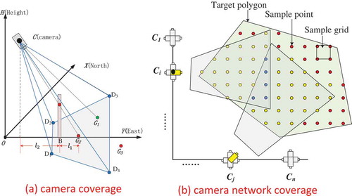
The camera is a directional sensor, whose coverage is mainly decided by parameters such as location, height, the camera’s inner parameters and its gestures. The camera model described in this paper is shown in Figure 1(a), which is expressed as a tuple ; in this tuple, is the position of the camera’s optical centre in the geographic coordinate system; are, respectively, the azimuth angle and the pitch angle. The azimuth angle is the vertical angle between the north direction line of a particular point and the target direction line in the clockwise direction. The pitch angle is the horizontal angle between the vertical direction line of a particular point and the target direction line in the clockwise direction. are respectively the width, height and focal length of the imaging chip. The quadrilateral in grey in Figure 1(a) is the theoretical coverage of the current camera, which is projected from the pyramid formed by C-D₁D₂D₃D₄ to the ground.

Figure 1. Camera coverage model.

A certain spatial point is projected to its corresponding image point , which can be represented by the Formula (1). In the formula, is the scale factor, and does not affect the calculation of image points.

(1)

3.2 Camera coverage model

If a spatial point is covered by a camera, two conditions must be satisfied:

The line of sight intersects the imaging plane. As the coordinates of the spatial point and the camera’s internal and external parameters are known, the coordinates of the image point can be calculated according to Formula (1). When the image coordinates satisfy ,, it indicates that the line of sight intersects the imaging plane. In another word the spatial point must be in the coverage area.

There is no barrier between the spatial point and the imaging plane. As shown in Figure 1(a), a point in the world coordinate system falls within the visible range of the camera, and the line of sight passes through the suspected barrier . is the height of the suspected barrier. The height of the line of sight at can be calculated by H_B, and ,. If , then blocks the line of sight, otherwise does not block the line of sight.

As shown in Figure 1(a) the ground point G₁ is covered, while G₂ and G₃ are not because they do not satisfy one or two above constraints.

3.3 Camera network coverage model

A certain spatial point in the target area can be covered by one or more cameras. As shown in Figure 1(b) the target area is dispersed by grids into sample points. Some of them are not covered by any camera. Some of them are covered by only one camera, while some of them are covered by more cameras. In this paper, if the sample point is covered by any one or more cameras in camera network, then the current spatial point is considered as being covered. And then the coverage of the target area is defined as the ratio of the number of covered points to the total number of sample points shown in formula 2.

(2)

4 Deployment optimization model and method

4.1 Deployment optimization model

4.1.1 Candidate position and posture sampling

As mentioned above a certain camera can be represented by a tuple . In this paper we assume that the internal parameters are known, the five parameters determine that the camera parameter space is a continuous five-dimensional space.

In real geographic environment only limited spaces are suit for camera deployment, which are usually represented as polylines with max and min heights, because the candidate spaces are continuous, and the candidate camera positions are infinite. In this paper the candidate spaces are dispersed which is shown in Figure 2. In Figure 2 the candidate polylines are dispersed into multiple 2D points by a certain step noted as C_step. And then in the vertical direction the height are dispersed by a certain step noted as H_step. Consequently the candidate spaces are sampled into 3D points. The location of a candidate camera are represented as , in which n represents the number of sampled positions.

Figure 2. Candidate position and posture sampling.

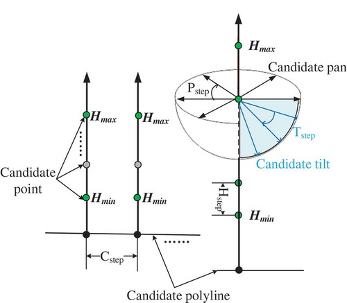
At a certain candidate position only one camera can be deployed with a certain pan and tilt angles in continuous ranges, such as and . In a similar way the pan and tilt angles are dispersed by corresponding steps noted as P_step and T_step, which are shown in Figure 2. Consequently the number of possible pose of a candidate position marked as m can be obtained from Formula (3), where m_P and m_T represent the number of sampled pan and tilt angles, respectively.

(3)

And the pose of a candidate camera can be represented as

4.1.2 Optimization objects

In the paper sampled cameras are noted as , N represents the number of cameras that can be placed and . The target area is sampled into a finite number of points to form a set marked as , in which M is the number of sample points. And then a certain point () in the target area covered by the camera is marked as , and the set of points covered by the camera as .

The goal of optimization for this paper is to use a minimum number of cameras to cover the target area. That is find a subset of the candidate camera set , so that the cameras in can cover sampled points in the target area, while contains the minimum number of cameras. Therefore, the camera deployment optimization model can be expressed as Formula (4), in which represents the number of cameras in the set (the same below), and represents the camera location of the camera :

In Formula (4):

• Target: Select a subset from , with as few elements as possible in .

• Constraint 1: All the sampled points must be covered by at least one camera in .

• Constraint 2: For one position, only one camera can be deployed.

4.2 Deployment optimization method

4.2.1 Model building

According to the optimization model, the optimization process is to select an optimized subset from all the candidate camera sets. This is a permutation problem, and the exhaustive enumeration combination is obviously not feasible. Therefore, the heuristic search method is used to optimize the deployment. In this section, the heuristic search method A* algorithm is used to successively construct the graph structure, cost function and heuristic function of camera deployment optimization.

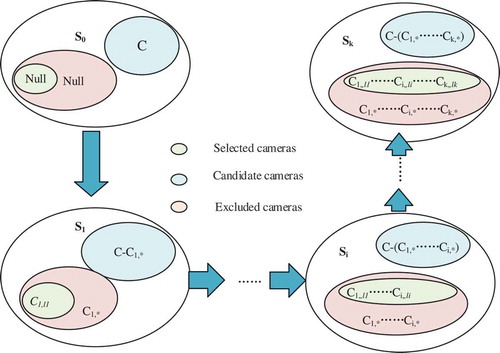
4.2.1.1. Graph structure

Before constructing the graph structure, several tokens should be clarified.

4.2.1.1.1. Selected camera(s)

Selected camera in position i with a certain pose is marked as ,where li represents a certain pan and tilt angle. And the absence of camera in position is marked as . As shown in Figure 3 selected cameras are represented as pentagons filled in green.

Figure 3. Graph structure for cameras.

4.2.1.1.2. Excluded cameras

If camera is selected as one camera in deployment solution, then the other cameras in the same position must be excluded from candidate cameras. In the paper excluded cameras in position i are marked as . As shown in Figure 3 cameras which are located in the same positions with selected cameras are represented as circles filled in red.

4.2.1.1.3. Current candidate cameras

As shown in Figure 3 current candidate cameras are represented as squares filled in blue. The current candidate cameras can be obtained by , where C presents all the candidate cameras and means the cameras in position i.

4.2.1.1.4. State

The combination of all the selected cameras together makes a deployment plan, which is called as a state. The combination after times selections is recorded as . As shown in Figure 3 pentagons filled in green together form a state.

4.2.1.1.5. Coverage of a state

The collection of target spatial points covered by the cameras in the state is marked as . The coverage of the state is marked as , and is expressed as

(5)

4.2.1.1.6. Number of cameras with the maximum coverage

The camera that cover the maximum set of sampled points is marked as , that is,

(6)

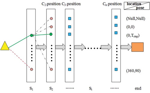
The graph structure is composed of nodes and edges. In the paper all possible states as nodes and the weights of edges between different nodes can be determined by cost and heuristic function mention below. The nodes are the states with selected cameras. The edges between the previous state and current one are determined by cost function. And the edges between current state and next one are determined by heuristic function. Consequently, to construct the graph structure for our method the cost function and heuristic function must can indicate that the process of selection of next state according to current state, which is shown in Figure 4. As shown Figure 4, at the initial state, all cameras are candidate ones and no camera are selected. Then at the state S₁ the camera with max coverage of all cameras are selected. So the next state should involve a new camera in a feasible position with a certain pose which cost less. The process will stop until the satisfied coverage are obtained (Figure 4).

4.2.1.2. Cost function and heuristic function

The cost function and heuristic function must can indicate that the process of selection of next state. As shown in Figure 4, at the initial state, all cameras are candidate ones and no camera is selected. Then at the state S₁ the max coverage of all cameras is selected. So the next state should involve a new camera in a feasible position with a certain pose which cost less. The process will stop until the satisfied coverage is obtained.

Figure 4. The process to find next state.

To ensure that the number is minimum in the next state, the cost function and heuristic function are defined as follows:

4.2.1.2.1. The cost function

The cost of the state is the number of selected cameras, that is, the number of cameras in and is expressed as:

(7)

In which represents a camera is deployed at state i.

4.2.1.2.2. The heuristic function

The expected cost of the state to the optimal object is the number of cameras still needed, which is expressed by the number of spatial points covered by divided by the number of uncovered spatial points:

(8)

4.2.2 Proof

As mentioned above, for A* search algorithm, the conditions of acceptability and consistency should at least be met. This section will prove that the basic structure constructed in this paper meets the requirements.

4.2.2.1. Acceptable conditions proof

Mark the target state as , that is all the sample points have been covered To prove that is not overestimated, it is needed to prove:

(9)

When , , therefore:

Mark , then:

It is proved:

(10)

That is .

4.2.2.2. Consistency condition proof

To prove that current model satisfies the consistency condition, it is needed to prove:

(11)

In which represents the cost from state S_i to S_j. So . And

According to Formula (10), it is known that:

Thereby, it is proved that:

5 Experiment and analysis

5.1 Experiment data and result

In this paper, the experimental area is the northern area of Xianlin campus in Nanjing Normal University, as shown in Figure 5, and the experimental area contains obstacles such as buildings. The experimental data are shapefile format vector data. The red polygons in the Figure 5 are the areas to be monitored (except the basketball court), which includes 15 ones. The orange polylines represent the areas where the candidate cameras can be deployed on, mainly the outer walls of buildings, the edges of roads, etc. These lines all have two attributes named maxH and minH, which are used to represent the maximum and minima height for cameras to be deployed. The grey polygons are the obstacles with an attribute named height, which represents the height of the corresponding building.

Figure 5. Optimal deployment for surveillance cameras.

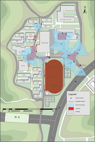
In the experiment, the monitored areas are dispersed into 1 meter × 1 meter grids. Consequently, they are scattered as 6207 spatial points needed to be covered. The areas to deploy cameras are sampled by 1 meter, and the height is sampled every 1 meter. Consequently, they are scattered as 8317 spatial points. Every spatial point is a ‘position’, and on each ‘position’ a number of cameras are set up. They are set up every 20°from 0°to 360°in azimuth angle, and every 10°from 30°to 90°in pitch angle. In words, each ‘position’ has 48 mutually exclusive surveillance cameras. Consequently, 898,236 candidate cameras can be obtained. All the image chips are set to 800 pixels × 600 pixels, and their focal lengths are set to 650 pixels.

Figure 5 shows the deployment plan calculated with the proposed method in the paper. The blue polygons labelled with blue number are the coverage of involved cameras, and the circles filled in blue are the camera positions. The parameters of involved cameras are shown in Table 1.

Table 1. Parameters for candidate cameras.

Camera ID	X (meters)	Y (meters)	H (meters)	P (degree)	T (degree)
1	680,165.625448	3,555,047.626390	2	200	30
2	680,165.661590	3,555,050.626173	3	240	30
3	680,140.897164	3,554,940.792032	8	220	30
4	680,062.676300	3,554,861.521650	7	80	30
5	680,140.723617	3,554,908.792750	6	220	30
6	680,208.030498	3,554,874.238241	5	260	30
7	680,132.412837	3,554,987.559249	10	160	50
8	680,293.102965	3,554,994.687135	18	260	40
9	680,292.954338	3,555,002.557092	10	200	30
10	680,274.954338	3,555,002.557092	14	120	40
11	680,348.826850	3,554,979.193288	2	20	30
12	680,353.362486	3,554,897.144746	8	220	30
13	680,333.458001	3,554,854.859905	6	320	30
14	680,306.783297	3,554,888.023942	8	60	30
15	680,075.410535	3,554,956.976330	2	20	30
16	680,181.382074	3,554,784.170505	6	300	40
17	680,118.574216	3,554,769.473713	4	280	50
18	680,181.603708	3,554,709.768129	2	260	30
19	680,366.825000	3,554,838.722000	5	180	30

5.2. Analysis

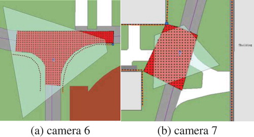
As shown in Figure 5 and Table 1, most of the target areas are covered, and the involved cameras are set in the areas within the feasible heights. There are only 19 cameras are involved, even though there are 898,236 candidate cameras. Consequently, the proposed method can be employed to obtain optimal deployment for camera network with the constraint of geographic environment.

As shown in Figure 6 there are a small number of sample points in the target areas are not covered. That is because the target areas, the candidate positions for camera deployment and the postures of cameras are sampled in certain steps. These uncovered areas can be compensated by manual fine tuning. To sum up, this method can provide technical and decision support for camera deployment optimization.

Figure 6. Details for coverage. (a) Camera 6 and (b) camera 7.

In theory, the smaller grid the target area is separated into, the higher the calculation accuracy of target area coverage is, meanwhile the calculation time will be greatly improved. This paper will disperse the covered target area into 1 meter × 1 meter grid network, which can better fit the target area, but cannot take into account all the target area, with a very small amount of blind spot, which in the future can be resolved by refining the discrete scale.

The position of cameras, the height, the azimuth angle and the sampling accuracy of the pitch angle all affect the final calculation results. In this paper, the coverage of sampled point needs to be calculated 6207 × 898,236 times. It is obvious that it is very time consuming. And then the overlay between different cameras is also time consuming. The time for our experiment is about 4 hours, so our method can be used offline at present. Consequently, the appropriate step should be employed to balance the efficiency and accuracy. If the finer discrete sampling granularity is used, the computational efficiency will be greatly reduced, which will have little impact on offline deployment optimization. If online deployment optimization is needed, one can pre-calculate and store the association between each camera and each sample point with different sampling granularity, speed up the calculation and improve the accuracy of the calculation.

6 Conclusion

n this paper we proposed a method to obtain the optimal deployment of the sensor network in the geographical environment. It takes into consideration the constrain of geographical scene with obstacles, disperses the target areas, the candidate positions, camera parameters according to the actual application requirements, and then makes use of the heuristic search method to cover the target area with as few cameras as possible. The experiment proves the validity and practicability of the method. This method provides technical and decision support for the optimal deployment of cameras and further provides a solution for the deployment of cameras in geographic scenes.

Acknowledgments

The work described in this paper was supported by the National Key Research and Development Program (Grant No. 2016YFE0131600), the National Natural Science Foundation of China (NSFC) (Grant No. 41401442, 41771420).

Disclosure statement

No potential conflict of interest was reported by the authors.

Additional information

Funding

The work described in this paper was supported by the National Key Research and Development Program [Grant No. 2016YFE0131600]; the National Natural Science Foundation of China (NSFC) [Grant No. 41401442, 41771420].

References

- Bouyagoub, S., D. R. Bull, N. Canagarajah, and A. Nix. 2010. “Automatic Multi-Camera Placement and Optimisation Using Ray Tracing.” Proceedings of the 2010 IEEE International Conference on Image Processing, Hong Kong, China, September 26–29.
- Debaque, B., R. Jedidi, and D. Prevost. 2009. “Optimal Video Camera Network Deployment to Support Security Monitoring.” Proceedings of the 12th International Conference on Information Fusion, Seattle, WA, July 6–9.
- Fu, Y.-G., J. Zhou, and L. Deng. 2014. “Surveillance of a 2D Plane Area with 3D Deployed Cameras.” Sensors (Basel, Switzerland) 14 (2): 1988–2011. doi:10.3390/s140201988.
- Hörster, E., and R. Lienhart. 2006. “On the Optimal Placement of Multiple Visual Sensors.” In Proceedings of the 4th ACM International Workshop on Video Surveillance and Sensor Networks, 111–120. Santa Barbara, CA: ACM.
- Ma, H., X. Zhang, and A. Ming. 2009. “A Coverage-Enhancing Method for 3D Directional Sensor Networks.” Proceedings of the IEEE INFOCOM 2009, Rio de Janeiro, Brazil, April 19–25.
- Wang, C., F. Qi, and G.-M. Shi. 2009. “Nodes Placement for Optimizing Coverage of Visual Sensor Networks.” In Advances in Multimedia Information Processing - PCM 2009: 10th Pacific Rim Conference on Multimedia, Bangkok, Thailand, December 15-18, 2009 Proceedings, edited by P. Muneesawang, F. Wu, I. Kumazawa, A. Roeksabutr, M. Liao, and X. Tang, 1144–1149. Berlin, Heidelberg: Springer Berlin Heidelberg.
- Yaagoubi, R., M. E. Yarmani, A. Kamel, and W. Khemiri. 2015. “HybVOR: A Voronoi-Based 3D GIS Approach for Camera Surveillance Network Placement.” ISPRS International Journal of Geo-Information 4: 754–782. doi:10.3390/ijgi4020754.
- Yi-Chun, X., L. Bangjun, and H. EmileA. 2011. “Camera Network Coverage Improving by Particle Swarm Optimization.” EURASIP Journal on Image and Video Processing2011: 458283. doi: 10.1155/2011/458283.
- Yu, T., L. Xiong, M. Cao, Z. Wang, Y. Zhang, and G. Tang. 2016. “A New Algorithm Based on Region Partitioning for Filtering Candidate Viewpoints of A Multiple Viewshed.” International Journal of Geographical Information Science 30 (11): 2171–2187. doi:10.1080/13658816.2016.1163571.
- Zhao, J., H. David, R. Yoshida, and S.-C. S. Cheung. 2011. “Approximate Techniques in Solving Optimal Camera Placement Problems.” Proceedings of the 2011 IEEE International Conference on Computer Vision Workshops (ICCV Workshops), Barcelona, Spain, November 6–13, 1705–1712.
- Zhao, J., and S. Cheung. 2009. “Optimal Visual Sensor Planning.” Proceedings of the 2009 IEEE International Symposium on Circuits and Systems, Taipei, Taiwan, China, May 24–27.