A comparison of three heuristic optimization algorithms for solving the multi-objective land allocation (MOLA) problem

ABSTRACT

Multi-objective land allocation (MOLA) can be regarded as a spatial optimization problem that allocates appropriate use to specific land units concerning some objectives and constraints. Simulating annealing (SA), genetic algorithm (GA), and particle swarm optimization (PSO) have been popularly applied to solve MOLA problems, but their performance has not been well evaluated. This paper applies the three algorithms to a common MOLA problem that aims to maximize land suitability and spatial compactness and minimize land conversion cost subject to the number of units allocated for each use. Their performance has been evaluated based on the solution quality and the computational cost. The results demonstrate that: (1) GA consistently achieves quality solutions that satisfy both the objectives and the constraints and the computational cost is lower. (2) The popular penalty function method does not work well for SA in handling the constraints. (3) The solution quality of PSO needs to be improved. Techniques that better adapt PSO for discrete variables in MOLA problems need to be developed. (4) All three algorithms take high computational costs to achieve quality solutions in handling the objective of maximizing spatial compactness. How to encourage compact allocation is a common problem for them.

KEYWORDS:

• Multi-objective land allocation (MOLA)
• spatial optimization
• genetic algorithm (GA)
• simulated annealing (SA)
• particle swarm optimization (PSO)

1. Introduction

Multi-objective land allocation (MOLA) is a common problem of allocating land units for optimal uses in the planning field. It can be treated as a spatial optimization problem with both spatial and non-spatial objectives (e.g. maximizing land suitability, minimizing land conversion cost, maximizing spatial compactness, minimizing incompatibility between adjacent units) subject to certain constraints (e.g. the total area of the planning space, the target area for each use) (Eastman, Jiang, and Toledano 1998; Coello, Lamont, and Van Veldhuizen 2007; Ligmann-Zielinska, Church, and Jankowski 2008; Liu et al. 2012; Masoomi, Mesgari, and Hamrah 2013).

Due to the multiple non-concordant or conflicting objectives, a large number of possible solutions, and the interdependency between adjacent or proximate land units, exact optimization techniques, such as enumeration, linear programming, branch and bound in integer programming, are not feasible or appropriate to solve MOLA problems (Aerts et al. 2003; Duh and Brown 2007; Ligmann-Zielinska, Church, and Jankowski 2008; Masoomi, Mesgari, and Hamrah 2013; Tong and Murray 2012). Heuristic optimization algorithms have been developed to produce approximate solutions in a reasonable time and have been found applicable to MOLA problems. However, they don’t guarantee the optimal solution (Tong and Murray 2012). Among these heuristic algorithms, simulated annealing (SA), genetic/evolutionary algorithms (GAs/EAs) and particle swarm optimization (PSO) are three popular families (Aerts and Heuvelink 2002; Cao et al. 2011; Cao et al. 2012; Duh and Brown 2005, 2007; Lazoglou, Kolokoussis, and Dimopoulou 2016; Masoomi, Mesgari, and Hamrah 2013; Sahebgharani 2016; Santé-Riveira et al. 2008; Stewart, Janssen, and Van Herwijnen 2004). Because of the nature of the heuristic optimization algorithms, there are some prominent issues and challenges when they are applied to MOLA problems, such as being trapped in local optima, slow rate of convergence and extremely long computation time. Each algorithm has both advantages and pitfalls, and none of them have been proved perfect to solve MOLA problems. An effective and efficient algorithm is expected to consistently achieve quality solutions within a reasonable computation time. It is necessary to compare their performance based on the solution quality and the computational cost so that decision-makers can adopt appropriate algorithm(s) in the future, as well as modify current algorithms to improve their performance.

Except for the classical algorithms in the GA, SA and PSO families, some modified algorithms have also been developed for MOLA problems by incorporating knowledge-informed designations, such as the boundary-based non-dominated sorting genetic algorithm (NSGAII), parallel GA, knowledge-informed Pareto simulated annealing (PSA), multi-objective particle swarm optimization (MOPSO), patch-level PSO, etc. (Cao et al. 2012; Duh and Brown 2007; Liu et al. 2016; Masoomi, Mesgari, and Hamrah 2013; Porta et al. 2013). In this research, we focus on the classical algorithms rather than the modified algorithms based on the following considerations. First, the classical algorithms are flexibly applicable to different MOLA problems, while the modified algorithms are usually designed for specific MOLA problems and sometimes require extra knowledge. For instance, Duh and Brown (2007) designed a knowledge-informed PSA to optimize the allocation of two land uses in a simulated landscape planning problem. The MOPSO and boundary-based NSGAII, developed by Masoomi, Mesgari, and Hamrah (2013) and Cao et al. (2012), respectively, are suitable for optimizing urban land use allocation. The patch-level PSO developed by Liu et al. (2016) needs to incorporate knowledge-rules to guide the land transition. Second, the designation of the modified algorithms is based on the classical algorithms, and their performance also depends on that of the classical algorithms. However, how these classical algorithms perform in solving MOLA problems has not been well evaluated for their solution quality and computational cost. Third, the evaluation of the classical algorithms will help us to answer the following questions: Do these classical algorithms perform well enough in solving MOLA problems? If not, what problems should the modifications focus on? Which classical algorithm is more promising for further improvement?

This paper aims to compare the performance of three popular heuristic optimization algorithms (SA, GA and PSO) in solving the MOLA problem. The three algorithms are applied to a simulated planning area represented with a 30*30 grid, and their performance is evaluated based on the solution quality and the computational cost. The remainder of the paper is organized as follows. Section 2 gives an overview of the three algorithms; Section 3 describes the data and methods used for the test; Section 4 presents and analyses the results; and Section 5 concludes the paper, discusses the limitations and identifies future research directions.

2. An overview of SA, GA and PSO

SA is a single-point search technique for solving combinatorial optimization problems by simulating the thermodynamic process of crystallization (Aerts and Heuvelink 2002; Chen et al. 2007; Duh and Brown 2007; Kirkpatrick, Gelatt, and Vecchi 1983; Nourani and Andresen 1998; Onbaşoğlu and Özdamar 2001; Santé-Riveira et al., 2008). It starts with a randomly generated solution at an initial temperature . Then a neighbour is created by making a small change of the current solution. If the neighbour solution is better, it replaces the current solution. Otherwise, it will be accepted probabilistically. Kirkpatrick, Gelatt, and Vecchi (1983) proposed to follow the Metropolis criterion to decide the acceptance probability given by , where is the acceptance probability, is the difference between the neighbour and the current solution, is the current temperature and is Boltzmann’s constant. The initial temperature should be high enough to accept most transitions, and the probability of accepting deteriorated solutions decreases slowly as the temperature drops. The cooling schedule controls how the acceptance probability decreases. The earliest cooling schedule decreases the temperature by multiplying a cooling factor and has been criticized for the slow rate in finding the near-optimal solution. Other three popular cooling schedules are Boltzmann (logarithmic), Cauchy and quenching (exponential), respectively (Nourani and Andresen 1998; Suman and Kumar 2006). Based on them, the temperature at step is given by , and , respectively. They have been proved faster than the earliest cooling schedule, but suffer the risk of converging to local optima.

GA is a stochastic search technique that simulates the natural selection process. The evolution begins with a population of solutions (individuals). Each solution is associated with a fitness value. The solutions compete to reproduce offspring based on their fitness value and through a set of operators, including selection, crossover and mutation (Coello, Lamont, and Van Veldhuizen 2007). A few parameters influence the performance of GA, including population size, crossover probability and mutation probability. Although appropriate parameter values depend on the problem, researchers agree that a small population size is more likely to result in poor solutions, while a large population size requires longer computation time; the crossover probability was often set between 0.8 and 1.0 and the mutation probability was suggested to be a low value, e.g. 0.01–0.3 (Grefenstette 1986; Haupt 2000; Hesser and Männer 1990). The conventional GA is suitable for solving single-objective optimization problem and has been criticized for the slow rate of convergence. The NSGAII was developed to solve multi-objective optimization problems, as well as to increase the convergence rate and improve the optimization performance (Deb et al. 2000). The fundamental idea of NSGAII is that the solutions are ranked based on non-domination before the selection, crossover and mutation are operated. Compared to the conventional GA, NSGAII has been more popularly applied to MOLA problems and a few modified versions have been developed (Cao et al. 2011, 2012; Lazoglou, Kolokoussis, and Dimopoulou 2016; Porta et al. 2013). Both the conventional GA and the classical NSGAII were tested to solve the MOLA problem, and the performance of NSGAII turned out to be better. Therefore, the classical NSGAII is used as a representation of the GA for the following comparison.

PSO algorithm was designed by simulating the social behaviour of bird flocking or fish schooling. It shares some characteristics of GA, by which a particle and the swarm can be regarded as an individual and a population, respectively. A solution is represented by the position of a particle. For each particle, its position is represented by a D-dimension vector . In one iteration, each particle in the swarm updates its position through updating the flying velocity on each dimension, which makes the particle to move towards its previous best position and the global best position ; can be the best position attained by all particles or the particles in its topological neighbourhood (Banks, Vincent, and Anyakoha 2007; Kitayama and Yasuda 2006; Laskari, Parsopoulos, and Vrahatis 2002; Masoomi, Mesgari, and Hamrah 2013; Sahebgharani 2016). The velocity and position updating in one dimension can be formulated with the following equations:

where and are new and old positions of the particle on dimension , respectively; and are new and old velocities, respectively; and are random numbers in the range [0, 1]; and are cognitive rate and social rate, respectively, which control the relative effect of and , respectively; ; the inertia weight plays the role of balancing global and local search, and is suggested in [0.4, 1.2].

PSO was initially designed for continuous optimization problems. Two approaches have been followed to adapt it for discrete variables. One is to convert the discrete variables into continuous variables. For instance, Masoomi, Mesgari, and Hamrah (2013) use real values in the range (0, 1) to represent the land use content of each cell when applying the MOPSO algorithm to optimize urban land use allocation. The other is to inherently modify the searching and updating strategies (Kitayama and Yasuda 2006; Laskari, Parsopoulos, and Vrahatis 2002; Sahebgharani 2016; Singh, Grandhi, and Stargel 2010). For instance, Laskari, Parsopoulos, and Vrahatis (2002) modified the PSO algorithm by rounding off the real optimum values to their nearest integers after updating a particle’s position, which means that the value of in the position updating equation is rounded to its closest integer. Liu et al. (2016) applied this rounding-off method to the basic PSO algorithm for solving the MOLA problem. Kitayama and Yasuda (2006) proposed a penalty function method that treats discrete variables as continuous variables through penalizing at the intervals. Singh, Grandhi, and Stargel (2010) proposed a technique that controls the values of and in the velocity updating equation to guarantee integer velocity update. Two methods were tested to solve the MOLA problem in this paper, namely converting the discrete variables into continuous variables and rounding off the real optimum values; the latter method performed better. Therefore, the rounding-off method is used for the PSO algorithm in the following comparison.

SA, GA and PSO, as heuristic optimization algorithms, are not guaranteed to achieve optimal solutions in a random run. An effective and efficient algorithm is supposed to consistently achieve quality solutions within a reasonable computation time. The performance of an algorithm should be evaluated by a comprehensive consideration of the solution quality achieved in multiple runs and the computational cost. When these algorithms are run for solving the MOLA problem, an important issue is to determine when the algorithms terminate. More iterations are more likely to make the algorithm to find better solutions, but meanwhile, result in a longer computation time. One arbitrary approach is to manually set the maximum number of iterations. Another approach is to set the algorithm to terminate when it achieves convergence (Greenhalgh and Marshall 2000). Convergence is the state when the solution makes no change with the increasing number of iterations. However, when solving MOLA problems, these algorithms are difficult to achieve absolute convergence because of the large data size and the problem complexity. Researchers have applied a relaxed convergence state for the algorithm termination when solutions make no change within a predefined number of iterations (Duh and Brown 2005; Greenhalgh and Marshall 2000). The number should neither be too high nor too low, since a low value is more likely to make the algorithm trapped in local optima, while a very high value will increase redundant computation with no or little solution improvement.

3. Data and methods

3.1. Data

This study tests the performance of the three algorithms with a semi-hypothetical data set. For the convenience of comparison, a simulated 30*30 grid is used as the planning area with physical and socio-economic characteristics of the land. The planning area is allocated for three land use types, namely agricultural land, construction land and conservation land. The dataset includes three aspects of data, i.e. land suitability data, land conversion cost matrix and current land use data, respectively.

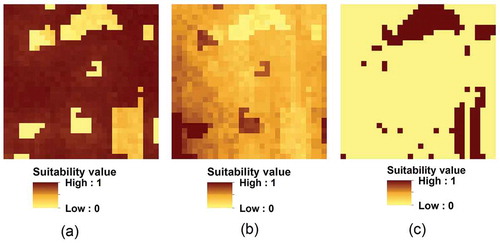
Land suitability data include three raster layers representing to what extent each land unit is suitable for agriculture, construction and conservation, respectively. Land suitability for agriculture and construction was produced by multi-criteria evaluation of physical, socio-economic and ecological factors through the analytic hierarchy process (Satty 2008). The land suitability value of each cell is scalarized to the range [0, 1]; higher value indicates the cell is more suitable for a certain use. Land suitability for conservation is obtained through a (OR) Boolean aggregation of multiple criteria that identify ecologically sensitive or valuable land or other land need to be protected. The land suitability value of each cell is 1 or 0; 1 indicates it is suitable for conservation, while 0 indicates it is not suitable for conservation. This Boolean aggregation method is applied to encourage protection of all ecologically sensitive or valuable areas in the planning area. The multi-criteria selection and evaluation is not the focus of this study. Readers can refer to our previous research for detail information (Song and Chen 2017). The land suitability map for agriculture, construction and conservation is shown in Figure 1(a–c), respectively.

Figure 1. Land suitability maps: (a) Land suitability for agriculture, (b) Land suitability for construction, and (c) Land suitability for conservation.

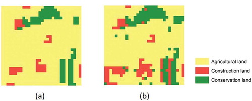
The land conversion cost matrix (Table 1) lists the relative cost of converting a land unit from one (current) use to another (future) use estimated by local experts and planners. Current land use data (Figure 2(b)) is used as a benchmark for calculating the land conversion cost and evaluating the land allocation solutions.

Table 1. Land conversion cost matrix.

	Agriculture	Construction	Conservation
Agriculture	0	0.4	0.8
Construction	1	0	1
Conservation	0.8	0.8	0

Figure 2. Benchmark of solutions: (a) current land use, and (b) solution of the Terrset MOLA procedure under Scenario 1.

3.2. Optimization modelling

MOLA can be represented as a multi-objective combinatorial optimization problem of optimizing (maximizing or minimizing) two or more objectives subject to certain constraints (Coello, Lamont, and Van Veldhuizen 2007). When the target number of units allocated for each land use is an exact value, equal constraints are incorporated into the optimization model; otherwise, the model incorporates non-equal constraints. Two approaches have been developed to solve multi-objective optimization problems. One is the weighted combination of multiple objectives, which converts the multi-objective problem to a single-objective one, and achieves a single solution under a given weighting scheme. The other approach deals with the multiple objectives simultaneously by searching non-dominated solutions, by which none of the objectives can be improved without degrading some other objectives. This study solves the problem by following the multi-objective weighted combination approach. Three objectives are considered: maximizing land suitability, maximizing spatial compactness, and minimizing land conversion cost, respectively. The target number of units allocated for agricultural land, construction land, and conservation land are regarded as constraints.

3.2.1. The optimization model

1. Objective 1: Maximizing land suitability.

Maximize :

(1)

1. Objective 2: Maximizing spatial compactness. It is represented by maximizing the number of cells allocated for the same use in each cell’s eight neighboring cells (Aerts et al. 2003; Cao et al. 2012; Ligmann-Zielinska, Church, and Jankowski 2008).

Maximize :

(2)

where

(3)

1. Objective 3: Minimizing land conversion cost.

Minimize :

(4)

1. A weighted combination of Objective 1, Objective 2 and Objective 3:

Maximize :

(5)

1. Constraints:

(6)

In the above formulas, is the number of land use types, and . and are the total number of rows and columns of the planning area, respectively, and = = 30. when the cell is allocated for land use , =1; otherwise, is the weight given to land use ; . is the suitability level of cell used for land use . is the land conversion cost when cell is allocated for land use . is the integrated objective function value (OFV). , and are the OFVs of objectives 1–3, respectively. , and are the weights given to objectives 1–3, respectively. is the target number of cells allocated for land use . The numbers of cells used for agricultural land, construction land and conservation in current land use are 738, 56 and 108, respectively. Considering the tendency of construction sprawl and the objective of protecting current conservation land, we set the target number of units allocated for the three land use types as 650, 110 and 140, respectively.

3.2.2. Constraint handling method

The constraints of the optimization model are the target numbers of cells allocated for agricultural land, construction land, and conservation land respectively. When a solution satisfies all the constraints, it is regarded as a feasible solution; otherwise, it is regarded as infeasible. The most popular constraint handling method is the use of penalty functions, by which the objective function is augmented with penalties proportional to the degree of constraint violations (CVs) (Coello, Lamont, and Van Veldhuizen 2007). This method is applied in our test.

Maximize OFV:

(7)

where

(8)

In formulas (7) and (8), is the augmented OFV, is the penalty factor and is the constraint violation. The value of keeps constant in the three algorithms under the same scenario, but varies with scenarios depending on the relative values of and . of a feasible solution is zero; higher values indicate poorer solution quality.

3.3. Scenario design, programming and tools

Three scenarios are designed to represent different weighting schemes in formula (5). Under the three scenarios, the value of the penalty factor in formula (7) also differs.

Scenario 1: . Scenario 1 only deals with the non-spatial objective of maximizing land suitability. The objective function is linear.

Scenario 2: . Scenario 2 only deals with the spatial objective of maximizing spatial compactness. The objective function is non-linear.

Scenario 3: p = 0.5. Scenario 3 deals with the combination of the objectives of maximizing land suitability, maximizing spatial compactness and minimizing land conversion cost. The objective function is non-linear. The weighting scheme is applied because the land allocation patterns generated by the three algorithms are more satisfactory based on our visual interpretation when planning rationality and spatial compactness are considered.

When stochastic algorithms are applied to solve optimization problems, appropriate initial solutions will increase the convergence rate and guide the algorithms to find quality solutions (Cao et al. 2011; Duh and Brown 2007; Masoomi, Mesgari, and Hamrah 2013). Consider the MOLA context, instead of using totally random initial solutions, we created initial solutions by randomly altering 50% of current land use. We compared this method with the random initialization method. It turned out to decrease the computation time without degrading the solution quality.

Inspyred, a python open-source library, is used for running the algorithms. ARCGIS 10.3 is used for mapping and displaying the solutions. The algorithms are computed on a computer with Intel Core i7-3770 [email protected].

3.4. Methods for evaluating algorithm performance

The algorithms are set to terminate when the relaxed convergence state is achieved. Among the three algorithms, SA searches a single-solution in one iteration, while PSO and GA search multiple solutions. Considering this, we set the three algorithms to terminate when the best solution achieved makes no change after 10,000 solutions have been searched. The value is set to make a compromise of the solution quality and the computational cost. The performance of the algorithms under each scenario is evaluated based on the solution quality and the average computational cost in 20 runs.

The computational cost is evaluated based on the number of solutions that have been searched (evaluated) and the associated computation time. More searched solutions and longer computation time indicate higher computational cost.

The solution quality is evaluated based on the augmented OFV, the CV and the mapping of the solution. The OFV of a quality solution should be high and close to that of the estimated optimal solution. The CV of a quality solution should be zero or near zero, which indicates it satisfies or slightly violates the constraints. For Scenario 2, the mappings of the solutions are visually compared to the estimated optimal land allocation pattern, in which all cells allocated for the same use cluster into a single patch, and the shape of the patch is close to rectangular. For Scenarios 1 and 3, they are compared to the current land use pattern (Figure 2(a)) to determine whether they fulfil the following planning rationality criteria: (a) current conservation land is preserved in the land allocation result, (b) current construction land keeps its type and (c) new construction land tends to be allocated next to current construction land. The three criteria are defined based on the following planning considerations. First, current conservation land is supposed to be protected from construction and agricultural activities. Second, the conversion from construction land to conservation or agricultural land is possible, but seldom happens, and the conversion cost is usually very high. Third, future construction is expected to be allocated adjacent to current construction land to take advantage of the existing infrastructure. In a quality solution, most cells should fulfil the three criteria. In addition, the MOLA procedure in the TerrSet software adopts a heuristic searching procedure to maximize land suitability. Its solution (Figure 2(b)) is also used as a benchmark for evaluating the solutions under Scenario 1.

4. Results

SA, GA and PSO were run for solving the MOLA problem under the three scenarios, respectively. Each algorithm has run for 20 times. The statistics of the OFVs, the CVs, the number of searched solutions and the computation time were summarized in Table 2. The OFVs of all solutions under each scenario were plotted in Figure 3. Under each scenario, the solutions with the highest and lowest OFVs achieved by each algorithm were identified and mapped in Figures 4–6 respectively.

Table 2. The statistics of OFVs, CVs, the number of searched solutions and computation time under each scenario.

	Scenario 1			Scenario 2			Scenario 3
	SA	GA	PSO	SA	GA	PSO	SA	GA	PSO
Maximum OFV	751.19	752.03	751.63	823.6	829.1	827.13	494.58	494.76	488.77
Minimum OFV	747.26	750.88	744.17	714.23	786.73	772.88	486.45	487.8	480.92
Average OFV	750.27	751.58	748.45	765.88	807.98	802.62	492.73	491.34	484.87
SD of OFVs	0.83	0.42	2.02	28.62	9.71	13.37	1.8	2.06	2.51
Number of solutions with zero CV	20	20	20	0	20	20	16	20	20
Average number of searched solutions	168,384	219,900	453,595	344,882	226,515	348,615	248,730	201,830	252,465
Average computation time (s)	482.2516	1061.297	1732.33	4140.056	3129.277	4411.579	2992.226	2813.994	3311.852

Figure 3. OFVs of solutions from multiple runs under each scenario: (a) OFVs under Scenario 1, (b) OFVs under Scenario 2 and (c) OFVs under Scenario 3.

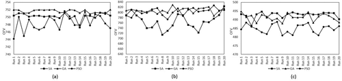
Figure 4. Solutions with highest OFV and lowest OFV under Scenario 1: (a) solution of SA with highest OFV, (b) solution of SA with lowest OFV, (c) solution of GA with highest OFV, (d) solution of GA with lowest OFV, (e) solution of PSO with highest OFV and (f) solution of PSO with lowest OFV.

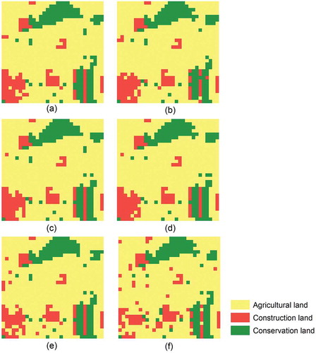
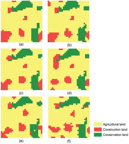
Figure 5. Solutions with highest OFV and lowest OFV under Scenario 2: (a) solution of SA with highest OFV, (b) solution of SA with lowest OFV, (c) solution of GA with highest OFV, (d) solution of GA with lowest OFV, (e) solution of PSO with highest OFV and (f) solution of PSO with lowest OFV.

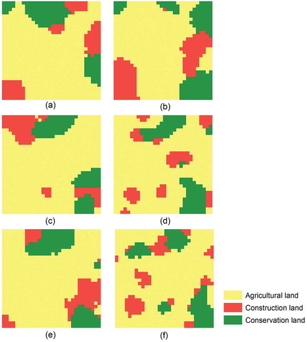
Figure 6. Solutions with highest OFV and lowest OFV under Scenario 3: (a) solution of SA with highest OFV, (b) solution of SA with lowest OFV, (c) solution of GA with highest OFV, (d) solution of GA with lowest OFV, (e) solution of PSO with highest OFV and (f) solution of PSO with lowest OFV.

4.1. Solution quality

4.1.1. OFVs and CVs of solutions

Under Scenario 1, the objective is to maximize land suitability subject to the target number of units allocated for each use. The solution that maximizes the objective function regardless of the constraints has an OFV of 771.04. The solution generated by the TerrSet MOLA procedure has an OFV of 749.55 (Figure 2(b)). We can safely estimate the optimal solution that maximizes the objective function while satisfying the constraints has an OFV in the range [749.55, 771.04). Among 20 runs, all the three algorithms converge to feasible solutions with zero CVs. The maximum OFVs of the three algorithms are all higher than 749.55, while only the minimum OFV of GA is higher than 749.55. The average OFVs of GA and SA are both higher than 749.55, while that of PSO is lower than 749.55. The variation of OFVs in multiple runs of PSO is obviously larger than that of GA and SA.

Under Scenario 2, the objective is to maximize spatial compactness subject to the target number of units allocated for each use. Among 20 runs, GA and PSO always converge to feasible solutions with zero CVs, while SA converges to solutions with non-zero CVs. This indicates that the penalty function method doesn’t work well for SA in handling the constraints; it is very likely to converge to infeasible solutions. The average OFVs of the three algorithms are ranked as GA>PSO>SA, while the variations of solutions among multiple runs are ranked as SA>PSO>GA. The maximum OFVs of the three algorithms are close, while the minimum OFV of SA is obviously lower because of the penalty applied to infeasible solutions.

Under Scenario 3, the three objectives of maximizing land suitability, maximizing spatial compactness and minimizing land conversion cost are weighted combined. Among 20 runs, GA and PSO always converge to feasible solutions with zero CVs. SA converges to four solutions with non-zero CVs, but the CV values are 2 or 4, very close to zero, which indicates that the solutions slightly violate the constraints. For GA and SA, their maximum, minimum and average OFVs are very close, while the OFVs of PSO are obviously lower. The variations of solutions among multiple runs are ranked as SA<GA<PSO.

4.1.2. Mapping of solutions

Under Scenario 1, the mappings of the solutions (Figure 4) are compared to current land use (Figure 2(a)). In the six solutions, most cells fulfill the three planning rationality criteria. The main problem is that some isolated cells are allocated for new construction land, but they are not adjacent to current construction land. For each algorithm, the number of isolated cells in the solution with the lowest OFV is more than that in the solution with the highest OFV. When the solutions of the three algorithms are compared, the number of isolated cells in the solution of PSO is obviously more. This indicates that the solution quality of PSO is not as good as that of SA and GA. The isolated cells also indicate that the optimization model that only considers the objective of maximizing land suitability cannot generate desirable planning maps.

Under Scenario 2, the mappings of the solutions (Figure 5) are visually interpreted to determine their closeness to the estimated optimal pattern, in which all cells allocated for the same use cluster into a single patch and the shape of the patch is close to rectangular. All six solutions fail to achieve the optimal land allocation pattern. In all six solutions, the cells allocated for the same use tend to cluster, while the number and the shape of the clusters (patches) differ. For each algorithm, the solution with the highest OFV has less patches than that with the lowest OFV. When the three algorithms are compared, the three solutions with the highest OFVs (Figure 5(a,c,e)) have the similar number of patches; the numbers of patches in the solutions with the lowest OFVs (Figure 5(b,d,f)) greatly differ, and are ranked as SA<GA<PSO. The solutions of SA are visually more compact.

Under Scenario 3, the land allocation patterns in the three solutions with the highest OFVs (Figure 6(a,c,e)) are globally similar but show local differences. The solution of GA fulfils the three planning rationality criteria. In the solution of SA, there are two cells violating the three criteria: one cell of conservation land has been converted to construction land, and one cell of construction land has been converted to conservation land. In the solution of PSO, one isolated cell is used for agricultural land inside the construction patch; one isolated cell and one isolated patch allocated for new construction are not adjacent to current construction land. This indicates all the three algorithms are possible to converge to quality solutions that fulfil or slightly violate the planning rationality criteria under this scenario. However, the solutions with the lowest OFVs (Figure 6(b,d,f)) are visually very different. Compared to the solutions with the highest OFVs, the allocation of construction land in these three solutions is more scattered, resulting in more patches. Some of these patches are adjacent to current construction land, but some are not. The solution of GA fulfils the planning rationality criteria, and the shape of the patches is more close to rectangular. There is one isolated patch allocated for new construction land in the solution of SA. In the solution of PSO, the number of these isolated patches or cells is more, and the shape of the patches is less compact.

4.2. Computational cost

According to Table 2, under Scenario 1, the average numbers of searched solutions of GA and SA are close, but the computation time of GA doubles that of SA. The GA (NSGAII) applied in our test ranks all the solutions based on non-domination before the selection, crossover and mutation are operated. This improves the optimization performance, but increases the computation time. The average number of searched solutions of PSO is obviously larger than that of GA and SA, which results in a longer computation time. To summarize, under Scenario 1, the computational cost of SA is the lowest, while that of PSO is the highest.

Under Scenario 2, the average computation time of the all three algorithms is obviously longer than those under Scenario 1. Since the objective function is non-linear under Scenario 2, it takes longer time for each algorithm to evaluate a single solution. Among the three algorithms, the average number of searched solution of GA is obviously less than that of PSO and SA. As a result, its computation time is the shortest.

Under Scenario 3, the average number of searched solutions of GA is obviously less than that of PSO and GA. As a result, its computation time is the shortest among the three, but it still costs 46 min. The computation time of PSO is the longest, since it needs to search more solutions to achieve convergence.

5. Conclusions and discussions

This paper compares the performance of three heuristic algorithms in solving a common MOLA problem, including simulated annealing (SA), GA and PSO, respectively. The MOLA aims to maximize land suitability and spatial compactness, and minimize land conversion cost subject to the target number of units allocated for each use. Three scenarios are designed: Scenarios 1 and 2 independently consider the two objectives of maximizing land suitability and maximizing spatial compactness, respectively, while Scenario 3 considers the three objectives simultaneously. The performance of the three algorithms were tested with a simulated planning area represented by a 30*30 grid, and evaluated based on the solution quality and the computational cost.

Under Scenarios 1 and 3, GA consistently converges to quality solutions that satisfy both the objectives and the constraints, and meanwhile fulfils the planning rationality; most solutions generated by SA also satisfy the objectives and the planning rationality, but a few solutions violate the constraints; the solutions of PSO need improvement. Under Scenario 2, none of the three algorithms guarantees the estimated optimal solution in which the cells allocated for the same land use are completely contiguous, but all of them can maintain a certain level of spatial compactness.

Under Scenarios 2 and 3 which consider the objective of maximizing spatial compactness, all the three algorithms takes a high computational cost to converge to quality solutions. Among the three algorithms, GA achieves a quicker convergence, but it still takes 53 and 46 min under Scenarios 2 and 3, respectively.

When the solution quality and the computational cost under all scenarios are comprehensively considered, GA performs best among the three algorithms. However, all the three algorithms have difficulties in handling the spatial objective of maximizing spatial compactness. GA and SA can converge to quality solutions but the computational cost is high, while the compactness level of the solutions generated by PSO needs improvement. This indicates that to improve their capability in maintaining spatial compactness is a common problem for all three algorithms to improve their performance in solving MOLA problems. Some research has been done to encourage compact land allocation by incorporating knowledge-informed rules to the classical GA, SA and PSO algorithms. Some researchers designed one or two operators based on simple rules: For instance, Duh and Brown (2007) incorporated the compactness and contiguity rules into the SA algorithm to encourage compact land allocation by determining the land use type of a cell based on its neighbouring cells. Some researchers designed a series of knowledge-informed operators for the classical algorithms: Cao et al. (2012) designed a series of boundary-based operators for NSGAII to guide compact land allocation to encourage land use change to happen on the boundary cells of patches, instead of the core cells; Datta et al. (2007) developed a series of knowledge-informed operators for NSGAII by incorporating the patch-based, edge growing/decreasing and neighbourhood rules to encourage compact land allocation. However, it is unclear that which approach performs better. Whether should it incorporate simple operators or a series of complex operators? Will incorporating a series of operators really improve the computation efficiency considering the computation cost of the operators themselves? Future research needs to answer these questions.

The penalty function method is applied in our test to handle the constraints in the optimization problem, because it can work on all three algorithms without changing their searching mechanisms. Based on the test, it works well for PSO and GA, but not well for SA, especially under Scenario 2. In previous studies that applied SA algorithms to solve MOLA problems, the target numbers of units allocated for each land use are usually exact values or percentages. The number of units allocated for each use were set in the initial solutions and kept unchanged during the solution update (Aerts and Heuvelink 2002; Duh and Brown 2005, 2007; Santé et al. 2016). No penalty function is needed for this approach and the constraint violation problem can be avoided. However, the poor flexibility will prevent this method from solving MOLA problems when the target number of units allocated for each use is a range of values constrained by the upper and lower limits, while this is often the case in many real-life planning problems. Therefore, to improve the performance and flexibility of SA in solving MOLA problems, effective constraint handling techniques need to be developed. One possible method is to incorporate knowledge-informed rules to the mutation operators to steer infeasible solutions towards feasible ones during the solution searching.

For PSO, even under Scenario 1 when the spatial pattern of land allocation is not considered, the quality of its solutions needs improvement. PSO has been proven effective in solving continuous optimization problems, while MOLA is a combinatorial optimization problem. We adopted a rounding-off method to adapt it for discrete variables. This rounding-off method has been applied in previous research and has performed better than the method of converting discrete variables to continuous ones (Laskari, Parsopoulos, and Vrahatis 2002; Liu et al. 2016; Masoomi, Mesgari, and Hamrah 2013). However, the rounding-off method still doesn’t perform well enough to obtain quality solutions. Therefore, to improve the performance of PSO in solving MOLA problems, except for the modifications to encourage compact land allocation, effective techniques that adopt the algorithm for discrete variables need to be developed and applied. For instance, Kitayama and Yasuda (2006) proposed a penalty function method that treats discrete variables as continuous variables through penalizing at the intervals. Singh, Grandhi, and Stargel (2010) proposed a technique that controls the random values in the velocity updating equation to guarantee integer velocity update. Whether these methods will improve the performance of PSO in solving MOLA problems requires further research.

In this study, we focus on the classical algorithms in the SA, GA and PSO families. However, there are other heuristic optimization algorithms applicable to MOLA problems. For instance, ant colony optimization (ACO) has also been proven effective in solving some spatial optimization problems, such as the traveling salesman problem, network routing problem, facility siting problem, etc. (Li, He, and Liu 2009). However, the classical ACO only implements one type of ants. It is suitable to find optimal sites for a single land use, while not effective to optimize multiple land allocations. Liu etal. (2012) have developed a multi-type ant colony optimization (MACO) algorithm for MOLA. It has been proven more efficient than classical GA and SA, while its performance has not been compared to that of the modified SA, GA and PSO algorithms. One limitation of the algorithm is that it can only provide a single solution under a given trade-off scheme between the multiple objectives. Future study will be needed to further compare the modified versions of SA, GA and PSO and other algorithms such as MACO to evaluate their effectiveness and efficiency.

Considering the computation cost, this study applies the three algorithms to a simulated planning area of 30*30 grid for the convenience of comparison. If the test is done with a real-life planning area, the larger dataset will make it difficult for the algorithms to achieve convergence. We have to manually decide when the iteration should terminate to make a compromise between the solution quality and the computational cost. In addition, the optimal solution in a real-life planning problem is usually unknown, and it will be more challenging to evaluate the solution quality. More uncertain factors would, therefore, be introduced and make the comparison more complex. Moreover, an algorithm that accidentally achieves quality solutions will not be regarded as effective and efficient in solving the problem. Therefore, we have compared the performance of the algorithms based on their solution quality and computational cost in multiple runs with a simulated dataset. The main contributions of this research is to help us get a better understanding on the advantages and limitations of these popularly applied algorithms and the directions for further improving the algorithms. More research will be needed to improve and apply these algorithms to solve real-life planning problems.

Disclosure statement

No potential conflict of interest was reported by the authors.

References

- Aerts, J. C. J. H., E. Eisinger, G. B. M. Heuvelink, and T. Stewart. J. 2003. “Using Linear Integer Programming for Multi-Site Land-Use Allocation.” Geographical Analysis 35 (2): 148–169. 10.1111/j.1538-4632.2003.tb01106.x.
- Aerts, J. C. J. H., and G. B. M. Heuvelink. 2002. “Using Simulated Annealing for Resource Allocation.” International Journal of Geographical Information Science 16 (6): 571–587. 10.1080/13658810210138751.
- Banks, A., J. Vincent, and C. Anyakoha. 2007. “A Review of Particle Swarm Optimization. Part I: Background and Development.” Natural Computing 6 (4): 467–484. doi:10.1007/s11047-007-9049-5.
- Cao, K., M. Batty, B. Huang, Y. Liu, L. Yu, and J. Chen. 2011. “Spatial Multi-Objective Land Use Optimization: Extensions to the Non-Dominated Sorting Genetic algorithm-II.” International Journal of Geographical Information Science 25 (12): 1949–1969. doi:10.1080/13658816.2011.570269.
- Cao, K., B. Huang, S. Wang, and H. Lin. 2012. “Sustainable Land Use Optimization Using Boundary-Based Fast Genetic Algorithm.” Computers, Environment and Urban Systems 36 (3): 257–269. doi:10.1016/j.compenvurbsys.2011.08.001.
- Chen, D., C. Lee, C.-H. Park, and P. Mendes. 2007. “Parallelizing Simulated Annealing Algorithms Based on High-Performance Computer.” Journal of Global Optimization 39 (2): 261–289. doi:10.1007/s10898-007-9138-0.
- Coello, C. A. C., G. B. Lamont, and D. A. Van Veldhuizen. 2007. Evolutionary Algorithms for Solving Multi-Objective Problems. Vol. 5. New York: Springer.
- Datta, D., K. Deb, C. M. Fonseca, F. G. Lobo, P. A. Condado, and J. Seixas. 2007. “Multi-Objective Evolutionary Algorithm for Land-Use Management Problem.” International Journal of Computational Intelligence Research 3 (4): 371–384. 10.5019/j.ijcir.2007.118.
- Deb, K., S. Agrawal, A. Pratap, and T. Meyarivan. 2000. “A Fast Elitist Non-Dominated Sorting Genetic Algorithm for Multi-Objective Optimization: NSGA-II.” Lecture Notes in Computer Science 1917: 849–858.
- Duh, J. D., and D. G. Brown. 2005. “Generating Prescribed Patterns in Landscape Models.” In GIS, Spatial Analysis and Modeling, Eds. D. J. Maguire and M. F. Goodchild, 423–444, ESRI Press.
- Duh, J. D., and D. G. Brown. 2007. “Knowledge-Informed Pareto Simulated Annealing for Multi-Objective Spatial Allocation.” Computers, Environment and Urban Systems 31 (3): 253–281. 10.1016/j.compenvurbsys.2006.08.002.
- Eastman, J. R., H. Jiang, and J. Toledano. 1998. Multi-criteria and multi-objective decision making for land allocation using GIS. In Multicriteria Analysis for Land-Use Management. Environment & Management, vol 9, edited by E. Beinat and P. Nijkamp. Dordrecht: Springer. doi:10.1007/978-94-015-9058-7_13.
- Greenhalgh, D., and S. Marshall. 2000. “Convergence Criteria for Genetic Algorithms.” SIAM Journal on Computing 30 (1): 269–282. doi:10.1137/S009753979732565X.
- Grefenstette, J. J. 1986. “Optimization of Control Parameters for Genetic Algorithms.” IEEE Transactions on Systems, Man, and Cybernetics 16 (1): 122–128. doi:10.1109/TSMC.1986.289288.
- Haupt, R. L. (2000). Optimum Population Size and Mutation Rate for a Simple Real Genetic Algorithm That Optimizes Array Factors. In Antennas and Propagation Society International Symposium, 2000. IEEE (Vol. 2, pp. 1034–1037).
- Hesser, J., and R. Männer (1990). Towards an Optimal Mutation Probability for Genetic Algorithms. In International Conference on Parallel Problem Solving from Nature (pp. 23–32).
- Kirkpatrick, S., C. D. Gelatt, and M. P. Vecchi. 1983. “Optimization by Simulated Annealing.” Science 220 (4598): 671–680. doi:10.1126/science.220.4598.671.
- Kitayama, S., and K. Yasuda. 2006. “A Method for Mixed Integer Programming Problems by Particle Swarm Optimization.” Electrical Engineering in Japan 157 (2): 40–49. doi:10.1002/(ISSN)1520-6416.
- Laskari, E. C., K. E. Parsopoulos, and M. N. Vrahatis (2002). Particle Swarm Optimization for Integer Programming. Proceedings of the 2002 Congress on Evolutionary Computation. CEC’02 (Cat. No.02TH8600), 2, 1582–1587. 10.1109/CEC.2002.1004478
- Lazoglou, M., P. Kolokoussis, and E. Dimopoulou. 2016. “Investigating the Use of a Modified NSGA-II Solution for Land-Use Planning in Mediterranean Islands.” Journal of Geographic Information System 8 (3): 369–386. doi:10.4236/jgis.2016.83032.
- Li, X., J. He, and X. Liu. 2009. “Intelligent GIS for Solving High-Dimensional Site Selection Problems Using Ant Colony Optimization Techniques.” International Journal of Geographical Information Science 23 (4): 399–416. doi:10.1080/13658810801918491.
- Ligmann-Zielinska, A., R. L. Church, and P. Jankowski. 2008. “Spatial Optimization as a Generative Technique for Sustainable Multiobjective Land-Use Allocation.” International Journal of Geographical Information Science 22 (6): 601–622. doi:10.1080/13658810701587495.
- Liu, X., X. Li, X. Shi, K. Huang, and Y. Liu. 2012. “A Multi-Type Ant Colony Optimization (MACO) Method for Optimal Land Use Allocation in Large Areas.” International Journal of Geographical Information Science 26 (7): 1325–1343. doi:10.1080/13658816.2011.635594.
- Liu, Y., J. Peng, L. Jiao, and Y. Liu. 2016. “PSOLA: A Heuristic Land-Use Allocation Model Using Patch-Level Operations and Knowledge-Informed Rules.” PLoS ONE 11 (6): 1–21. 10.1371/journal.pone.0157728.
- Masoomi, Z., M. S. Mesgari, and M. Hamrah. 2013. “Allocation of Urban Land Uses by Multi-Objective Particle Swarm Optimization Algorithm.” International Journal of Geographical Information Science 27 (3): 542–566. doi:10.1080/13658816.2012.698016.
- Nourani, Y., and B. Andresen. 1998. “A Comparison of Simulated Annealing Cooling Strategies.” Journal of Physics A: Mathematical and General 31 (41): 8373–8385. doi:10.1088/0305-4470/31/41/011.
- Onbaşoğlu, E., and L. Özdamar. 2001. “Parallel Simulated Annealing Algorithms in Global Optimization.” Journal of Global Optimization 19 (1): 27–50. doi:10.1023/A:1008350810199.
- Porta, J., J. Parapar, R. Doallo, F. F. Rivera, I. Santé, and R. Crecente. 2013. “High Performance Genetic Algorithm for Land Use Planning.” Computers, Environment and Urban Systems 37: 45–58. doi:10.1016/j.compenvurbsys.2012.05.003.
- Sahebgharani, A. 2016. “Multi-Objective Land Use Optimization through Parallel Particle Swarm Algorithm: Case Study Baboldasht District of Isfahan, Iran.” Journal of Urban and Environmental Engineering 10 (1): 42–49. doi:10.4090/juee.
- Santé, I., F. F. Rivera, R. Crecente, M. Boullón, M. Suárez, J. Porta, and R. Doallo. 2016. “A Simulated Annealing Algorithm for Zoning in Planning Using Parallel Computing.” Computers, Environment and Urban Systems 59: 95–106. 10.1016/j.compenvurbsys.2016.05.005.
- Santé-Riveira, I., M. Boullón-Magán, R. Crecente-Maseda, and D. Miranda-Barrós. 2008. “Algorithm Based on Simulated Annealing for Land-Use Allocation.” Computers & Geosciences 34 (3): 259–268. 10.1016/j.cageo.2007.03.014.
- Satty, T. L. 2008. “Relative Measurement and Its Generalization in Decision Making: Why Pair Wise Comparisons Are Central in Mathematics for the Measurement of Intangible factors-The Analytic Hierarchy Process.” Racsam 102 (2): 251–318. doi:10.1007/BF03191825.
- Singh, G., R. V. Grandhi, and D. S. Stargel. 2010. “Modified Particle Swarm Optimization for a Multimodal Mixed-Variable Laser Peening Process.” Structural and Multidisciplinary Optimization 42 (5): 769–782. doi:10.1007/s00158-010-0540-8.
- Song, M., and D. Chen. (2017). Establishing a Comprehensive Land Suitability Evaluation System for “Multi-Plan Integration” in China’s County-Level Division. Manuscript submitted for publication.
- Stewart, T. J., R. Janssen, and M. Van Herwijnen. 2004. “A Genetic Algorithm Approach to Multiobjective Land Use Planning.” Computers & Operations Research 31 (14): 2293–2313. 10.1016/S0305-0548(03)00188-6.
- Suman, B., and P. Kumar. 2006. “A Survey of Simulated Annealing as A Tool for Single and Multiobjective Optimization on JSTOR.” Journal of the Operational Research Society 1143–1160. 10.1057/palgrave.jors.2602068.
- Tong, D., and A. T. Murray. 2012. “Spatial Optimization in Geography.” Annals of the Association of American Geographers 102 (6): 1290–1309. doi:10.1080/00045608.2012.685044.