Predicting land use/cover change in Long Island Sound Watersheds and its effect on invasive species: a case study for glossy buckthorn

ABSTRACT

Land use/cover change (LUCC) is a major threat to ecosystems. It may affect the abundance and distribution of species. Despite the importance of LUCC to ecological patterns and processes, few quantitative projections are available for use in ecological modelling. To fill in this literature gap, we constructed a LUCC model for Long Island Sound Watersheds (LISW) and explored the potential effect of the future LUCC on the range size of an invasive species (glossy buckthorn, Frangula alnus). We first applied the multi-layer perceptron–Markov chain model to predict the future LUCC in the LISW area within New England, USA, and then used the predicted land use/cover data as input into a species distribution model to simulate the future range size of glossy buckthorn. Our results indicate that under the current LUCC trend, there is a continued loss of forest and an increase of developed land in the near future, and this LUCC affects the relative suitability for glossy buckthorn.

KEYWORDS:

• Land use/cover change
• invasive species
• glossy buckthorn
• Long Island Sound Watersheds

1. Introduction

Land use/cover change (LUCC) is a major threat to ecological systems and biological diversity. LUCC can cause changes in the provision and values of some ecosystem services (Polasky et al. 2011). For example, carbon sequestration is one of ecosystem services that is dependent on land-use change (Schulp, Nabuurs, and Verburg 2008; Hobbs et al. 2016). Carbon sequestration has a significant impact on climate and nutrient retention regulation (Polasky et al. 2011). Padilla et al. (2010) studied the implications of land-use change on carbon sequestration services and found that woodland conservation is vital to maintaining ecosystem functions that underlie carbon sequestration. For another example, pollination service is another ecosystem service affected by LUCC. LUCC may have direct and indirect effects on pollinator community composition and pollination service. It may also impact wild pollinator abundance and diversity. Habitat loss caused by LUCC may be susceptible to pollination failure (Ricketts et al. 2008; Cusser, Neff, and Jha 2016). Therefore, potential ecological consequences should be considered in land management practices and land use decision-making processes.

On the other hand, changes in LUCC may cause fragmentation, degradation, isolation and even loss of habitats, which may further cause the declines of biodiversity. Sala et al. (2000) simulated the scenarios of global biodiversity changes for the year 2100 and predicted that among the major impact factors (e.g. climate change, nitrogen deposition, biotic exchange and elevated carbon dioxide concentration), land use change probably would have the largest effect on the changes of biodiversity of terrestrial ecosystems. Jetz, Wilcove and Dobson (2007) projected the impact of climate and LUCC on the global diversity of birds and declared that climate change might seriously affect biodiversity; but in the near future, LUCC in tropical countries probably would cause greater species loss. De Chazal and Rounsevell (2009) suggested that studying interactions and feedbacks between biodiversity and LUCC should be conducted.

LUCC may affect the abundance and distribution of species. Many researches have been conducted to study how species respond to LUCC. For example, Paul and Meyer (2001) summarized previous studies about the effects of landscape transformations on stream ecosystems and concluded that increase in urbanized surfaces leads to consistent decline of the richness of algal, invertebrate and fish communities in urban streams. For another example, Marzluff (2008) studied the relationship between bird diversity and decrease of forest cover in Seattle. One of his findings is that extinction of native forest birds increases linearly with loss of forest. More recently, Cousins et al. (2015) examined the effects of LUCC from 1900 to 2013 in a region within south-eastern Sweden and found that the increased species richness was related to the presence of grassland habitats and increased landscape heterogeneity.

As aforementioned, LUCC is a major threat to ecological systems and biological diversity, and by far, human-induced modifications are the most significant modern forces to LUCC. Therefore, predicting future landscape change and forecasting its effect on species are important for conserving habitat and other natural resources (Wimberly and Ohmann 2004). Future LUCC may directly and indirectly affect the living conditions of plants and animals, consequently causing extinction of some species while others become prosperous. Invasive plants are examples of how LUCC may affect ecological systems. Invasive species may create ecological damage and bring economic losses (Emerton and Howard 2008). To face the dramatic LUCC and reduce the damage of invasive species on ecosystems, predicting their effects is required and has received increasing interests from the academic community. Prospective simulation may provide sustainable and efficient decision supports to land planning, ecological sustainability and environmental management (Hepinstall, Alberti, and Marzluff 2008; Mantyka-Pringle et al. 2015). It may also support the development of proactive strategies to overcome the challenges caused by LUCC.

Although many aforementioned studies in literature were conducted to investigate how species respond to LUCC, to the best of our knowledge, most of the related researches focused on studying the effect of historical LUCC on species and did not predict the possible effect of future LUCC on species. To fill in this literature gap, in this study, we explored the potential effect of the future LUCC on the range size of invasive species. Specifically, we studied the influence of future LUCC in the Long Island Sound Watersheds (LISW) on invasive species and took one invasive plant, glossy buckthorn (Frangula alnus), as our example in this study.

To investigate the potential effect of future LUCC on glossy buckthorn, in this study, we predicted how land use/cover (LULC) would change in the next 20 years by using a combined model of multi-layer perceptron and Markov chains (MLP–MC), based on past LUCC trends and functional relationships of LUCC driving forces. Then, we simulated the future potential range size of glossy buckthorn using a species distribution model based on the predicted LUCC data from the MLP–MC model. We tried to answer the following questions: (1) How will the patterns of LULC in the LISW change in the next 20 years? (2) How are the predicted changes related to the current trends? (3) How do the predicted LUCCs influence the relative suitability for glossy buckthorn?

2. Materials and methods

2.1. Study area

The Long Island Sound lies in the midst of the most densely populated region of the United States and is among the most important estuaries in the nation. The coastal environments of the LISW represent unique and highly productive ecosystems with a diverse array of living resources and wildlife. The dynamics of the coastal ecosystems have been affected strongly by changes in LULC. In fact, the LULC of this region has gone through tremendous changes over the past four centuries. Studies have shown that the conversion and fragmentation of forests to other LULC types in the past have promoted the establishment and spread of invasive plants in a short term in the north-eastern United States (Vila and Ibáñez 2011; Allen et al. 2013). However, these studies focused on the effects of historical LUCC on invasive plants, and there is no study in literature to investigate the effects of future LUCC on invasive species in this region.

Glossy buckthorn is an invasive perennial shrub in North America. The species was first introduced to the United States in the mid-1800s as an ornamental plant from its native range in Europe (EDDMapS 2016) and has since spread throughout the north-eastern and mid-western United States and into Canada (USDA 2016). It is one of more than 20 invasive woody plants that share many common ecological characteristics and threaten eastern US forests (Webster, Jenkins, and Jose 2006). The species colonizes open habitats and forest understories due to shade tolerance (Sanford, Harrington, and Fownes 2003; Webster, Jenkins, and Jose 2006; Cunard and Lee 2009). Native plant growth, including regeneration of economically valuable species such as white pine, has been reduced by dense stands of glossy buckthorn (Fagan and Peart 2004; Frappier, Eckert, and Lee 2004; Koning and Singleton 2013). Woody invasive plants in the north-eastern United States are driven by both climate and land cover (Ibáñez et al. 2009). Future LUCC may influence the potential range of glossy buckthorn.

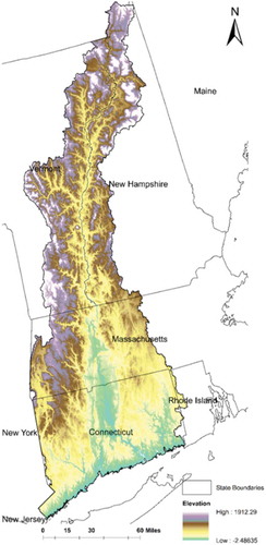
The study area is the part of the LISW within New England (Figure 1), which has an area of around 1500 square miles and accounts for 93% of the whole LISW. This region was heavily forested before the seventeenth century, but most of the land was cleared for farmlands during the eighteenth century and the early nineteenth century (Cronon 1983). As farms were abandoned, much of the land has reverted to mixed hardwood forest. By now, its surface contains more than 70% forest land. Studies showed that invasive plants tended to occur in areas with post-agricultural reforestation (DeGasperis and Motzkin 2007; Mosher, Silander, and Latimer 2009; Gavier-Pizarro et al. 2010; Parker et al. 2010). Many invasive plant species in this region were introduced during the reforestation time (around the early twentieth century) (Foster and Aber 2004; Foster et al. 2010). Non-native species and invasive woody plants have a comparative high richness in this region. For example, non-native species account for 30–35% of vascular plant species, with 3–5% of those species being considered invasive in this region (Mehrhoff 2000; Silander, Ibáñez, and Mehrhoff 2007). Recently, due to urban expansion and land use intensification, this area is facing a second phase of deforestation, which may affect the distribution of invasive species in this area.

Figure 1. Study area.

2.2. Methods

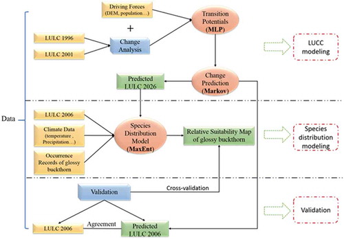
The flow chart of the study is shown in Figure 2. The LUCC drivers were identified based on literature review. The popular socio-economic and biophysical driving forces, such as elevation and population, were chosen in this study based on data availability. LULC maps in 1996 and 2001 were used to analyse how LULC has changed in the past (during the period of 1996–2001). The integrated MLP–MC model (the multi-layer perceptron [MLP] and the temporal one-dimensional Markov chain model) was used to predict how LULC will change in the future (the year of 2026). The future projection was based on the socio-economic and biophysical driving forces and the change trends in the past (during the period of 1996–2001). The predicted LULC map (for 2026), climate data and occurrence records of glossy buckthorn were then inputted into a species distribution model called MaxEnt for studying the impact of future LUCC on the spatial distribution of glossy buckthorn. MaxEnt is a technique for modelling of geographic distributions of species with presence-only data, and it has the advantage of achieving high predictive accuracy (Wisz et al. 2008; Elith and Leathwick 2009). The relative suitability was calculated for glossy buckthorn with the predicted 2026 LULC map. We also compared the calculated future relative suitability to the actual relative suitability under LULC map of 2006. The predicted 2006 land cover map and the observed 2006 land cover map were compared to validate the MLP–MC model. Cross-validation method was employed for validation of the species distribution model.

Figure 2. Flow chart of the study framework for LUCC and species distribution modelling.

2.2.1. Data

Thematically consistent LULC datasets for the years 1996, 2001 and 2006 were created by post-classification and adjustment of the original LULC maps, which were obtained from the Coastal Change Analysis Program. The adjustment was achieved by using the National Land Cover Database 1992–2001 Retrofit Land Cover Change Product (Fry et al. 2009). The datasets have a 60-m × 60-m pixel resolution and were reclassified into 14 classes for LUCC modelling. The left column of Table 1 lists the 14 classes for LUCC prediction. Based on the reclassification results, the LULC data were further simplified and aggregated to five classes for modelling the distribution of glossy buckthorn. We chose to simplify and aggregate to the five classes based on the ecological characteristics of the study species. The final simplified classes for modelling the distribution of glossy buckthorn LUCC modelling are listed in the right column of Table 1.

Table 1. Land use/cover classes.

Classes for LUCC prediction	Classes for glossy buckthorn distribution modelling
High-intensity development	Developed land
Medium-intensity development
Low-intensity development
Urban grasses	Crop/Grasses
Pastures and grasses
Crop
Scrub and shrub	Scrub/Shrub
Deciduous forest	Forest
Evergreen forest
Mixed forest
Woody wetlands
Open water	Other
Emergent wetlands
Barren land

Many important LUCC drivers were identified from the previous studies in literature (Kolb, Mas, and Galicia 2013; Bajocco et al. 2016). For example, Newman, McLaren and Wilson (2014) investigated the socio-economic drivers and biophysical drivers of LUCC in the Cockpit Country, Jamaica, and found that both of them are important factors, especially the biophysical drivers. We collected spatial data for a total of 11 explanatory variables for LUCC predicting. They include (1) biophysical drivers: elevation, slope, aspect and soil type; (2) socio-economic drivers: per capita income, population density and housing density; (3) proximity causes: distances to roads, distances to major cities, distances to water and distances to developed land. Other drivers were not applied for this study because of unavailability of data. For example, the soil erosion data are not available for the selected years, so we didn’t employ this driver. For another example, it is difficult to transfer the qualitative policy intervention data into the quantitative numerical data for the models. Therefore, we didn’t apply the policy intervention driver for the LUCC models. The majority data used in this study were derived from 2000–2002 data layers. The aspect, elevation and slope data were generated from US Geological Survey (USGS) National Elevation Dataset. The soil map, population, per capita income and housing data were downloaded from National Historical Geographic Information System. The distances to developed land were generated from the LULC map of 2001. The distances to roads were calculated in relation to primary and secondary roads, which were supplied by US Census Bureau (TIGER products). The distances to water and distances to major cities were created from water and city maps from USGS.

We compiled a database of 1027 specimen and observational records for glossy buckthorn from LISW. Specimen and field observations were obtained from the Early Detection and Distribution Mapping System, an online repository for invasive species data (EDDMapS 2016). Once downloaded, records were clipped to the study region in ArcGIS 10.3.1 (ESRI, Redlands, CA). Observations without geographic coordinates were discarded because they cannot be associated spatially with environmental data. Climate and LULC data are the main factors that determine the distribution and invasive plants at regional scales (Ficetola, Thuiller, and Miaud 2007; Petitpierre et al. 2016). Therefore, we used both climate data and the predicted future LULC data for modelling the spatial distribution of glossy buckthorn. The climate data at the 30-as scale (approximately 1 km × 1 km) were obtained from the WorldClim database (Hijmans et al. 2005). As candidate climate predictors, we reduced 19 candidate climate variables to 4 based on correlation analysis using layerStats in the raster package (Hijmans 2015) in R 3.3.1 (Team 2016) and ecological understanding of the study species. The final climate predictors included maximum temperature of the warmest month, minimum temperature of the coldest month, mean annual precipitation and precipitation seasonality. The final predictors were resampled to 60 m resolution to match the LULC data.

2.2.2. The MLP–MC LUCC model

The dynamics of future LUCC can be predicted by examining and integrating historical landscape change, social, economic, and biophysical processes using multiple approaches, such as agent-based models (Villamor et al. 2014), statistical models (Dubovyk et al. 2013), cellular automata models (Walsh et al. 2006), Markov models (Guan et al. 2011), neural network models (Shafizadeh-Moghadam et al. 2015) or combinations of these methods (Arsanjani et al. 2013). Reviews of LUCC models have been provided by Parker et al. (2003), Verburg et al. (2004) and Brown et al. (2012). In this study, the MLP–MC model combines the MLP and the temporal one-dimensional Markov chain model to predict the LUCC. The implementation of the MLP–MC model is available in IDRISI Selva (Eastman 2012a), which was developed by Clark Labs at Clark University. The prediction ability of MLP_MC has been proved in many studies (Pérez-Vega, Mas, and Ligmann-Zielinska 2012; Wang et al. 2016; Zhai et al. 2016). The functional relationships between land-cover change and driving forces were established by a MLP model, and then the Markov chain model was used to extrapolate LUCC probabilities into the future distributions of LULC types based on the established functional relationships from the MLP. The MLP model is one of the most widely used artificial neural network approaches, which have the advantage in the context of understanding land change processes (Basse et al. 2014). It can model non-linear complex land-cover patterns due to its capability of sorting patterns and learning by trials and errors.

Dynamic learning rate, starting at 0.01, was used for the MLP model in this study. Fifty percent of the dataset was used for training samples and 50% for validation. The momentum factor was set up equalling to 0.01. The sigmoid constant was given to 1. Ten-thousand iterations were conducted for training samples to obtain final accuracy rate. The training ended after reaching either an accuracy rate, or an acceptable error, or the maximum number of iterations. The model was considered acceptable when it reached an accuracy of above 75% (Eastman 2012b). At first, all the parameters of the MLP are used at their normal default values in IDRISI Selva. After several experiments for the model calibration and sensitivity analysis, we chose the best parameters for the model based on the experimental results.

The transition potential surface maps for each transition were created by MLP. The change prediction was achieved by using a Markov chain model through integrating all the transition potential surface maps with the temporal trends. The key input parameter for the Markov chain model is the transition probability matrix, which was used to describe the probabilities associated with various LULC state changes. The future LULC was predicted using the transition probability matrix P and historical LULC through an equation: =.

2.2.3. Species distribution model

Occurrence records were used in combination with climate and LULC data to develop a species distribution model for simulating the spatial distribution of glossy buckthorn in LISW. We chose the maximum entropy modelling via the software program MaxEnt (Phillips, Anderson, and Schapire 2006) because we had presence-only observations. MaxEnt is the preferred method for modelling with presence-only data due to its performance relative to alternative methods (Wisz et al. 2008; Elith and Leathwick 2009; Merow, Smith, and Silander 2013) and because it does not require selection of pseudo-absences (where the assumption is that the environments are unsuitable), but rather background points (which describes the available landscape, but does not assume unsuitability, Merow, Smith, and Silander 2013). Presence records were aggregated to the 60-m scale to match the climatic and LULC predictors for model fitting (Merow et al. 2016). The 1027 records yielded 714 observations in unique cells, once occurrence data were aggregated to the scale of the covariate data. Linear and quadratic additive features were considered to retain model interpretability (Merow, Smith, and Silander 2013) with 10-fold cross-validation and a regularization multiplier of 1 to avoid overfitting.

2.2.4. Validation

We used the three-way cross-tabulation method to measure confidence on the MLP–MC model and the 10-fold cross-validation method to measure confidence on the MaxEnt model. The three-way cross-tabulation method validated the MLP model via measuring the agreement among the LULC map of 2001, the predicted map of 2006 and the observed map of 2006. The comparison between LULC map of 2001 and the observed LULC map of 2006 reflects the observed change during the 2001–2006 period. The comparison between LULC map of 2001 and the predicted LULC map of 2006 characterizes the predicted change during the 2001–2006 period. The three-way cross-tabulation method assessed the prediction accuracy by measuring two agreements (the correctly predicted non-change and correctly predicted change) and the three disagreements (change predicted as non-change, non-change predicted as change and predicted wrong change classes). The standard Kappa index can also measure the agreement between two categorical maps. The higher the index indicates the better the agreement between them.

We used 10-fold cross-validation for validation of the species distribution model. The 10-fold cross-validation method divided the glossy buckthorn observational data into 10 folds randomly and ran the model 10 times. In each run, 90% of the glossy buckthorn observational data was used for model fitting and the remaining 10% used to compare with the prediction results for validation. Across the 10 replicate model runs, the averaged area under the receiver operating characteristic (ROC) curve (AUC) was used to evaluate the model performance based on holdout observational data (‘test AUC’; Phillips, Anderson, and Schapire 2006). AUC provides a measure of the model performance, independent of any choice of threshold. Note that ROC analysis has been used to evaluate models of species distributions in many studies (Elith 2000; Phillips and Dudík 2008).

3. Results

3.1. Transition probability

The transition from one land class to itself or another class was modelled by the MLP model. Totally, 54 plausible transitions among 14 land-cover types were modelled in this study and were divided into 9 sub-models (Table 2). From Table 2, it can be seen that the accuracy rates of most models are higher than 75%, except the sub-model 8, which has an accuracy rate slightly lower than 75%. The accuracy rates above 75% are considered acceptable (Eastman 2012b). Fifty-four transition potential maps were created and used for predicting LUCC for 2006 and 2026. Transition potential maps indicate the transition probabilities between two classes, with a range from 0 to 1. A larger transition probability means a higher possibility of change. The soft prediction map, which is a continuous map that shows the vulnerability to change for a selected set of transitions, was generated via aggregation of all the transition maps. The values of soft prediction were calculated using logical OR for all of the 54 transition potentials. The logic behind this is that a pixel will be considered to be more vulnerable if it is wanted by several transitions at the same time. For example, if a pixel has a value as its potential to transition to one land-cover type and a value to another type, then its vulnerability to change would be equal to . 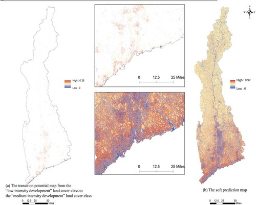A value in the soft prediction map does not mean a transition possibility, but rather a degree to which the pixel has the right condition to participate change. Figure 3(a) shows an example of a transition potential map from low-intensity development to medium-intensity development. The highest transition probability from low-intensity development to medium-intensity development is 0.26, which occurs in the pixels near coastal areas and along the Connecticut River. Figure 3(b) illustrates the soft prediction map, in which existing development areas, roads and water land have the lowest transition probability. But the pixels close to or existing development areas are more vulnerable.

Table 2. MLP sub-models and accuracy rates.

Sub-models	Description	Accuracy rate (%)
Sub-model 1	Transitions related to developed land	80.26
Sub-model 2	Transitions related to developed land	76.30
Sub-model 3	Transitions related to developed land	78.21
Sub-model 4	Transitions related to forest land	76.01
Sub-model 5	Transitions related to forest land	77.37
Sub-model 6	Transitions related to forest land	75.11
Sub-model 7	Transitions related to crop and grasses land	76.94
Sub-model 8	Transitions related to shrub land	72.56
Sub-model 9	Transitions related to other land	75.34

Figure 3. (a) The transition potential map from the ‘low-intensity development’ land use/cover class to the ‘medium-intensity development’ land use/cover class and (b) the soft prediction map.

3.2. LUCC prediction

We predicted the 2026 LULC map to illustrate possible future changes that may occur under the existing trends. A longer term simulation can provide more useful information to land planners and policy makers. So, we predicted LULC in 2026 instead of 2016. However, the complexity of LULC systems makes it difficult to predict long-term LUCC. In addition, the MLP model assumes a static process of LUCC; therefore, it has limitation on revealing temporal dynamics of LUCC. This means that with the increase of the predicted period, the reliability of the simulation results will decrease. Therefore, we chose to predict the more reliable relative short-term future (2026) LUCC instead of the long-term LUCC such as 2036. Figure 4(a,b) illustrates the observed 2006 LULC map and the predicted 2026 LULC map, respectively. From the figures, it can be seen that there is a high similarity between the projected map and the observed map. The areas and percentages of the 14 classes are shown in Table 3. One can see that the LUCC in this study area is not huge. The mean annual area changes (total change for 5 years divided by 5) of classes were also calculated from the observed maps and the predicted maps for the three time periods of 1996–2001, 2001–2006 and 2006–2026, as displayed in Table 3. There are variety scenarios to illustrate the possible LUCC under different conditions. For example, Radeloff et al. (2012) used four different scenarios, a ‘business-as-usual’ baseline scenario, an afforestation scenario, a removal of certain agricultural subsidies scenario and an increased urban land value scenario, to predict the future land use in the conterminous United States. In this paper, we used the ‘business-as-usual’ baseline scenario, which means the future change trend in this paper is assumed with no huge difference from the recent past change trend. And, these changes are allocated based on the driving factors. The annual area changes for each class are quite different between the two observed periods, 1996–2001 and 2001–2006. The annual area changes from 2001 to 2006 are generally higher than those from 1996 to 2001. The predicted change rates for the 14 classes were more similar to those in the period of 2001–2006, except that we cannot capture the changes of open water and barren land in prediction. Since open water and barren land are minor classes and their changes are small, they will not have a significant influence on the following species distribution modelling. Therefore, we considered that the prediction of 2026 LULC is reliable under the same driving forces and the historical change trend.

Table 3. The areas and percentages of 14 classes for the observed 1996, 2001, 2006 maps and the predicted 2026 map, and the mean annual area changes for the14 classes.

	1996		2001		2006		Projected 2026		Annual area change (ha)
Class	(ha)	%	(ha)	%	(ha)	%	(ha)	%	(96–01)	(01–06)	(06–26)
High-intensity development	22,697	0.57	22,953	0.57	24,118	0.60	27,385	0.69	51	233	163
Medium-intensity development	308,233	7.72	308,426	7.72	309,159	7.74	310,571	7.77	39	147	71
Low-intensity development	85,077	2.13	85,476	2.14	85,497	2.14	87,117	2.18	80	4	81
Urban grasses	101,476	2.54	101,552	2.54	102,192	2.56	103,865	2.60	15	128	84
Pastures and grasses	235,680	5.90	236,476	5.92	240,668	6.02	256,715	6.42	159	838	802
Crop	66,147	1.66	66,548	1.67	67,274	1.68	69,031	1.73	80	145	88
Scrub and shrub	71,326	1.78	76,536	1.92	81,241	2.03	100,286	2.51	1042	941	952
Deciduous forest	1633,014	40.86	1627,911	40.74	1620,306	40.55	1592,086	39.84	−1021	−1521	−1411
Evergreen forest	533,970	13.36	532,341	13.32	530,132	13.27	522,642	13.08	−326	−442	−375
Mixed forest	640,083	16.01	639,042	15.99	636,392	15.92	626,921	15.69	−208	−530	−474
Woody wetlands	111,501	2.79	111,555	2.79	111,429	2.79	166,132	4.16	−5	−73	−60
Open water	11,757	0.29	11,748	0.29	12,012	0.30	111,429	2.79	11	−25	0
Emergent wetlands	167,721	4.20	167,694	4.20	167,328	4.19	13,567	0.34	−2	53	78
Barren land	7610	0.19	8032	0.20	8544	0.21	8544	0.21	85	102	0

Figure 4. (a) The observed 2006 land use/cover map. (b) The projected 2026 land use/cover map.

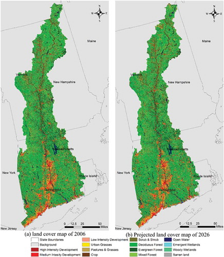
Table 3 shows that the major land-cover/use class in LISW is forest land, especially deciduous forest. In general, there was an increase in all kinds of developed land, grasses, crops and scrub/shrub, and a decrease in forest land over the two 5-year periods of 1996–2001 and 2001–2006. Approximately 7773 ha of forest was lost within the period 1996–2001, while almost twice that area, 12,465 ha of forest, was lost within the period 1996–2006. At the same time, the total area of developed land had an increase of 848 ha during 1996–2001 and its increase was 1919 ha during 2001–2006. It appears that there was an increasing trend of losing forest area and an increasing trend of adding developed area.

3.3. Species distribution modelling results

The observed 2006 LULC map and the predicted 2026 LULC map were used as inputs in our species distribution model. The MaxEnt model exhibits additivity with the contributions of all the variables being added at each pixel. And, the average percentage contribution of each predictor variable to the model (‘percentage contribution’; Phillips, Anderson, and Schapire 2006) was used to assess the importance of each variable to the model. Our species distribution model showed that precipitation seasonality and the minimum temperature of the coldest month were the primary drivers to the distribution of glossy buckthorn in the study region, followed by the maximum temperature of the warmest month and LULC (Table 4). Of the LULC variables, developed land (its mean relative suitability is 4.13 × 10⁻⁴) had the largest effect on relative suitability compared to forests (mean relative suitability 2.0 × 10⁻⁴), scrub/shrub (mean relative suitability 2.5 × 10⁻⁴) and crop/grassland (mean relative suitability 2.6 × 10⁻⁴).

Table 4. Percentage contributions of predictors to the species distribution model of glossy buckthorn in Long Island Sound Watersheds.

Predictor	Percentage contribution
Precipitation seasonality	36.7
Minimum temperature of the coldest month	30.0
Maximum temperature of the warmest month	19.5
Land use/cover	11.7
Mean annual precipitation	2.2

To calculate the effect of LUCCs by 2026, we applied the thresholds to the continuous relative suitability output. We chose the threshold that encompassed 95% of the model training points in each model replicate and then averaged the threshold identified across 10 replicate model runs. The averaged 95% minimum training presence threshold represents a compromise to characterize the species’ full potential distribution while guarding against outlier observations (Allen and Bradley 2016; Bocsi et al. 2016). We calculated the range sizes of glossy buckthorn with the observed 2006 and the predicted 2026 LULC to estimate the effect of landscape changes on range size.

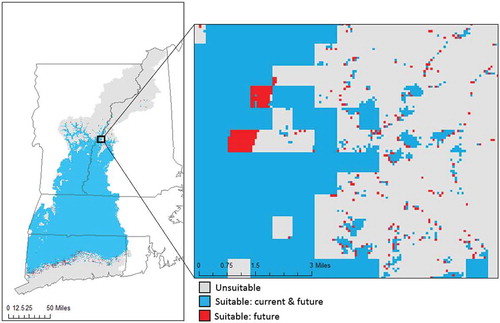
The maps of modelled relative suitability for glossy buckthorn suggest that the potential distribution in 2026 will be slightly different from that in 2006 (Figures 5 and 6). For example, the core area of the potential distribution of glossy buckthorn in 2026 remains to be in the centre of the study region, but the suitability in some small pockets of formerly moderate suitability, such as those in the southwest portion of the study region, will increase. Nearly all known occurrence points in our dataset fall within the areas with modelled high relative suitability (Figure 5). When the two suitability maps for 2006 and 2026 were transformed into binary data using a 95% minimum training presence threshold, the suitable area for glossy buckthorn was found to increase by 0.18% (5578,200 m²) by 2026 due to LUCC (Figure 6).

Figure 5. Relative suitability predictions for glossy buckthorn with the observed 2006 (a) and the predicted 2026 (b) land use/cover maps in Long Island Sound Watersheds. Black points indicate the known occurrence locations of glossy buckthorn.

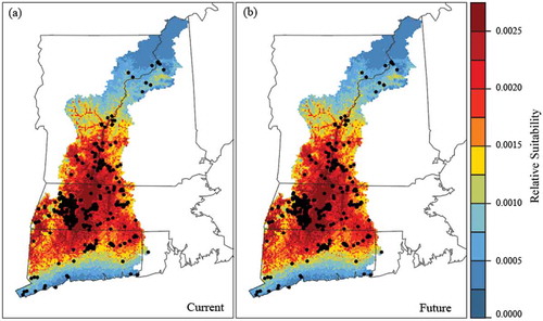
Figure 6. Modelled suitability map for glossy buckthorn with the observed current (2006) land use/cover map and the predicted future (2026) land use/cover map.

3.4. Validation results

Based on the three-way cross-tabulation of the observed and the predicted LUCCs, the five categories (i.e. observed non-change–predicted non-change, observed change–predicted change, observed change–predicted non-change, observed non-change–predicted change and observed change–predicted change but to the wrong class) were estimated, shown in Table 5. In these five categories, observed non-change–predicted non-change and observed change–predicted change are the agreement categories between the observed and the predicted LULC maps of 2006 compared to the observed 2001 map. The total agreement is the sum of areas of the two agreed categories divided by the total area. The agreement of non-change is the ratio of the non-changed area that had been correctly predicted to the amount of the non-changed area; similarly, the agreement of change is the ratio of the changed area that had been correctly predicted to the amount of the changed area. The rest are the three disagreement categories between them. Percentage in total area is the area of each category divided by the total research area. From Table 5, it can be seen that the amount of non-predicted change area (under-prediction), 18,117 ha, is close to the amount of non-predicted non-change area (over-prediction), 15,102 ha. The agreement of non-change is 99.62%, while the agreement of change is 33.50%; the former is three times of the latter. In general, the overall agreement between the observed and the predicted LUCC is 99.15% and the Kappa index is 0.986. For presence-only data, the maximum achievable AUC is less than 1 (Wiley et al. 2003), and the random prediction has an AUC of 0.5. After 10 replicate distribution model runs, in this study, we received an averaged AUC of 0.809 for the distribution model, with a standard deviation of 0.027.

Table 5. Areas and percentages of different categories of agreement/disagreement between the observed 2006 and the predicted 2006 land use/cover maps.

Observed–predicted	Area (ha)	Percentage of total area (%)	Agreement (%)
Non-change–non-change	3953,020	98.92	99.62
Change–change	9436	0.24	33.50
Change–non-change	18,117	0.45
Non-change–change	15,102	0.38
Wrong change	617	0.02
Total agreement	99.15%
Kappa	0.986

4. Discussions

4.1. LUCC

This study indicates that the loss of forest land and increase of developed land happened during 1996–2006. The loss of forest is small, as it only accounts for 0.5% of the total area; however, it is huge when we look at the lost area, 20,238 ha, in the period. Most of the lost forest was transferred to scrub and shrub land. This transition was linked with urban growth, especially suburbanization, because urban growth pushed the urban edge further and consequently promoted the increase of fragmentation and forest degradation. Some studies found similar results. For example, Brown et al. (2005) stated that there was a large increase in the area of low-density, exurban development during 1950–2000 across the conterminous United States, especially in the eastern United States. Jeon, Olofsson and Woodcock (2014) indicated that the New England was facing a secondary phase of forest transition. They found that the loss of forest was driven by the increase of residential and commercial development in suburban areas, instead of agricultural expansion.

Our prediction shows that the decrease of forest land and increase of developed land will continue and alter the suitability of the region for glossy buckthorn. Our simulated transition potential maps show that high transition probability for the conversion from forest to scrub/shrub occurs at forest edge and in areas close to roads; and the high transition probabilities from scrub/shrub, grass, crop and forest to developed land of varying intensities occur in areas that are close to roads, existing urban areas, coastal areas and the Connecticut River. Our prediction reveals that the largest annual area changes are the decrease in deciduous forest and the increase in scrub/shrub, implying that conversion from forest to scrub/shrub will be the dominant future LUCC expected in the study region.

4.2. Model validation and uncertainty

LUCC is a complex process, which cannot be simply modelled. The overall agreement between our prediction and the observed data is high, mainly because the prediction accuracy of non-changed area is high and the percentage of changed area in the whole study area is small. The prediction accuracy of non-changed area is more than three times of the prediction accuracy of changed area. This indicates that our model has a better performance in predicting the non-changed area. The prediction of changed area is more difficult, because it is affected by many driver forces. At the same time, the amount of over-prediction (non-change by observation–change by prediction) is similar to the amount of under-prediction (change by observation–non-change by prediction); thus, the predicted total changed area is close to the actual total changed area. The validation results of our LUCC model and the species distribution model proved that both models are reliable. However, there are limitations of the applied models in this study. For example, the MLP model used a ‘black-box’ process, which makes modification of the relationships between the explanatory variables and LUCC results difficult. Although we conducted the model calibration and sensitivity analysis and we chose the best parameters for the models, the uncertainties that related to model parameters and model structures still need to be studied further.

4.3. Glossy buckthorn responses to landscape change

The predicted changes in relative suitability for glossy buckthorn from 2006 to 2026 are driven by LUCC. The developed land class is the most important driver among the LULC classes in increasing the relative suitability in LISW for glossy buckthorn, which reflects the close relationship between anthropogenic disturbance and the presence of the glossy buckthorn. According to our prediction, the developed land class will keep increasing by 2026 as the development pressure continues. Similarly, scrub/shrub land and crop/grass land, the secondarily influential LULC classes for glossy buckthorn occurrence, will also have an increase by 2026. These classes are also related to human management of the landscape and are likely to have higher disturbance than the forest class to the local ecosystems. These explain the projected increase in glossy buckthorn suitability in the study area. The linkage between disturbance and invasive plant occurrence holds for other similar species in the north-eastern United States (Allen et al. 2013), so the changes observed and predicted here are likely indicative of broader establishment opportunities for invasive plants in LISW.

This study used the predicted future LULC data as input into a species distribution model to simulate the future range size of glossy buckthorn in the LISW. The MLP model is a general-purpose model and has been used in many studies at a variety of locations and different time ranges (Ozturk 2015; Losiri et al. 2016). The MaxEnt model was used for modelling the species distribution because it can consistently perform well for predictions of presence-only data (Syfert, Smith, and Coomes 2013). The coupling of these two models is a general-purpose method. The method is not location specific and can be broadly applicable for research problems at different locations and scales (spatial and temporal). However, the prediction accuracy of the method may depend on other factors behind this method, such as the accuracy of the input data.

5. Conclusions

Although many studies have been conducted to explore the effect of historical LUCC on species in literature, there are few studies to predict the possible effect of future LUCC on species. This paper combines two simulation models, a LUCC model and a species distribution model, to study the future LUCC and its effect on the distribution of invasive plants (taking the glossy buckthorn as an example) in LISW. LUCC modelling can only present an approximate representation of the future LULC situation. The prediction is achieved by analysing the past change trend and establishing the functional relationships between LUCC and driving forces, which include both socio-economic and biophysical factors. Due to the fact that the input driving forces lack dynamic information, when we extended the prediction into a future date, the uncertainty of the result could increase.

Even though the LUCC prediction only presents an approximate representation of the future, it is still an effective tool in understanding the processes of LUCC. Furthermore, the prediction can inform land planners, policy maker and natural resource managers of the effect of LUCC may have on biodiversity and ecosystem function. Our prediction indicates that the suitable area for glossy buckthorn will increase 558 ha by 2026 due to LUCC, which will affect the growth of native plants.

Future LUCC may affect ecological systems in many ways. Here, we provide one example – its effect on the spatial distribution of one invasive plant, glossy buckthorn. Since the study region will undergo a rapid LUCC, the resource managers and other related governmental agencies should pay attention to its future effect on biodiversity and ecological systems, such as the richness of invasive plants and the stability of forest services. The improvement of the research approach and its further application to other species could help to deepen our understanding of the future LUCC effect on the distribution of species and help to improve the management of ecosystems.

Disclosure statement

No potential conflict of interest was reported by the authors.

Additional information

Funding

This work was supported by the United States NSF: [Grant Number 1414108].

References

- Allen, J. M., and B. A. Bradley. 2016. “Out of the Weeds? Reduced Plant Invasion Risk with Climate Change in the Continental United States.” Biological Conservation 203: 306–312. doi:10.1016/j.biocon.2016.09.015.
- Allen, J. M., T. J. Leininger, J. D. Hurd, D. L. Civco, A. E. Gelfand, and J. A. Silander. 2013. “Socioeconomics Drive Woody Invasive Plant Richness in New England, USA through Forest Fragmentation.” Landscape Ecology 28 (9): 1671–1686. doi:10.1007/s10980-013-9916-7.
- Arsanjani, J. J., M. Helbich, W. Kainz, and A. D. Boloorani. 2013. “Integration of Logistic Regression, Markov Chain and Cellular Automata Models to Simulate Urban Expansion.” International Journal of Applied Earth Observation and Geoinformation 21: 265–275. doi:10.1016/j.jag.2011.12.014.
- Bajocco, S., T. Ceccarelli, D. Smiraglia, L. Salvati, and C. Ricotta. 2016. “Modeling the Ecological Niche of Long-Term Land Use Changes: The Role of Biophysical Factors.” Ecological Indicators 60: 231–236. doi:10.1016/j.ecolind.2015.06.034.
- Basse, R. M., H. Omrani, O. Charif, P. Gerber, and K. Bódis. 2014. ““Land Use Changes Modelling Using Advanced Methods: Cellular Automata and Artificial Neural Networks. The Spatial and Explicit Representation of Land Cover Dynamics at the Cross-Border Region Scale.” Applied Geography 53: 160–171. doi:10.1016/j.apgeog.2014.06.016.
- Bocsi, T., J. M. Allen, J. Bellemare, J. Kartesz, M. Nishino, and B. A. Bradley. 2016. “Plants’ Native Distributions Do Not Reflect Climatic Tolerance.”.” Diversity and Distributions. doi:10.1111/ddi.12432.
- Brown, D. G., K. M. Johnson, T. R. Loveland, and D. M. Theobald. 2005. “Rural Land‐Use Trends In The Conterminous United States, 1950–2000.” Ecological Applications 15 (6): 1851–1863. doi:10.1890/03-5220.
- Brown, D. G., R. Walker, S. Manson, and K. Seto. 2012. “Modeling Land Use and Land Cover Change.” In Land Change Science. Remote Sensing and Digital Image Processing, Vol. 6, edited by G. Gutman et al. Dordrecht: Springer.
- Cousins, S. A., A. G. Auffret, J. Lindgren, and L. Tränk. 2015. “Regional-Scale Land-Cover Change during the 20th Century and Its Consequences for Biodiversity.” Ambio 44 (1): 17–27. doi:10.1007/s13280-014-0585-9.
- Cronon, W. 1983. Changes in the Land: Indians, Colonists, and the Ecology of New England. New York: Hill and Wang.
- Cunard, C., and T. D. Lee. 2009. “Is Patience a Virtue? Succession, Light, and the Death of Invasive Glossy Buckthorn (Frangula Alnus).” Biological Invasions 11 (3): 577–586. doi:10.1007/s10530-008-9272-8.
- Cusser, S., J. L. Neff, and S. Jha. 2016. “Natural Land Cover Drives Pollinator Abundance and Richness, Leading to Reductions in Pollen Limitation in Cotton Agroecosystems.”.” Agriculture, Ecosystems & Environment 226: 33–42. doi:10.1016/j.agee.2016.04.020.
- De Chazal, J., and M. D. Rounsevell. 2009. “Land-Use and Climate Change within Assessments of Biodiversity Change: A Review.” Global Environmental Change 19 (2): 306–315. doi:10.1016/j.gloenvcha.2008.09.007.
- DeGasperis, B. G., and G. Motzkin. 2007. “Windows of Opportunity: Historical and Ecological Controls on Berberis Thunbergii Invasions.” Ecology 88 (12): 3115–3125. doi:10.1890/06-2014.1.
- Dubovyk, O., G. Menz, C. Conrad, E. Kan, M. Machwitz, and A. Khamzina. 2013. “Spatio-Temporal Analyses of Cropland Degradation in the Irrigated Lowlands of Uzbekistan Using Remote-Sensing and Logistic Regression Modeling.” Environmental Monitoring and Assessment 185 (6): 4775–4790. doi:10.1007/s10661-012-2904-6.
- Eastman, J. 2012a. IDRISI Selva–GIS and Image Processing Software–Version 17.0. Worcester: Clark Labs.
- Eastman, J. R. 2012b. IDRISI Selva Tutorial, 51–63. Vol. 45. Idrisi Production, Clark Labs-Clark University. Accessed 10 March 2018. http://uhulag.mendelu.cz/files/pagesdata/eng/gis/idrisi_selva_tutorial.pdf
- EDDMapS. 2016. “Early Detection and Distribution Mapping System.” https://www.eddmaps.org/.
- Elith, J. 2000. “Quantitative Methods for Modeling Species Habitat: Comparative Performance and an Application to Australian Plants.” In Quantitative Methods for Conservation Biology, edited by S. Ferson and M. Burgman, 39-58. New York: Springer-Verlag.
- Elith, J., and J. R. Leathwick. 2009. “Species Distribution Models: Ecological Explanation and Prediction across Space and Time.”.” Annual Review of Ecology, Evolution, and Systematics 40: 677–697. doi:10.1146/annurev.ecolsys.110308.120159.
- Emerton, L., and G. Howard. 2008. A Toolkit for the Economic Analysis of Invasive Species. Nairobi: Global Invasive Species Programme.
- Fagan, M., and D. Peart. 2004. “Impact of the Invasive Shrub Glossy Buckthorn (Rhamnus Frangula L.) On Juvenile Recruitment by Canopy Trees.” Forest Ecology and Management 194 (1): 95–107. doi:10.1016/j.foreco.2004.02.015.
- Ficetola, G. F., W. Thuiller, and C. Miaud. 2007. “Prediction and Validation of the Potential Global Distribution of a Problematic Alien Invasive Species—The American Bullfrog.” Diversity and Distributions 13 (4): 476–485. doi:10.1111/j.1472-4642.2007.00377.x.
- Foster, D., J. Aber, C. Cogbill, C. Hart, E. Colburn, A. D’Amato, B. Donahue, et al. 2010. Wildlands and Woodlands: A Vision for the New England Landscape. Cambridge, MA: Harvard Forest; Harvard University Press.
- Foster, D. R., and J. Aber, editors. 2004. “Forests in Time. Ecosystem Structure and Function as a Consequence of 1000 Years of Change.” In Synthesis Volume of the Harvard Forest LTER Program. New Haven, CT: Yale University Press.
- Frappier, B., R. T. Eckert, and T. D. Lee. 2004. “Experimental Removal of the Non-Indigenous Shrub Rhamnus Frangula (Glossy Buckthorn): Effects on Native Herbs and Woody Seedlings.” Northeastern Naturalist 11 (3): 333–342. doi:10.1656/1092-6194(2004)011[0333:EROTNS]2.0.CO;2.
- Fry, J. A., M. J. Coan, C. G. Homer, D. K. Meyer, and J. D. Wickham. 2009. Completion of the National Land Cover Database (NLCD) 1992-2001 Land Cover Change Retrofit product: U.S. Geological Survey Open-File Report 2008-1379, 18 p.
- Gavier-Pizarro, G. I., V. C. Radeloff, S. I. Stewart, C. D. Huebner, and N. S. Keuler. 2010. “Housing Is Positively Associated with Invasive Exotic Plant Species Richness in New England, USA.” Ecological Applications 20 (7): 1913–1925. doi:10.1890/09-2168.1.
- Guan, D., H. Li, T. Inohae, W. Su, T. Nagaie, and K. Hokao. 2011. “Modeling Urban Land Use Change by the Integration of Cellular Automaton and Markov Model.” Ecological Modelling 222 (20): 3761–3772. doi:10.1016/j.ecolmodel.2011.09.009.
- Hepinstall, J. A., M. Alberti, and J. M. Marzluff. 2008. “Predicting Land Cover Change and Avian Community Responses in Rapidly Urbanizing Environments.” Landscape Ecology 23 (10): 1257–1276. doi:10.1007/s10980-008-9296-6.
- Hijmans, R. 2015. “Raster: Geographic Data Analysis and Modeling. R Package Version 2.3-24.” Accessed 10 March 2018. http://CRAN.R-project.org/package=raster.
- Hijmans, R. J., S. E. Cameron, J. L. Parra, P. G. Jones, and A. Jarvis. 2005. “Very High Resolution Interpolated Climate Surfaces for Global Land Areas.” International Journal of Climatology 25 (15): 1965–1978. doi:10.1002/(ISSN)1097-0088.
- Hobbs, T. J., C. R. Neumann, W. S. Meyer, T. Moon, and B. A. Bryan. 2016. “Models of Reforestation Productivity and Carbon Sequestration for Land Use and Climate Change Adaptation Planning in South Australia.” Journal of Environmental Management 181: 279–288. doi:10.1016/j.jenvman.2016.06.049.
- Ibáñez, I., J. A. Silander, A. M. Wilson, N. LaFleur, N. Tanaka, and I. Tsuyama. 2009. “Multivariate Forecasts of Potential Distributions of Invasive Plant Species.” Ecological Applications 19 (2): 359–375. doi:10.1890/07-2095.1.
- Jeon, S. B., P. Olofsson, and C. E. Woodcock. 2014. “Land Use Change in New England: A Reversal of the Forest Transition.” Journal of Land Use Science 9 (1): 105–130. doi:10.1080/1747423X.2012.754962.
- Jetz, W., D. S. Wilcove, and A. P. Dobson. 2007. “Projected Impacts of Climate and Land-Use Change on the Global Diversity of Birds.” PLoS Biol 5 (6): e157. doi:10.1371/journal.pbio.0050157.
- Kolb, M., J.-F. Mas, and L. Galicia. 2013. “Evaluating Drivers of Land-Use Change and Transition Potential Models in a Complex Landscape in Southern Mexico.” International Journal of Geographical Information Science 27 (9): 1804–1827. doi:10.1080/13658816.2013.770517.
- Koning, C. O., and R. Singleton. 2013. “Effects of Moderate Densities of Glossy Buckthorn on Forested Plant Communities in Southwest New Hampshire, USA.” Natural Areas Journal 33 (3): 256–263. doi:10.3375/043.033.0304.
- Losiri, C., M. Nagai, S. Ninsawat, and R. P. Shrestha. 2016. “Modeling Urban Expansion in Bangkok Metropolitan Region Using Demographic–Economic Data through Cellular automata-Markov Chain and multi-Layer perceptron-Markov Chain Models.” Sustainability 8 (7): 686. doi:10.3390/su8070686.
- Mantyka-Pringle, C. S., P. Visconti, M. Di Marco, T. G. Martin, C. Rondinini, and J. R. Rhodes. 2015. “Climate Change Modifies Risk of Global Biodiversity Loss Due to Land-Cover Change.” Biological Conservation 187: 103–111. doi:10.1016/j.biocon.2015.04.016.
- Marzluff, J. M. 2008. “Island Biogeography for an Urbanizing World How Extinction and Colonization May Determine Biological Diversity in Human-Dominated Landscapes.” In Urban Ecology, edited by J. M. Marzluff. Boston, MA: Springer.
- Mehrhoff, L. J. 2000. “Immigration and Expansion of the New England Flora.” Rhodora 102: 280–298.
- Merow, C., J. M. Allen, M. Aiello‐Lammens, and J. A. Silander. 2016. “Improving Niche and Range Estimates with Maxent and Point Process Models by Integrating Spatially Explicit Information.” Global Ecology and Biogeography 25 (8): 1022–1036. doi:10.1111/geb.12453.
- Merow, C., M. J. Smith, and J. A. Silander. 2013. “A Practical Guide to MaxEnt for Modeling Species’ Distributions: What It Does, and Why Inputs and Settings Matter.” Ecography 36 (10): 1058–1069. doi:10.1111/ecog.2013.36.issue-10.
- Mosher, E. S., J. A. Silander Jr, and A. M. Latimer. 2009. “The Role of Land-Use History in Major Invasions by Woody Plant Species in the Northeastern North American Landscape.” Biological Invasions 11 (10): 2317–2328. doi:10.1007/s10530-008-9418-8.
- Newman, M. E., K. P. McLaren, and B. S. Wilson. 2014. “Long-Term Socio-Economic and Spatial Pattern Drivers of Land Cover Change in a Caribbean Tropical Moist Forest, the Cockpit Country, Jamaica.” Agriculture, Ecosystems & Environment 186: 185–200. doi:10.1016/j.agee.2014.01.030.
- Ozturk, D. 2015. “Urban Growth Simulation of Atakum (Samsun, Turkey) Using Cellular automata-Markov Chain and Multi-Layer Perceptron-Markov Chain Models.” Remote Sensing 7 (5): 5918–5950. doi:10.3390/rs70505918.
- Padilla, F. M., B. Vidal, J. Sánchez, and F. I. Pugnaire. 2010. “Land-Use Changes and Carbon Sequestration through the Twentieth Century in a Mediterranean Mountain Ecosystem: Implications for Land Management.” Journal of Environmental Management 91 (12): 2688–2695. doi:10.1016/j.jenvman.2010.07.031.
- Parker, D. C., S. M. Manson, M. A. Janssen, M. J. Hoffmann, and P. Deadman. 2003. “Multi-Agent Systems for the Simulation of Land-Use and Land-Cover Change: A Review.” Annals of the Association of American Geographers 93 (2): 314–337. doi:10.1111/1467-8306.9302004.
- Parker, J. D., L. J. Richie, E. M. Lind, and K. O. Maloney. 2010. “Land Use History Alters the Relationship between Native and Exotic Plants: The Rich Don’t Always Get Richer.” Biological Invasions 12 (6): 1557–1571. doi:10.1007/s10530-009-9568-3.
- Paul, M. J., and J. L. Meyer. 2001. “Streams in the Urban Landscape.” Annual Review of Ecology and Systematics 333–365. doi:10.1146/annurev.ecolsys.32.081501.114040.
- Pérez-Vega, A., J.-F. Mas, and A. Ligmann-Zielinska. 2012. “Comparing Two Approaches to Land Use/Cover Change Modeling and Their Implications for the Assessment of Biodiversity Loss in a Deciduous Tropical Forest.” Environmental Modelling & Software 29 (1): 11–23. doi:10.1016/j.envsoft.2011.09.011.
- Petitpierre, B., K. McDougall, T. Seipel, O. Broennimann, A. Guisan, and C. Kueffer. 2016. “Will Climate Change Increase the Risk of Plant Invasions into Mountains?” Ecological Applications 26 (2): 530–544. doi:10.1890/14-1871.
- Phillips, S. J., R. P. Anderson, and R. E. Schapire. 2006. “Maximum Entropy Modeling of Species Geographic Distributions.” Ecological Modelling 190 (3): 231–259. doi:10.1016/j.ecolmodel.2005.03.026.
- Phillips, S. J., and M. Dudík. 2008. “Modeling of Species Distributions with Maxent: New Extensions and a Comprehensive Evaluation.” Ecography 31 (2): 161–175. doi:10.1111/j.0906-7590.2008.5203.x.
- Polasky, S., E. Nelson, D. Pennington, and K. A. Johnson. 2011. “The Impact of Land-Use Change on Ecosystem Services, Biodiversity and Returns to Landowners: A Case Study in the State of Minnesota.” Environmental and Resource Economics 48 (2): 219–242. doi:10.1007/s10640-010-9407-0.
- Radeloff, V. C., E. Nelson, A. J. Plantinga, D. J. Lewis, D. Helmers, J. J. Lawler, J. C. Withey, et al. 2012. “Economic-Based Projections of Future Land Use in the Conterminous United States under Alternative Policy Scenarios.” Ecological Applications 22 (3): 1036–1049. doi:10.1890/11-0306.1.
- Ricketts, T. H., J. Regetz, I. Steffan‐Dewenter, S. A. Cunningham, C. Kremen, A. Bogdanski, B. Gemmill‐Herren, S. S. Greenleaf, A. M. Klein, and M. M. Mayfield. 2008. “Landscape Effects on Crop Pollination Services: Are There General Patterns?” Ecology Letters 11 (5): 499–515. doi:10.1111/j.1461-0248.2008.01157.x.
- Sala, O. E., F. S. Chapin, J. J. Armesto, E. Berlow, J. Bloomfield, R. Dirzo, E. Huber-Sanwald, L. F. Huenneke, R. B. Jackson, and A. Kinzig. 2000. “Global Biodiversity Scenarios for the Year 2100.” Science 287 (5459): 1770–1774. doi:10.1126/science.287.5459.1770.
- Sanford, N. L., R. A. Harrington, and J. H. Fownes. 2003. “Survival and Growth of Native and Alien Woody Seedlings in Open and Understory Environments.” Forest Ecology and Management 183 (1): 377–385. doi:10.1016/S0378-1127(03)00141-5.
- Schulp, C. J., G.-J. Nabuurs, and P. H. Verburg. 2008. “Future Carbon Sequestration in Europe—Effects of Land Use Change.” Agriculture, Ecosystems & Environment 127 (3): 251–264. doi:10.1016/j.agee.2008.04.010.
- Shafizadeh-Moghadam, H., J. Hagenauer, M. Farajzadeh, and M. Helbich. 2015. “Performance Analysis of Radial Basis Function Networks and Multi-Layer Perceptron Networks in Modeling Urban Change: A Case Study.” International Journal of Geographical Information Science 29 (4): 606–623. doi:10.1080/13658816.2014.993989.
- Silander, J. A., I. Ibáñez, and L. Mehrhoff. 2007. “The Biology and Ecology of Invasive Species – The Importance of International Collaboration in Predicting the Spread of Invasive Species.” Proceedings of the NIAES International Symposium. NIAES International Symposium, Tsukuba, 8–17.
- Syfert, M. M., M. J. Smith, and D. A. Coomes. 2013. “The Effects of Sampling Bias and Model Complexity on the Predictive Performance of MaxEnt Species Distribution Models.” PloS One 8 (2): e55158. doi:10.1371/journal.pone.0055158.
- Team, R. C. 2016. R: A Language and Environment for Statistical Computing. Vienna: R Foundation for Statistical Computing. 2014.
- USDA. 2016. “The PLANTS Database.” http://plants.usda.gov.
- Verburg, P. H., P. P. Schot, M. J. Dijst, and A. Veldkamp. 2004. “Land Use Change Modelling: Current Practice and Research Priorities.” GeoJournal 61 (4): 309–324. doi:10.1007/s10708-004-4946-y.
- Vila, M., and I. Ibáñez. 2011. “Plant Invasions in the Landscape.” Landscape Ecology 26 (4): 461–472. doi:10.1007/s10980-011-9585-3.
- Villamor, G. B., Q. B. Le, U. Djanibekov, M. Van Noordwijk, and P. L. Vlek. 2014. “Biodiversity in Rubber Agroforests, Carbon Emissions, and Rural Livelihoods: An Agent-Based Model of Land-Use Dynamics in Lowland Sumatra.” Environmental Modelling & Software 61: 151–165. doi:10.1016/j.envsoft.2014.07.013.
- Walsh, S. J., B. Entwisle, R. R. Rindfuss, and P. H. Page. 2006. “Spatial Simulation Modelling of Land Use/Land Cover Change Scenarios in Northeastern Thailand: A Cellular Automata Approach.” Journal of Land Use Science 1 (1): 5–28. doi:10.1080/17474230600604213.
- Wang, W., C. Zhang, J. M. Allen, W. Li, M. A. Boyer, K. Segerson, and J. A. Silander. 2016. “Analysis and Prediction of Land Use Changes Related to Invasive Species and Major Driving Forces in the State of Connecticut.” Land 5 (3): 25. doi:10.3390/land5030025.
- Webster, C. R., M. A. Jenkins, and S. Jose. 2006. “Woody Invaders and the Challenges They Pose to Forest Ecosystems in the Eastern United States.” Journal of Forestry 104 (7): 366–374.
- Wiley, E. O., K. M. McNyset, A. T. Peterson, C. R. Robins, and A. M. Stewart. 2003. “Niche Modeling Perspective on Geographic Range Predictions in the Marine Environment Using a Machine-Learning Algorithm.” Oceanography 16: 120–127. doi:10.5670/oceanog.
- Wimberly, M. C., and J. L. Ohmann. 2004. “A Multi-Scale Assessment of Human and Environmental Constraints on Forest Land Cover Change on the Oregon (USA) Coast Range.” Landscape Ecology 19 (6): 631–646. doi:10.1023/B:LAND.0000042904.42355.f3.
- Wisz, M. S., R. Hijmans, J. Li, A. T. Peterson, C. Graham, and A. Guisan. 2008. “Effects of Sample Size on the Performance of Species Distribution Models.” Diversity and Distributions 14 (5): 763–773. doi:10.1111/ddi.2008.14.issue-5.
- Zhai, R., C. Zhang, W. Li, M. Boyer, and D. Hanink. 2016. “Prediction of Land Use Change in Long Island Sound Watersheds Using Nighttime Light Data.” Land 5 (4): 44. doi:10.3390/land5040044.