A near real-time flood-mapping approach by integrating social media and post-event satellite imagery

ABSTRACT

Rapid flood mapping is critical for timely damage assessment and post-event recovery support. Remote sensing provides spatially explicit information for the mapping process, but its real-time imagery is often not available due to bad weather conditions during the event. Using the 2015 South Carolina Flood in downtown Columbia as a case study, this article proposes a novel approach to retrieve near real-time flood probability map by integrating the post-event remote sensing data with the real-time volunteered geographic information (VGI). Relying on each VGI point, an inverse distance weighted height filter was introduced to build a probability index distribution (PID) layer from the high-resolution digital elevation model (DEM) data. For each PID layer, a Gaussian kernel was developed to extract its moisture weight from the normalized difference water index (NDWI) of an EO-1 Advanced Land Imager (ALI) image. Finally, a normalized flood probability map was produced by chaining the moisture weighted PIDs in a Python environment. Results indicate that, by adding the wetness information from post-event satellite observations, the proposed model could provide near real-time flood probability distribution with real-time social media, which is of great importance for emergency responders to quickly identify areas in need of immediate attention.

KEYWORDS:

• NDWI
• rapid flood mapping
• remote sensing
• tweets
• volunteered geographic information

Introduction

Flood is one of the most common natural hazards on terrestrial lands. A flood often occurs as an overflow of water from water bodies like lakes and rivers during extreme weather events (Ashley and Ashley 2008). Globally, one-third of the annual natural disasters and economic losses and more than half of victims are flood-induced (Douben 2006). Floods also cast long-term impacts via indirect damages such as human health, personal properties, public infrastructure, water quality, and ecosystems (Messner and Meyer 2006; Adhikari et al. 2010).

Flood assessment is able to reconstruct the damage zone and evaluate the losses, rendering valuable suggestions for policy makers (Rasid, Haider, and Hunt 2000; Kulkarni et al. 2014). Flood mapping, an important aspect of flood assessment, provides better situation awareness for the public and quickly draws attention to certain areas where immediate actions are needed. Numerous studies have been conducted to generate flood inundation maps for emergency responders, which could roughly break into two categories: hydrological modeling (Yin et al. 2015; Chen, Hill, and Urbano 2009; Stefanidis and Stathis 2013; Di Baldassarre et al. 2010) and remote sensing (Qiao et al. 2012; Palacios-Orueta et al. 2006).

Hydrological modeling for flood mapping (mostly for prediction purposes) has witnessed up-surging interests in past decades. However, it has always been criticized to be site specific, which requires detailed landscape-based inputs and careful parametric calibration (Efstratiadis and Koutsoyiannis 2010). In addition, their results are greatly dependent on spatial scales and land-use/cover characteristics, which increase the model uncertainties and make them difficult to be generalized (Blöschl and Sivapalan 1995; Renard et al. 2010).

Remote sensing has long been used to monitor flood coverage and its dynamic development. A variety of approaches have been developed for deriving rainfall (Villarini et al. 2010), acquiring soil wetness and soil saturation (Njoku and Entekhabi 1996), mapping potential inundation areas (Townsend and Walsh 1998), and assessing flood damage (Van Der Sande, De Jong, and De Roo 2003). Multispectral images have been utilized for extracting the characteristics of hydrological surfaces, including topography, soil saturation status, and delineation of flooding zones (Tralli et al. 2005; Davranche, Poulin, and Lefebvre 2013). As an example of spectral ratioing of multispectral images, the normalized difference water index (NDWI) has been extensively used as an indicator of soil wetness and an effective approach to delineating water boundaries and flood-prone areas (Mallinis et al. 2013; Ho, Umitsu, and Yamaguchi 2010; Jain et al. 2005; McFeeters 1996). The NDWI is a widely used water index calculated as a spectral ratio between green and shortwave-infrared (SWIR) bands (Gao 1996). However, limited temporal resolution due to a satellite’s long revisit cycle and heavy cloud cover during a flood event have hindered remote sensing application in real-time flooding analysis.

More recently, volunteered geographical information (VGI) (Goodchild 2007) is being utilized in flood studies. As a most popular open source social media, Twitter is a perfect representation of public concern. Temporally and spatially referenced pictures and videos from Twitter have become popular during flood events (Palen et al. 2010). Other VGI sources including street closures, traffic cameras, photos, and videos can also be used to fuse multiple layers for a comprehensive understanding purpose (Schnebele and Waters 2014; Schnebele et al. 2014). Compared with traditional data sources such as remote sensing imagery, VGI provides an opportunity to tackle the real-time or near real-time problems when remote sensing fails to collect the timely data. Emerging as a new data source collected and distributed by non-authoritative individuals, VGI provides a much cheaper, less labor-involved approach for us to collect timely information (Poser and Dransch 2010; Triglav-Čekada and Radovan 2013). However, the reliability and confidence level associated with VGI have been criticized due to the lack of verification (Schnebele and Waters 2014).

VGI from social media such as Twitter in flood assessment is still in its early stage (Herfort et al. 2014, 2015; Horita et al. 2013, 2015). More recently, Li et al. (2018) introduced a novel approach to mapping the flood probability distribution together with stream gauges and digital elevation model (DEM), in which the tweet density of all flood-related tweets was used to assign the confidence level at each VGI. Other weighting methods were also included based on the confidence of data source and the format of tweets (Whether text-based, picture-based, or video-based). However, simply overlaying different data sources, especially VGI data with biased distribution, might be problematic. One limitation, for example, is that the high density of VGI distribution does not necessary mean the high probability of the flood occurrence. In some occasions, a dense VGI distribution simply means high population in this area. Although it could be normalized with the density distributions of all tweets in an area, tweets posts are always spatially clustered, which introduces high uncertainties to flood mapping in areas with no or very limited tweets points.

To compensate the limitation above, we propose a remote sensing based weighting scheme by assigning the confidence levels at VGI points using the spatial information extracted from remote sensing data. The contribution of this study includes: 1) combining the post-event satellite imagery with VGI for a more comprehensive rapid flood mapping; and 2) developing a kernel-based weighting algorithm to assign different confidence levels at the VGI points based on the NDWI distributions in the post-event image. In this way, a more spatially continuous, near real-time flood probability distribution is extracted during a flood event. The remainder of the article is organized as follows: Section 2 briefly describes the study area and datasets. Section 3 describes the methodology in detail. Section 4 describes the model outputs and performs the comparison analysis with the USGS inundation map. Finally, conclusions are in the section 5.

Study area and datasets

Study area

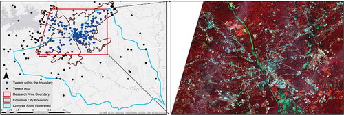
A severe flood occurred in 2015 in South Carolina due to consecutively intense precipitation on October 1st – 5th from Hurricane Joaquin. This study selects the City of Columbia as our study area (Figure 1). It is located in Richland and Lexington Counties in the central part of South Carolina. Congaree River, joined by Saluda River and Broad River in the north, is the largest flowing water bodies in its metropolitan area. The 2015 Flood in Columbia reached a 1000-year event level, whereas other areas of the state reached a 500-year level (Feaster, Shelton, and Robbins 2015; Musser et al. 2016). As shown in Figure 1, the study area covers majority of the city and is located in the upstream of the Congaree River Watershed. The 2015 SC Flood caused severe damage to public infrastructures, houses, and personal properties of this urban watershed (Li et al. 2018).

Figure 1. The study area in the City of Columbia and Congree River Watershed, SC. The ALI image (acquired 10/08/2015) is displayed in a standard false color.

Datasets

Satellite imagery during the peak flood event was not available in the study area due to heavy cloud covers. The earliest cloud-free image was acquired from the EO-1 Advanced Land Imager (ALI) on 8 October 2015, 3 days after the peak flood (as shown in Figure 1). It has 30-m resolution in multispectral bands. Functional haze removal in the ATCOR2 module of Erdas/Imagine was applied, and atmospheric correction was performed to convert digital numbers of the ALI image to surface reflectance.

Twitter data during the 2015 SC Flood were analysed. For each tweet posting the flood incident, its posting time and geographic location (latitude and longitude) were extracted, which renders valuable temporal and spatial information of this incident. In previous studies, our research team has generated a tweets pool containing 1,279,325 tweets with exact longitude and latitude using Twitter Stream API and REST API (Li et al. 2018). A keyword matching algorithm was then applied to further select flood-related tweets, which were manually checked to sort out those whose content (text, picture or both) matched well with their coordinates (pictures were checked through Google Earth). Among hundreds of tweets in our research area that passed the spatial restraint and keywords restraint, 18 tweets were verified to be flood related, posted in research area during the peak flooding dates of Oct. 3–4, and their contents matched well with their longitude and latitude. Their locations (Figure 2(a)) were used in this study to represent the flooded conditions at these locations.

Figure 2. Spatial distributions of verified flood-related tweets (a) and official flash flood points (b).

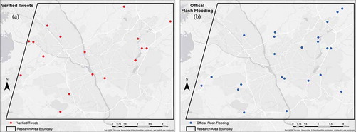
More official data about the 2015 SC Flood were released after the event. In this study, the flash flood data points, representing locations under flash flood, were downloaded from the National Weather Service (NWS) and National Oceanic and Atmospheric Administration (NOAA) (http://www.nws.noaa.gov/gis/shapepage.htm). According to the metadata, this dataset contains 23 flash flood points across the study area, all reported on Oct. 4^th when intensive rainfall happened (Figure 2(b)). Both tweets and flash flood data points were used in this study. For the convenience of description, both of them are named VGI points in the remaining sections.

Other data utilized in this study include the 3-m DEM downloaded from South Carolina Department Natural Resources (http://www.dnr.sc.gov/GIS/lidar.html). Also, the official survey-based flood inundation map, published in February 2016, was downloaded from the U.S. Geological Survey (USGS) flood inundation mapping (FIM) program (https://water.usgs.gov/osw/flood_inundation). It provides an authoritative flood extent, which serves as the reference data to evaluate our model performance.

Methodology

The method of the study is designed in four steps (Figure 3). First, with a single VGI point, an IDW-implemented Height Filter was introduced to create a probability index distribution (PID) layer, which represent a single estimation (merely based on this VGI point) of areas being flooded. After that, the NDWI was extracted from the surface reflectance of the ALI image. For each PID layer, a Gaussian-kernel distance-decay approach was developed to calculate a NDWI-curved moisture weight of this layer. A flood probability model was finally developed to produce an integrated flood probability map (FPM) of the study area. The performance of the model was evaluated by comparing the model results with the Official USGS inundation map.

VGI points: IDW-implemented probability index distributions (PIDs)

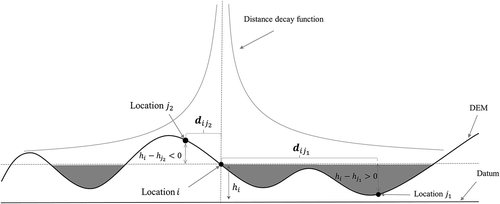
Assume we have a location that is flooded (VGI point) and location that is a random location in the same area. We believe that, as the elevation of increases, location is less likely to be flooded. In addition, the Tobler’s Law indicates that closer objects have stronger connections. In this case, the flooding probability is assumed to be negatively correlated with the distance between and , i.e., a location closer to the flooded location has a higher chance of being flooded than those further away. Based on a flooded VGI location , the differential height (DH) at location is defined as:

1)

where and represent the elevation of location and , respectively. denotes either 0 when or the potential height difference between the two points when .

Adopting the inverse distance weighting method in Li et al. (2018), given a flooded VGI location , the IDW-implemented PIDs at a random location is calculated:

(2)

where represents the Euclidean distance between location and . and are power parameters to adjust the influence of and , respectively. Both and are set to 1 for simplification (Li et al. 2018).

Figure 4 illustrates the idea of the IDW-implemented height filter for a given VGI point. The solid curve line represents the actual elevation, the horizontal dashed line is the water surface derived from Location , and the area filled with blue represents the area below location . The flood possibility within this area is weighted using the distance decay function in Equation (2). Each VGI point provides an independent, single-estimation PID layer for the whole study area.

Figure 3. Flowchart of the methodological design.

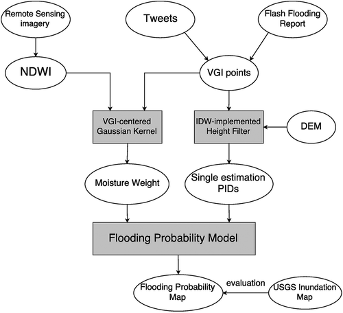
Figure 4. Illustration of variables used in Equations (1) and (2).

NDWI and VGI-centered Gaussian kernel

People who live close to a flood incident tend to post more flood-related information on social media. However, this very spatial characteristic of tweets challenges a simple yet common assumption that locations: higher flood-related tweets density suggest higher possibility of being flooded. Actually, more flood-related tweets in an area does not necessarily mean a higher flood possibility. Rather, it may simply come from a high density of Twitter users (De Albuquerque et al. 2015). To reduce the intrinsic uncertainties due to their strong correlation to population density, this study constructs the weight of VGI points from the satellite-extracted surface wetness variations, i.e. a higher weight is given to a VGI point if the satellite-extracted wetness around this area is also higher.

The NDWI is adopted to indicate ground wetness in the study area and is calculated as (Gao 1996):

(3)

where and are surface reflectance of green and SWIR bands, respectively. NDWI is positively related to land surface wetness. Cells with higher NDWI represent moister conditions. Water bodies have the highest NDWI and could be easily delineated. To facilitate future calculation and interpretation, we rescaled it to a range of [0, 2000] by multiplying the original NDWI with 1000 and adding a constant of 1000.

The ALI image was acquired on Oct. 8^th, 3 days after the peak flooding event. We assume that the image-extracted ground wetness conditions still positively reflect the real-time, VGI-posted floods within the 3-day lag. Here, a Gaussian kernel weighting algorithm was developed to aggregate the NDWI of all pixels in the kernel centered at a VGI point. The NDWI influence is gradually weaker when a pixel is further away from the VGI point. Compared with traditional inverse distance decay function, the Gaussian kernel we used results in a smoother distance decay effect. A smoother distance decay effect is less sensitive to locational discrepancy as it accounts for the wetness dynamics surrounding a VGI, thus greatly compensating the common concern of VGI’s inaccurate geolocation.

Similarly, given the location of a VGI point that was flooded, location represents a random pixel within the kernel. We assume the following statements to be true:

• Location with higher NDWI has a higher chance to be flooded, and that with lower NDWI has a lower chance;

• For location closer to the VGI point , its NDWI contributes more to the flood incident posted in this area.

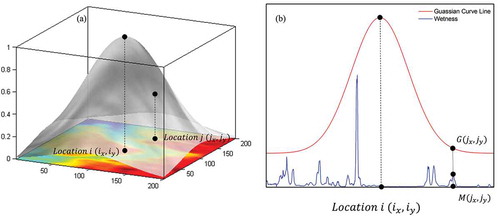
Figure 5 demonstrates the idea of overlapping the Gaussian surface to the NDWI surface. For a VGI point centered at the kernel, the moisture weight to its PID layer can be defined as:

(4)

Figure 5. A three-dimensional Gaussian surface overlapped with the NDWI surface (a) and a two-dimensional profile (b).

where location is a random pixel in the kernel, and denotes its NDWI value. denotes the value of Gaussian surface at location . In this study, we use a standardized two-dimensional Gaussian surface which satisfies:

(5)

The bandwidth, h, controls the shape of the Gaussian surface. The Gaussian function and the bandwidth are defined as follows:

(6)

T he rationale of introducing is that, by adjusting the bandwidth, we are able to manipulate the size of the interested region. A smaller bandwidth allows a steeper bell-shaped Gaussian surface function, giving more importance to pixels closer to the center. The contribution weakens dramatically as a pixel is located further away. A larger bandwidth, on the contrary, allows a larger kernel size and a smoother weighting surface.

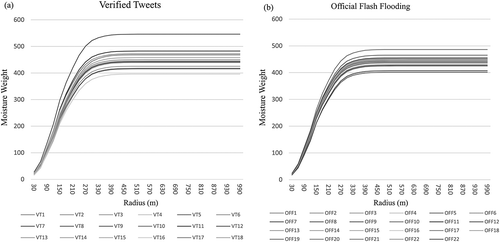
We performed a sensitivity analysis to identify an optimal h value. When assigning a value, we gradually increased the radius of R for each VGI point from 1 pixel (30 m) to 33 pixels (990 m) in an interval of 30 m. Figure 6 demonstrates the sensitivity of NDWI weight on the increase of radius R at = 15,000 m. The weight gradually reaches the saturation point when R reaches to around 360 m for both the verified tweets (Figure 6(a)) and flash flood points (Figure 6(b)), indicating that the NDWIs of the area within a 360-m distance are heavily weighted. We assume that a 360-m buffer fairly represents the wetness dynamics around a VGI point. Therefore, we decided to set bandwidth as 15,000 m in this study, with which a 360-m radius around a certain VGI contributes more to the total moisture weight of this point.

Figure 6. Sensitivity analysis of for NDWI weights at the verified tweets (a) and the NOAA flash flood points (b).

The RS/VGI integrated flood probability model

Using the two weighting components (PID and Gaussian kernel) described above, a final FPM is generated by integrating the moisture weight to each PID layer. The moisture weights for all VGI points have been standardized to a range from 0 to 1. It should be noted that all VGI points are treated equally in terms of their confidence level. In other words, no extra weights were assigned based on their authoritativeness. The FPM at any location in the study area is defined as follows:

(7)

The proposed model is implemented in Python environment, which renders a coding platform for automatically chaining different modules described above. At each pixel of the study area, the model generates a FPM indicating the probability of being flooded at this location.

Results and discussion

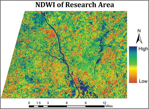
Figure 7 demonstrates the NDWI distributions of the study area. In general, the NDWI along the Congaree River remains high and the flood remnants still cover a broad swath of agricultural lands and wetlands in the southeast of the city and forests in the north.

Figure 7. The NDWI distribution of the study area.

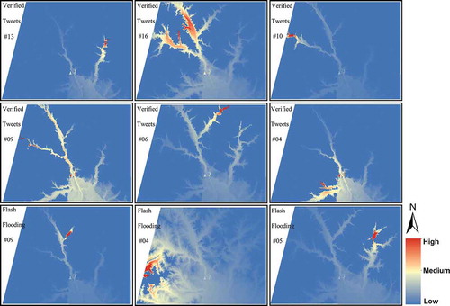
Based on the IDW rule and elevation variations, a continuous PID layer was extracted using each VGI point. A total of 41 PID layers were extracted from 18 tweets and 23 NOAA flash flood points. Figure 8 demonstrates several examples of the single-estimation PID layers. Darker blue area in the figure indicates lower flood probability, whereas red area indicates higher probability. Figure 8 shows that the contribution of the center VGI decreases as a location is moving further away from this VGI (according to the IDW rule, influence of each VGI is inversely proportional to the distance).

Figure 8. Examples of flood probability map based on single VGI point.

Within a Gaussian kernel, a moisture weight was assigned to each single-estimation PID. A final FPM was calculated by summing the moisture-weighted PIDs, and was standardized in a range of [0, 1] (Figure 9(a)). It shows a continuous surface of probability ranking across the study area, and therefore, provides the flood severity dynamics that could be used for a more quantitative assessment of the flood.

Figure 9. The final flood probability map (FPM) (a) and the FPM overlaid with USGS inundation map (grey shaded) and its map boundary (black line) (b).

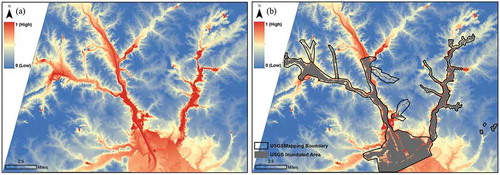
The resulted FPM map was evaluated with the USGS official inundation map. In Figure 9(b), the USGS survey boundary (black outline) is overlaid to the FPM. The grey zone within the boundary represents the USGS-surveyed flooded area. It should be noted that USGS only examined areas within the boundary. Areas falling outside boundary were not surveyed. In general, our FPM areas with high flood probability matched well with the USGS inundation map within its boundary. Beyond the USGS survey boundary, the FPM map provided continuous probabilities for the entire study area. In addition, instead of sending people to the flooded area for real-time ground survey, the only labor involved in our proposed approach was the verification of VGI points. Compared to the massive ground survey process, our proposed FPM approach is much less time- and labor-consuming.

The binary USGS inundation map within its survey boundary is the only official source of flood extents in this study, which limits the quantification of the validity of our proposed model. However, by visually and statistically comparing the histogram patterns, some comparative conclusions still can be drawn.

Firstly, a histogram comparison between the FPM map and the USGS inundation map was performed. Figure 10(a) illustrates the FPM histogram for the whole study area (cells with FPM = 0 were not considered). In general, there was a decreasing trend for cell numbers when the index increased. The mean FPM value for the whole study area was 0.131. After we constrained the model output within the USGS inundation boundary, the results indicated a normal distribution with a mean value of 0.496 (Figure 10(b)). This indicates that the areas with high probabilities generated from our model are highly correlated with the flooded area in the USGS inundation map. Figure 10(c) shows that our model successfully captures the USGS inundated areas. Areas with higher flooding probability index are more likely to be included within the USGS inundation boundary as the two lines in Figure 10(c) continue to approach each other. An abrupt increase occurs when flood probability reaches the value of 1, possibly explained by the discontinuous characteristic of the IDW distance decaying function.

Figure 10. The FPM histogram for the entire study area (a); the FPM histogram within the USGS inundation boundary (b); the FPM histograms for the entire study area and that within the USGS inundation boundary (c).

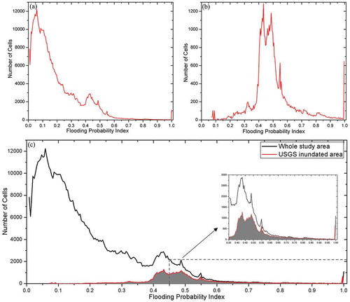
We further summarized the FPM values within the USGS-extracted inundation area. Overall, 72.04% of the inundation area had high FPM values of 0.4–0.6 and 10.11% in 0.6–0.8. These indicate that our results match well with the official inundation map.

Unlike traditional hydrological modeling, our method requires much less landscape-based inputs, thus making it easy to be generalized and applied for other flooding cases. Moreover, this new weighting method separates the confidence level of VGI from its intrinsic relation to population, providing a more scientific and robust weighting approach based on the moisture measurement (NDWI) obtained from remote sensing imagery. In addition, by viewing remote sensing as a weight giving source instead of a major mapping source, we largely reduced the intrinsic flaws in temporal resolution of remote sensing data.

Modified from the geostatistical model in Li et al. (2018), our proposed method combines the spatially clustered VGI points with continuous observation from satellite imagery. It considers three different weights including distance, relative elevation, and NDWI. Unlike the traditional point interpolation methods, the proposed method captures not only the variance of geolocation and elevation, but also the spatially continuous variance of moisture status from the image. Theoretically, more attention should be given to a certain area if it remains wetter after the flood event. The ground moisture (NDWI) distribution in a kernel centered at each VGI point attaches the moisture condition to those VGI points, providing a more comprehensive assessment of the flood probability from each VGI point. Therefore, this weighting approach yields a more objective estimation than the Li model (Li et al. 2018) that heavily relies on the tweets density.

The proposed method is able to produce a near-real time flood estimation once a satellite image is acquired. It takes much shorter time than traditional surveying approach. Flood-related tweets and official flash flood reports can be acquired in real time and a post-event image can be acquired within several days. Once all the required inputs are ready, with our current processing approach, the running time of the proposed model on a single computer is around 9 min.

One limitation of this method, however, is the time lag of post-event remote sensing imagery. In this study, a three-day lag ALI image was used to generate the NDWI under the assumption that soil moisture status fairly reflects the flood incidents 3 days ago. As the time lag becomes larger, their correlation would certainly go down until null. An image with a short time lag is highly recommended to be included in the model. Another limitation is the uncertainties when using the open source VGI data. The extraction of flood-related tweets from tweets pool based on current text matching technique often fails to guarantee the validity of text-based tweets. Further manual verification after keyword matching is still needed to assure the relevance and improve the accuracy. Another issue needed to be concerned is the sample size of VGI points used in this study. Limited by the uncertainty raised by the traditional text matching algorithm, the semi-automatic workflow of selecting tweets we used in this study requires labor involved checking. This process demands that the tweets content (text, photos, or both) have a strong correlation with their exact location, which largely reduce the number of available tweets to be used in the study. However, a small amount of verified flood-related tweets with strong connect to their intrinsic geolocation is preferred than a large amount of less related tweets generated through a full automatic process. We believe that with the rapid development of social media and machine learning technology, this process could be automated eventually with an improving accuracy.

Conclusion

Rapid extraction of flood inundation has always been critical for emergency managers and local authorities to conduct quick assessment of flood damage and provide support in areas with immediate attention. Taking the 2015 South Carolina Flood as an example, this study develops a near-real time flood probability map to improve situational awareness during a flooding event. We developed a rapid flood-mapping model by firstly, generating PID layers through the integration of verified VGI points (verified flood-related tweets and flash flood locations issued by local government) and DEM, and secondly, attaching weights to them via image-extracted land surface wetness conditions. Superior to traditional surveying approaches, the proposed model is able to provide a continuous flood probability ranking in a much shorter time throughout the study area. With the spatially continuous inputs of surface wetness, it also reduces the uncertainties raising from the validity of tweets points in geostatistical studies that merely rely on social media by separating the confidence level of tweets from its intrinsic relation to population density, thus providing a more robust weighting scheme based on wetness measurements. In addition, the proposed model is compatible with other crowdsourcing and authoritative databases, allowing other supplemental information to be added in the future.

We believe that the methodology used in this article could seed a wide range of future flood studies for rapid and improved flood situational awareness in a city as well as at a regional level. The resulted flood probability map improves situational awareness right after a flood event by connecting VGI with surface wetness conditions, aiding local authorities and responders with better decision-making and responses.

Disclosure statement

No potential conflict of interest was reported by the author.

References

- Adhikari, P., Y. Hong, K. R. Douglas, D. B. Kirschbaum, J. Gourley, R. Adler, and G. R. Brakenridge. 2010. “A Digitized Global Flood Inventory (1998–2008): Compilation and Preliminary Results.” Natural Hazards 55 (2): 405–422. doi:10.1007/s11069-010-9537-2.
- Ashley, S. T., and W. S. Ashley. 2008. “Flood Fatalities in the United States.” Journal of Applied Meteorology and Climatology 47 (3): 805–818. doi:10.1175/2007JAMC1611.1.
- Blöschl, G., and M. Sivapalan. 1995. “Scale Issues in Hydrological Modelling: A Review.” Hydrological Processes 9 (3–4): 251–290. doi:10.1002/(ISSN)1099-1085.
- Chen, J., A. A. Hill, and L. D. Urbano. 2009. “A GIS-based Model for Urban Flood Inundation.” Journal of Hydrology 373 (1–2): 184–192. doi:10.1016/j.jhydrol.2009.04.021.
- Davranche, A., B. Poulin, and G. Lefebvre. 2013. “Mapping Flooding Regimes in Camargue Wetlands Using Seasonal Multispectral Data.” Remote Sensing of Environment 138: 165–171. doi:10.1016/j.rse.2013.07.015.
- de Albuquerque, J. P., B. Herfort, A. Brenning, and A. Zipf. 2015. “A Geographic Approach for Combining Social Media and Authoritative Data Towards Identifying Useful Information for Disaster Management.” International Journal of Geographical Information Science 29 (4): 667–689. doi:10.1080/13658816.2014.996567.
- Di Baldassarre, G., G. Schumann, P. D. Bates, J. E. Freer, and K. J. Beven. 2010. “Flood-Plain Mapping: A Critical Discussion of Deterministic and Probabilistic Approaches.” Hydrological Sciences Journal–Journal des Sciences Hydrologiques 55 (3): 364–376. doi:10.1080/02626661003683389.
- Douben, K.-J. 2006. “Characteristics of River Floods and Flooding: A Global Overview, 1985–2003.” Irrigation and Drainage 55 (S1): S9–21. doi:10.1002/(ISSN)1531-0361.
- Efstratiadis, A., and D. Koutsoyiannis. 2010. “One Decade of Multi-Objective Calibration Approaches in Hydrological Modelling: A Review.” Hydrological Sciences Journal–Journal Des Sciences Hydrologiques 55 (1): 58–78. doi:10.1080/02626660903526292.
- Feaster, T. D., J. M. Shelton, and J. C. Robbins. 2015. Preliminary Peak Stage and Streamflow Data at Selected USGS Streamgaging Stations for the South Carolina Flood of October 2015 (ver. 1.1, November 2015). U.S. Geological Survey Open-File Report 2015–1201, 19 p. doi:10.3133/ofr20151201.
- Gao, B.-C. 1996. “NDWI—A Normalized Difference Water Index for Remote Sensing of Vegetation Liquid Water from Space.” Remote Sensing of Environment 58 (3): 257–266. doi:10.1016/S0034-4257(96)00067-3.
- Goodchild, M. F. 2007. “Citizens as Sensors: The World of Volunteered Geography.” GeoJournal 69 (4): 211–221. doi:10.1007/s10708-007-9111-y.
- Herfort, B., J. P. De Albuquerque, S. J. Schelhorn, and A. Zipf. 2014. “Exploring the Geographical Relations between Social Media and Flood Phenomena to Improve Situational Awareness.” In Connecting a Digital Europe through Location and Place, 55–71. Cham: Springer.
- Herfort, B., M. Eckle, J. P., de Albuquerque, & A. Zipf. 2015. “Towards Assessing the Quality of Volunteered Geographic Information from OpenStreetMap for Identifying Critical Infrastructures. ISCRAM, May.
- Ho, L. T. K., M. Umitsu, and Y. Yamaguchi. 2010. “Flood Hazard Mapping by Satellite Images and SRTM DEM in the Vu Gia–Thu Bon Alluvial Plain, Central Vietnam.” International Archives of the Photogrammetry, Remote Sensing and Spatial Information Science 38 (Part 8): 275–280.
- Horita, F. E., J. P. De Albuquerque, L. C. Degrossi, E. M. Mendiondo, and J. Ueyama. 2015. “Development of a Spatial Decision Support System for Flood Risk Management in Brazil that Combines Volunteered Geographic Information with Wireless Sensor Networks.” Computers & Geosciences 80: 84–94. doi:10.1016/j.cageo.2015.04.001.
- Horita, F. E. A., L. C. Degrossi, L. F. G. De Assis, A. Zipf, and J. P. De Albuquerque. 2013. “The Use of Volunteered Geographic Information (VGI) and Crowdsourcing in Disaster Management: A Systematic Literature Review.” Proceedings of the Nineteenth Americas Conference on Information Systems, Chicago, IL, August 15–17.
- Jain, S. K., R. D. Singh, M. K. Jain, and A. K. Lohani. 2005. “Delineation of Flood-Prone Areas Using Remote Sensing Techniques.” Water Resources Management 19 (4): 333–347. doi:10.1007/s11269-005-3281-5.
- Kulkarni, A. T., J. Mohanty, T. I. Eldho, E. P. Rao, and B. K. Mohan. 2014. “A Web GIS Based Integrated Flood Assessment Modeling Tool for Coastal Urban Watersheds.” Computers & Geosciences 64: 7–14. doi:10.1016/j.cageo.2013.11.002.
- Li, Z., C. Wang, C. T. Emrich, and D. Guo. 2018. “A Novel Approach to Leveraging Social Media for Rapid Flood Mapping: A Case Study of the 2015 South Carolina Floods.” Cartography and Geographic Information Science 45 (2): 97–110.
- Mallinis, G., I. Z. Gitas, V. Giannakopoulos, F. Maris, and M. Tsakiri-Strati. 2013. “An Object-Based Approach for Flood Area Delineation in a Transboundary Area Using ENVISAT ASAR and LANDSAT TM Data.” International Journal of Digital Earth 6 (sup2): 124–136.
- McFeeters, S. K. 1996. “The Use of the Normalized Difference Water Index (NDWI) in the Delineation of Open Water Features.” International Journal of Remote Sensing 17 (7): 1425–1432. doi:10.1080/01431169608948714.
- Messner, F., and V. Meyer. 2006. “Flood Damage, Vulnerability and Risk Perception–Challenges for Flood Damage Research.” In Flood Risk Management: Hazards, Vulnerability and Mitigation Measures, 149–167. Dordrecht: Springer.
- Musser, J. W., K. M. Watson, J. A. Painter, and A. J. Gotvald. 2016. Flood-Inundation Maps of Selected Area Affected by the Flood of October 2015 in Central and Coastal South Carolina (No. 2016-1019). US Geological Survey.
- Njoku, E. G., and D. Entekhabi. 1996. “Passive Microwave Remote Sensing of Soil Moisture.” Journal of Hydrology 184 (1–2): 101–129. doi:10.1016/0022-1694(95)02970-2.
- Palacios-Orueta, A., S. Khanna, J. Litago, M. L. Whiting, and S. L. Ustin. 2006. “Assessment of NDVI and NDWI Spectral Indices Using MODIS Time Series Analysis and Development of a New Spectral Index Based on MODIS Shortwave Infrared Bands.” Proceedings of the 1st International Conference of Remote Sensing and Geoinformation Processing, 207–209, Trier. http://ubt,opus.hbz-nrw,de/volltexte/2006/362/pdf/03-rgldd-session2,pdf.
- Palen, L., K. Starbird, S. Vieweg, and A. Hughes. 2010. “Twitter-Based Information Distribution during the 2009 Red River Valley Flood Threat.” Bulletin of the American Society for Information Science and Technology 36 (5): 13–17. doi:10.1002/(ISSN)1550-8366.
- Poser, K., and D. Dransch. 2010. “Volunteered Geographic Information for Disaster Management with Application to Rapid Flood Damage Estimation.” Geomatica 64 (1): 89–98.
- Qiao, C., J. Luo, Y. Sheng, Z. Shen, Z. Zhu, and D. Ming. 2012. “An Adaptive Water Extraction Method from Remote Sensing Image Based on NDWI.” Journal of the Indian Society of Remote Sensing 40 (3): 421–433. doi:10.1007/s12524-011-0162-7.
- Rasid, H., W. Haider, and L. Hunt. 2000. “Post-Flood Assessment of Emergency Evacuation Policies in the Red River Basin, Southern Manitoba.” Canadian Geographer 44 (4): 369–386. doi:10.1111/cag.2000.44.issue-4.
- Renard, B., D. Kavetski, G. Kuczera, M. Thyer, and S. W. Franks. 2010. “Understanding Predictive Uncertainty in Hydrologic Modeling: The Challenge of Identifying Input and Structural Errors.” Water Resources Research 46 (5). doi:10.1029/2009WR008328.
- Schnebele, E., G. Cervone, S. Kumar, and N. Waters. 2014. “Real Time Estimation of the Calgary Floods Using Limited Remote Sensing Data.” Water 6 (12): 381–398. doi:10.3390/w6020381.
- Schnebele, E., and N. Waters. 2014. “Road Assessment after Flood Events Using Non-Authoritative Data.” Natural Hazards and Earth System Sciences 14 (4): 1007–1015. doi:10.5194/nhess-14-1007-2014.
- Stefanidis, S., and D. Stathis. 2013. “Assessment of Flood Hazard Based on Natural and Anthropogenic Factors Using Analytic Hierarchy Process (AHP).” Natural Hazards 68 (2): 569–585. doi:10.1007/s11069-013-0639-5.
- Townsend, P. A., and S. J. Walsh. 1998. “Modeling Floodplain Inundation Using an Integrated GIS with Radar and Optical Remote Sensing.” Geomorphology 21 (3–4): 295–312. doi:10.1016/S0169-555X(97)00069-X.
- Tralli, D. M., R. G. Blom, V. Zlotnicki, A. Donnellan, and D. L. Evans. 2005. “Satellite Remote Sensing of Earthquake, Volcano, Flood, Landslide and Coastal Inundation Hazards.” ISPRS Journal of Photogrammetry and Remote Sensing 59 (4): 185–198. doi:10.1016/j.isprsjprs.2005.02.002.
- Triglav-Čekada, M., and D. Radovan. 2013. “Using Volunteered Geographical Information to Map the November 2012 Floods in Slovenia.” Natural Hazards and Earth System Sciences 13 (11): 2753–2762. doi:10.5194/nhess-13-2753-2013.
- Van der Sande, C. J., S. M. De Jong, and A. P. J. De Roo. 2003. “A Segmentation and Classification Approach of IKONOS-2 Imagery for Land Cover Mapping to Assist Flood Risk and Flood Damage Assessment.” International Journal of Applied Earth Observation and Geoinformation 4 (3): 217–229. doi:10.1016/S0303-2434(03)00003-5.
- Villarini, G., J. A. Smith, M. L. Baeck, P. Sturdevant-Rees, and W. F. Krajewski. 2010. “Radar Analyses of Extreme Rainfall and Flooding in Urban Drainage Basins.” Journal of Hydrology 381 (3–4): 266–286. doi:10.1016/j.jhydrol.2009.11.048.
- Yin, J., M. Ye, Z. Yin, and S. Xu. 2015. “A Review of Advances in Urban Flood Risk Analysis over China.” Stochastic Environmental Research and Risk Assessment 29 (3): 1063–1070. doi:10.1007/s00477-014-0939-7.