Spatial prediction based on Third Law of Geography

ABSTRACT

Current methods of spatial prediction are based on either the First Law of Geography or the statistical principle or the combination of these two. The Second Law of Geography contributes to the revision of these methods so they are adaptive to local conditions but at the cost of increasing demand for samples. This paper presents a new thinking about spatial prediction based on the Third Law of Geography which focuses on the similarity of geographic configuration of locations. Under the Third Law of Geography, spatial prediction can be made on the basis of the similarity of geographic configurations between a sample and a prediction point. This allows the representativeness of a single sample to be used in prediction. A case study in predicting spatial variation of soil organic matter content was used to compare the spatial prediction based the Third Law of Geography with those based on the First Law and the statistical principle. It is concluded that spatial prediction based on the Third Law of Geography does not require samples to be over certain size nor to be of a particular spatial distribution to achieve a high quality prediction. The prediction uncertainty associated with spatial prediction based on the Third Law of Geography is more indicative to quality of the prediction, thus more effective in allocating error reduction efforts. These properties make spatial prediction based on the Third Law of Geography more suitable for prediction over large and complex geographic areas.

KEYWORDS:

• First Law of Geography
• Second Law of Geography
• Third Law of Geography
• spatial prediction
• spatial interpolation
• Kriging
• soil mapping
• geographic configuration

1. Introduction

Information on the spatial variation (spatial data) of geographic variables (phenomena) (such as vegetation, soils, habitat suitability, and hazard susceptibility) is essential for geographic modelling and management decision making at local, regional, and global scales (Goodchild, Parks, and Steyaert 1993; Goodchild, Steyeart, and Parks 1996; Miller and White 1998; Van Westen, Castellanos, and Kuriakose 2008). Obtaining spatial data is a key research area in geography, particularly in the field of geographic information science (Tomlinson, Calkins, and Marble 1976; Goodchild 2004a; Cruden 2017). Spatial prediction (sometimes also referred to as spatial interpolation, predictive mapping) is one of the major approaches for achieving that, particularly for variables, such as soil conditions, habitat suitability, hazards susceptibility, for which other methods such as remote sensing are ineffective in obtaining satisfactory results (Skidmore 2003).

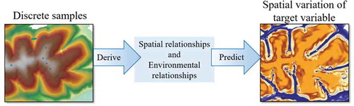
The basic idea of spatial prediction is to use what we have already known at locations to estimate the values of a geographic variable (referred to as the target variable) which are unknown at these locations or other locations (referred to as prediction points). Spatial prediction is typically done in the process as shown in Figure 1. First, a set of discrete samples are collected over the area of interest. Second, information collected at these samples are then analyzed to derive relationships describing how the values of the target variable is related to the information collected at these samples. Finally, these relationships are used to predict the values of the target variable at prediction points. The key to the success and applicability of spatial prediction are the underlying assumptions employed in describing the relationships and the way in which how these relationships are characterized.

Figure 1. Derivation of relationships from samples for spatial prediction.

This paper first examines how the basic principles, specifically the First and Second Laws of Geography as referred to by some scholars (Tobler 1970; Goodchild 2004b) and the statistic principle, are used to provide the underlying assumptions for describing and characterizing the relationships used in spatial prediction and the limitations in applying these principles to spatial prediction. The paper will then present another widely known and commonly used principle of geography, one may refer to it as the Third law of Geography, under the context of addressing issues faced with the other principles in spatial prediction. The utility of Third Law of Geography is illustrated through the development and application of a completely new approach in spatial prediction for soil mapping.

2. Existing principles in spatial prediction and their limitations

The key issues in spatial prediction are the underlying assumptions used to describe the relationships and the way how the relationships are characterized. There are three basic principles, namely the First Law of Geography, statistical principle and the Second Law of Geography, used in spatial predictions as described below.

2.1. The First Law of Geography for spatial prediction

The first principle used in spatial prediction is that attribute values of a target variable are spatially related (spatial autocorrelation) and that locations which are closer would have more similarity values of attributes than locations are further apart. Danie Krige is among the first to use this principle for spatial prediction in his effort to plot the gold grades over space (Krige 1951). Matheron (1963) later developed the theoretical basis for the method which led to a much celebrated family of methods, now referred to as the Kriging methods. Other spatial prediction techniques based on this principle include nearest neighbours, moving average (local sample mean), and inverse distance weighted (IDW) (Isaaks and Srivastava 1989; Goovaerts 1999). Tobler, in his 1970 paper, stated this important geographic principle as the First Law of Geography through his famous statement ‘Everything is related to everything else, but near things are more related than distant things’ (Tobler 1970).

The First Law of Geography states an important property of geographic variation (spatial variation). The key issue in using this important property for spatial prediction is to design a mean to capture and represent this property of spatial variation. We use the ordinary Kriging method as an example to illustrate how this important property is represented and used in spatial prediction as well as the requirements associated with such use of this principle (Figure 2).

Figure 2. An illustration of the use of the First Law of Geography in ordinary Kriging and the limitations of such use. Samples are used to define how the semivariance changes with respect to distance between pair of points to create a semivariogram, to which a semivariogram model is fitted. The semivariogram model is then used to compute the semivariances (${\tilde{\gamma }}_{ij}$ and ${\tilde{\gamma }}_{i0}$) needed in the process of minimizing the objective function to determine the weights which will be assigned to the sample points nearby to compute the attribute value (${\hat{Z}}_0$) at prediction point 0.

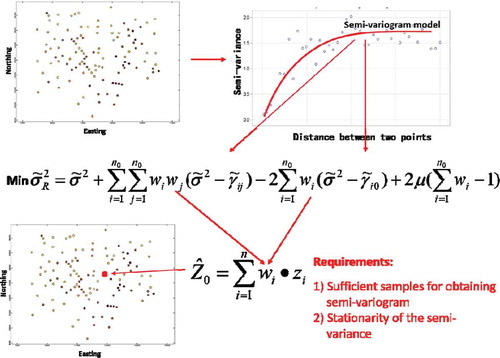
Like any other spatial prediction techniques which are based on the First of Geography, the key issue the Kriging method needs to solve is how to allocate the weights to nearby samples for estimating the value of the target variable at a prediction point. The Kriging method determines the weight allocation by minimizing the error variance model as shown in Equation 1.

(1) $\begin{array}{rl}& {\tilde{\sigma }}_R^2={\tilde{\sigma }}^2+\sum _{i=1}^{n_0}\sum _{j=1}^{n_0}{w}_i{w}_j({\tilde{\sigma }}^2-{\tilde{\gamma }}_{ij})\\ & -2\sum _{i=1}^{n_0}{w}_i({\tilde{\sigma }}^2-{\tilde{\gamma }}_{i0})\\ & +2\mu (\sum _{i=1}^{n_0}{w}_i-1)\end{array}$(1)

Where

${\tilde{\sigma }}_R^2$ is the error variance for the prediction point and is to be minimized, ${\tilde{\sigma }}^2$ is the sill of the semivariogram, w_i and w_j are the weights assigned to sample i and sample j, n₀ is the number of samples involved for predicting the value at prediction point 0, μ is the Lagrange parameter (dummy variable), ${\tilde{\gamma }}_{ij}$ is the semivariance for the distance between sample i and sample j which is computed from the semivariogram model given the distance between sample i and sample j. Similarly, ${\tilde{\gamma }}_{i0}$ is the semivariance for the distance between sample i and the prediction point 0. Once determined, the weights will be used in a weighted average function (Equation 2) together with the attribute values at the sample points involved to estimate attribute value at the prediction point 0.

(2) ${\hat{Z}}_0=\sum _{i=1}^{n_0}{w}_i\bullet z_i$(2)

Where

${\hat{Z}}_0$ is the attribute value to be predicted at the prediction point 0, Z_i is the attribute value at sample point i, w_i is the weight assigned to sample point i (summed up to 1), n₀ is the total number of samples involved in the prediction of the attribute value at prediction point 0.

Clearly, the predicted value is dependent on the weight (w_i) assigned to each sample point involved given that Z_i and n₀ are fixed. If the weight assigned to a sample represents the spatial relationship between this sample point and the prediction point well, then the predicted value would be a good approximation of the real value at the site 0. This is conditioned on the fact that the computed semivariances between sample points (${\tilde{\gamma }}_{ij}$) and that between a sample and the prediction point (${\tilde{\gamma }}_{i0}$) from the semivariogram model are good representations of the actual differences in attribute values between these points. This in turn depends on how well the semivariogram model represents the spatial autocorrelation that exists in the study area. If it does not, then the computed semivariances are not a good representation of the reality, and in turn the weights assigned to the sample points cannot capture the relationships between the prediction point and the sample points. Certainly, the predicted value will not be a good approximation of the reality at the prediction point.

From what has been presented above, we can conclude that in order for the Kriging method to work the semivariogram model must meet the requirement referred to as the stationarity assumption in addition to the need of sufficient samples to derive it. This assumption states that the semivariance (or the difference in attribute) between a pair of points only depends on distance between the two points, and it does not change with the orientation of the two points given the distance separating them is fixed, and does not change with the locations of the two points as long as their distance does not change. It is fair to say that the Kriging method requires two conditions: sufficient samples to derive the semivariogram model to describe the spatial autocorrelation of the area and the stationarity of the semivariogram model (which can be stated plainly that the spatial autocorrelation does not change over space). To some extent these two requirements are also needed for other spatial prediction techniques based on the First of Law of Geography (such as IDW).

2.2. The statistical principle for spatial prediction

Another principle used in spatial prediction is the statistical principle. Here, we use this term to refer to the statistic correlation between variables as expressed through regression analysis and to distinguish this from the geostatistical methods (such as Kriging described above). The principle assumes that there is a relationship between the value of the target variable (dependent variable) and the values from other variables (independent variables), and this relationship can be used to predict the value of the target variable at a prediction point. In this paper, we refer to the independent variables as environmental covariates (or simply covariates) and the relationship between the target variables and the covariates as covariate relationships. With the rapid development of remote sensing and geographic information processing techniques, vast amount of data on our physical and social environment have been collected and accumulated (Eldawy and Mokbel 2015). This increasing availability of data made this statistical principle not only possible but also viable to be deployed in spatial prediction. The recent development and the availability of machine learning techniques (such as decision trees, random forests, neural networks) have attracted further attention to spatial prediction based on this principle (Kanevski, Timonin, and Pozdnukhov 2009; Li et al. 2011; Ließ, Glaser, and Huwe 2012).

The key issue in using the statistical principle in spatial prediction is how to characterize the relationship between the target variable and its covariates. The techniques based on this principle are in common as to how they extract the relationships and how they apply the extracted relationship to prediction. For simplicity, we use the linear regression method as an example to illustrate how the statistical principle is used in spatial prediction as well as the requirements associated with such use of this principle (Figure 3).

Figure 3. Illustration of the statistical principle used in spatial prediction and its requirements. Samples are used to extract the relationship (f) between the target variable and a set of environmental covariates (x). The relationship is then applied together with the values of the covariates at each location to predict the value of the target variable at this location.

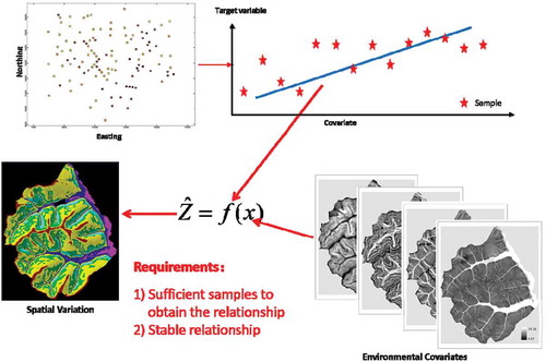
As one can see, the predicted value is dependent on f given that the values from a set of covariates are fixed. As in the spatial prediction based on the First Law of Geography, the requirements for spatial prediction based on the statistical principle are similar: 1) sufficient samples to extract the relationships and 2) the extracted relationship to be stable over the entire study area (which is similar to the stationarity assumption of the Kriging method).

2.3. The Second Law of Geography for spatial prediction

Obviously, the stationarity assumption of spatial autocorrelation and the static requirement of the extracted covariate relationship, collectively referred to as the stationarity assumption, often cannot be met because of the nature of geographic phenomena. It is difficult to imagine that these relationships (spatial or covariate) will hold static or stay the same over space considering the geographic phenomena are inherently heterogeneous. This is particularly true for large and complex geographic areas. Spatial heterogeneity of geographic phenomena has been one of the major subjects of geographic studies (Hartshorne 1939; Hartshorne 1959; Harvey 1996; Fotheringham and Brunsdon 1999; Phillips 2003; Anselin 2013). This heterogeneous nature of geographic phenomena has recently been referred to as the Second Law of Geography by Goodchild (2004b).

In recognition of what captured by the Second Law of Geography, techniques for spatial prediction have been substantially revised to account for spatial heterogeneity and to make them adaptive to local conditions. The various revisions made were to limit the spatial extent over which the extracted relationship is applied. For example, the Kriging method discussed above has been extended to many versions to account for various aspects of spatial heterogeneity. Kriging with locally varying sills was developed to adjust the extracted spatial autocorrelation to fit different areas in hope to meet the stationarity assumption (Isaaks and Srivastava 1989). Kriging within classes was designed to limit the application to the same class of geographic feature over the area so that spatial heterogeneity can be minimized (Cressie 1991). The Box-Cox Kriging was developed to constrain the spatial extent over which the extracted spatial autocorrelation is applied (Kitanidis and Shen 1996). Directional Kriging was developed to account for variation in spatial autocorrelation in different directions (Wingle and Poeter 1998). On the spatial prediction based on covariate relationship, geographic weighted regression, which has received much attention lately, forces the regression to be built and applied over local areas specified by a bandwidth (Brunsdon, Fotheringham, and Charlton 1996; Fotheringham, Brunsdon, and Charlton 2002).

2.4. The challenges of the existing spatial prediction techniques

From the above discussion we can summarize that the spatial prediction techniques based on the First Law of Geography or the statistical principle have two key requirements: sufficient samples for effectively characterizing the relationship and the stationarity of the extracted relationship over the entire study area. The techniques based on the combination of these two principles, such as co-Kriging (Stein and Corsten 1991), regression-Kriging and its variants (Odeh, McBratney, and Chittleborough 1995; Hengl, Heuvelink, and Stein 2004), have the same requirements. Although what captured in the Second Law of Geography made the corresponding spatial prediction techniques be localized to avoid the violation of the stationarity assumption, this localization does not remove the stationarity assumption from those techniques, actually demands much more samples so that the local versions of relationships (spatial or covariate) can be derived. It is fair to say that the following requirements are associated with the current principles and their uses in spatial prediction: 1) large sample set; 2) stationarity assumption; 3) small geographic areas.

These requirements or limitations might not present a serious problem if spatial prediction is only applied to generate spatial variation of geographic variables over some limited areal coverage and that there are substantial number of samples available for the area of interest and the relationships are reasonably stable over that area. It clearly would be a problem for spatial prediction to be applied over large areas with complex geographic processes, which are more than often with the increase of geographic area. This is because on one hand applying the spatial prediction techniques without these modifications to accommodate what captured by the Second Law of Geography would certainly violate the stationarity assumption of these techniques. On the other hand, it is prohibitively expensive to collect samples at the level of density and at the spatial distribution needed for the spatial prediction techniques revised under the Second Law of Geography. One might suggest that the recent increase of data collected through citizen science (Sui, Elwood, and Goodchild 2012) or volunteered geographic information (Goodchild 2007; Goodchild and Glennon 2010; Haklay 2013) would provide a viable sources of samples needed. However, samples from these sources are often ad-hoc in nature (Zhu et al. 2015a) and often do not meet the requirements imposed on the samples by these techniques. Unfortunately, when the samples do not conform to the requirements, these techniques have little ability to report the uncertainty in the results due to the failure to meet the sample requirement.

The key issue in leading to the failure in spatial prediction over large area is that the existing principles and their application in spatial prediction is to extract an ‘average’ relationship from a collection of samples and apply this ‘average’ relationship to the entire area (small or large). For example, in the Kriging method the semivariogram model describes the ‘average’ condition of spatial autocorrelation in the sample set. By ‘average’ we first mean that the semivariance computed for each lag is an average of the squared differences in attribute for pair of points separated at this distance as shown in Equation 3.

(3) $\gamma (h)=\frac{1}{2N(h)}\sum _{(i,j)|d_{ij}=h}^{N(h)}(z_j-z_i{)}^2$(3)

Where

h is the distance between two points (a pair of points), referred to as lag, γ(h) is the semi-variance in attribute for pairs with h distance apart, N(h) is the number of pairs of points with h distance apart. Z_i is the attribute value at point i, and (i,j)|d_ij = h denotes all the pairs of points which are separated by h distance. Clearly, γ(h) is an average value of the semivariance for pairs of points separated by h distance. This means that it is very possible, even more likely, that the specific semivariance between a given pair of points can be larger or smaller than this average value or can even be quite larger or smaller which makes the average value less representative.

The second aspect in our use of ‘average’ is that when the semivariogram model is fitted onto these ‘average’ semivariances at each lag, the model does not fit through these points of semivariances exactly. In all cases, the fitted model runs through the sets of points by minimizing the deviation from these points (Figure 2). This is another level of ‘averaging’. It is fair to say that the semivariances computed from the semivariogram model and used in the optimization of the error variance model (Equation 1) are the values from an average semivariogram model, which is fitted to a set of average semivariances.

Using the semivariances averaged in such ways to approximate the varying values of semivariance for pairs of points separated by h distance makes what expressed in the semivariogram model about spatial autocorrelation deviate from what existed in the sample set, which is another level of approximation of the spatial autocorrelation existed in the study area. So the spatial autocorrelation used in deriving the weight assigned to each sample point can be quite different from the spatial autocorrelation existed in the study area. For large areas or areas with high geographic complexity, this difference can be significant. The analysis on ‘averaging’ in the Kriging method can also be applied to other spatial prediction techniques based on spatial autocorrelation as well as those based on the statistical principle. This averaging not only introduces errors in the prediction but also makes these techniques unable to capture details of spatial variation properly.

Recent trends in geographic analysis have seen that the level of spatial details on spatial information has dramatically increased in addition to the increase of spatial extent of geographic analysis (Anselin 2013). This demands the spatial information to drive the analysis to be at a fine spatial resolution and over large areas. Furthermore, current geographic modelling in support of decision making demands uncertainty assessment about model results, which calls for uncertainty measures about the spatial information of the input geographic variables (Hunsaker et al. 2013; Shi 2008). Clearly, the existing spatial prediction techniques as shown through the above analysis fell short to meet these needs of emerging geographic analysis.

3. The Third Law of Geography and spatial prediction

3.1. The Third Law of Geography

In geographic analysis we more than often see studies that use similarity in geographic environment as constituted by a set of geographic variables at locations or areas to assess the similarity of other geographic variables or activities at other locations or areas. For example, in crime analysis, scholars often studied the geographic environment (configuration of geographic variables such as income, education, social amenities) over the areas where crime occurrences are high and apply the set of conditions derived to see what other areas which would be more likely to have this type of crimes (Wortley and Townsley 2016). In soil science, pedologists studied the formation of soils under certain geographic environment (the configuration of geographic variables such as climate, geology, topography, vegetation, and time) over some areas and then expected the similar soil formation processes to occur at other locations or areas with similar geographic environment (Dokuchaev 1883; Jenny 1994).

The above examples as well as other similar studies manifest another important geographic principle which has important implication for spatial prediction. We summarize this geographic principle as ‘The more similar geographic configurations of two points (areas), the more similar the values (processes) of the target variable at these two points (areas)’. One may regard this as ‘the Third Law of Geography’. The significance expressed in this statement are in the following two aspects. The first is its comparative nature. It examines the similarity of the geographic configurations of two locations and then links this similarity with the similarity of the values (the processes) of the target variable at these locations. It does not call for an explicit relationship (e.g. a mathematical model) between the geographic configuration and the value of the target variable to be established, which is significantly different from the statistical principle discussed earlier (more on this in the discussion section later).

The second aspect is the term ‘geographic configuration’ which means the makeup and the structure of geographic variables over some spatial neighbourhood around a point. It has three elements. The first element is the list of geographic variables or a set of covariates defining the geographic configuration for a given target variable. The set of geographic variables may be different for different target variables under concern. For example, if the target variable is soil organic content of top soil horizon, one may need to include climate variables (about temperature and moisture), geological variables (about parent materials), topography (redistribution of energy and matters), vegetation (about organism) and time (duration of interaction) if possible. If the target variable is crime occurrence, then the set of variables (covariates) associated with crime should be used to construct the geographic configuration. The second element in this geographic configuration is the spatial scale or the spatial granularity (the foot print or neighbourhood) over which geographic processes will manifest themselves. For example, the formation of soil requires some spatial extent for the soil formation processes to interact. Clearly, different target variables would have different spatial granularity. The third element is the hierarchy of geographic variables. In the example of soil formation, we would consider the climatic conditions to be the higher hierarchy because it controls energy and matter at much more important level than topography. Thus the evaluation of similarity in geographic configuration needs to consider these two aspects: the comparative nature and the geographic configuration.

3.2. Its implication for spatial prediction

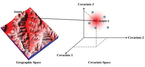
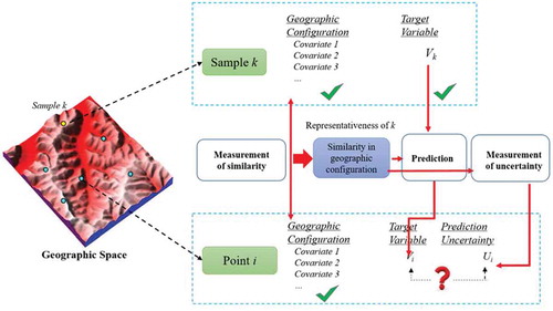
The Third Law of Geography provides a very different perspective on spatial prediction. Its comparative nature calls for prediction based on comparison of a sample point and a prediction point, rather than based on explicit relationships derived from an entire set of samples. Under this Law, we can use the representation of a single sample point, rather than the representation of an entire sample set which unavoidably is the average. The representativeness of a single sample can be expressed as shown in Figure 4. Under the notation of the Third Law of Geography, a sample point k in geographic space can be transform into the geographic configuration space as constructed by the covariates of the target variable (referred as the covariate space). The representativeness of sample k to other points can be quantified by the similarity of these points to sample k in this covariate space.

Figure 4. The representativeness of a single sample to a location of prediction can be quantified by the similarity between the geographic configurations of these two points.

The basic idea in spatial prediction using the Third Law of Geography is illustrated in Figure 5. The similarity in geographic configuration between sample point k and prediction point i is first to be computed and used as the representativeness of sample k to prediction point i. This similarity is then used as the weight in the prediction of the value of the target variable at prediction point i, together with the other involved sample points whose weights are determined similarly. This similarity together with the similarity of other sample points are also used to measure the uncertainty associated with the prediction using the samples involved. This way of spatial prediction does not require the samples to be of specific size, nor does it require the samples to be distributed in specific patterns.

Figure 5. Spatial prediction based on the Third Law of Geography. The similarity in geographic configuration between sample point k and prediction point i can be used as the representativeness of sample k to prediction point i and is used as weight in the prediction of the value of the target variable at prediction point i. This similarity is also used in measuring the uncertainty associated with the prediction.

4. Case study

We here use soil property mapping as a case study to illustrate the application of the Third Law of Geography to spatial prediction. The emphasis here is on how spatial prediction based on the Third Law of Geography differs from that based on the other principles discussed in Section 2. It is not the intent of this case study to examine the various aspects of the Third Law when applied to spatial prediction.

4.1. Study area and datasets

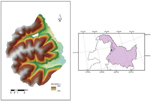
As a case of illustration, the study area is about 60 km² in size, located in Heshan farm, Nenjiang County, Heilongjiang Province of China (Figure 6). The climate condition in the study area is quite homogeneous over the study area: annual temperature ranges from −38 °C to 36 °C and the average annual precipitation is 500–600 mm. Most soils in the area were formed on deposits of silt loam loess with exception in the valley, where the parent material is fluvial deposits from up slopes. Elevation within the area ranges from 270 m to 360 m with slope gradient generally under 4°. The study area has been cultivated as cropland for over 40 years. Soybean and wheat are the main agricultural products. The soils over this area generally have a thick top-layer with naturally high organic matter content. Thus, little organic fertilizers are required to maintain a high productivity.

Figure 6. Location of study area.

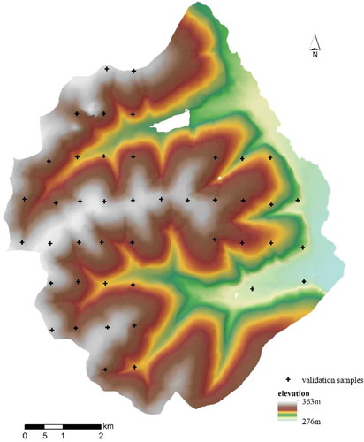
In order to see the effectiveness of spatial prediction based on the Third Law of Geography in term of low sample requirement, 10 soil samples were collected along a transect line crossing two side slopes (Figure 7). The locations of those samples were subjectively determined by soil surveyors to reveal the soil variation along a topo-sequence. Notice that the ridge areas and wide valley areas were not sampled. It is highly unlikely that those 10 soil samples can sufficiently represent the soil–environment relationships as well as the spatial autocorrelation of soil attributes in the entire study area. This provides an excellent example to illustrate the flexibility and applicability of spatial prediction based on the Third Law of Geography. To evaluate the results from spatial prediction based on the Third Law of Geography and those from spatial prediction based on the other principles, 44 evaluation samples were independently collected on an 1100 m by 740 m grid (Figure 8).

Figure 7. A 3D-view of the sample locations. The red dots are sample locations (Extracted from Zhu et al., 2015a).

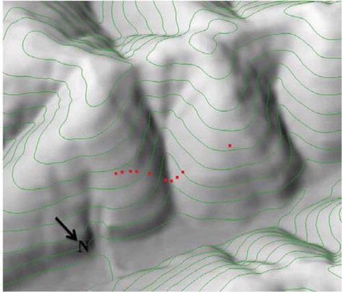
Figure 8. Locations of evaluation samples collected through regular sampling.

The targeted soil property to be predicted is soil organic matter (SOM) content (%) in top layer. Since the study area is fairly homogeneous in terms of macro-climate, parent materials and vegetation conditions, thus six topographic covariates (elevation, slope gradient, planform curvature, profile curvature, relative position index and topographic wetness index (TWI)) related to SOM content in the study area were used as covariates to characterize the geographic configuration. The micro-variation of other environmental conditions can be well represented by the topographic conditions (Zhu et al. 2008). It is noted here that the conditions of these covariates at a site constitute the geographic configuration for the site.

A 10 m resolution DEM created from the 1:10,000 topographic map of the area using the TOPOGRID and TINLATTICE in Arc/Info (Yang et al. 2007) was used to generate the slope gradient, contour curvature and profile curvature through 3DMapper (solim.geography.wisc.edu). TWI was calculated using the method proposed by Qin et al. (2011).

4.2. Methods of spatial predictions and evaluation

In this illustration, three methods of spatial prediction are used to generate the spatial variation of SOM (%). The first is the individual sample based predictive soil mapping method (iPSM), which is based on the Third Law of geography (Zhu et al. 2015a). The details of this approach and its implementation of the Third Law of Geography are beyond the scope of this discussion and interested readers are directed to Zhu et al. (2015a) for further reading. The following covariates: elevation, slope gradient, planform curvature, profile curvature, relative position index and TWI, were used to construct the geographic configuration for each location (whether sample point or prediction point). No spatial structure, nor hierarchy of variables will be used here for the simplicity of illustration. The prediction process of iPSM is as shown in Figure 5 and the similarity between a prediction point and sample point was calculated using Equation 4 shown below (Zhu et al. 2015a). For each location, a SOM value and an uncertainty value were computed.

(4) $S_{0,k}=\underset{m}{\overset{v=1}{P}}(E_v(e_{v,0},e_{v,k}))$(4)

where S_0,k represents the similarity between an prediction point (0) and a soil sample k; e_v,₀ and e_v,_k are the values of the v-th covariate at point (0) and at soil sample k, respectively; m is the number of selected covariates. Operator E_v is the function evaluating similarity between prediction point (0) and sample k based on v-th covariate and Operator P is the function which integrates the similarities based on individual covariates to create a final similarity between the two locations.

The second method is the multiple linear regression (MLR) representing the statistical principle. The independent variables are as the same as those listed for the iPSM method. A stepwise linear regression was used to avoid multi-collinearity among the six environmental covariates. The regression coefficients were estimated by Ordinary Least Squares (OLS) method using the 10 soil samples along the transect line. Only TWI and planform curvature were selected as predictors through stepwise analysis. The obtained regression was then applied to every location across the study area to compute the SOM value. No uncertainty value was produced with this method.

The third method is regression Kriging (RK) which represents the combination of the statistical principle and the First Law of Geography. RK is a widely used technique for spatial prediction due to its ability to utilize both the spatial relationship and the covariate relationship(s) (Hengl, Heuvelink, and Stein 2004). In this case study, the regression component of RK was that constructed for the MLR method as described above. The regression residuals at the 10 sample points on the transect were then used to construct a semivariogram to describe the spatial autocorrelation of the residuals and used in the Kriging component (e.g. ordinary Kriging) of RK. The regression component and the Kriging component are added together as the final RK model (Hengl, Heuvelink, and Rossiter 2007). For this model both the SOM value and the error variance for each location were computed. The error variance was regarded as the prediction uncertainty at each location.

Evaluation of the three methods was conducted in two aspects. First, the predication accuracy for each of the methods at the 44 evaluation points was calculated using the measures of Root Mean Squared Error (RMSE) and mean absolute error (MAE). The methods were compared on these two accuracy measures. The second aspect is the utility of prediction uncertainty, which only produced by iPSM and RK, in relation to prediction residuals at the 44 evaluation points. A positive relationship was expected if the prediction uncertainty was indicative of the prediction accuracy (i.e. the higher the prediction uncertainty, the higher prediction residual).

4.3. Prediction results

Figure 9(a) shows the predicted SOM content (%) map by iPSM, in which the predicted values range from 2.33% to 11.76%. Comparatively, Figure 9(b) shows the predicted SOM map by RK, in which, the predicted values of SOM content range from −40.89% to 25.98%. The unreasonable negative predicted values were assigned to ridges and valleys, which are the landscapes that cannot be represented by the 10 soil samples. On the predicted SOM content (%) map by iPSM (Figure 9(a)), the upper-to-middle steep slopes were assigned relatively low SOM content values while the lower-to-toe gentle slopes were assigned relatively high SOM content values. This spatial distribution pattern matches the knowledge on how slope position and slope gradient influence SOM content: on upper-to-middle steep slopes erosional processes tend to be the dominant processes which reduce the SOM content in the top soil layer; on lower-to-toe gentle slopes depositional processes tend to be the dominant processes which usually leads to higher SOM content in the top soil layer. In contrast, on the SOM content (%) map predicted by RK (Figure 9(b)), the values of SOM content at different slope positions with different slope gradient (e.g. upper-to-middle steep slope and lower to toe gentle slope) could not be well differentiated. This was mainly due to the fact that relative position index and slope gradient were not selected as predictors in the stepwise linear regression in the construction of the RK model.

Figure 9. Predicted top-layer SOM content (%) using (a) iPSM and (b) RK.

The prediction accuracies evaluated by 44 validation samples are listed in Table 1. Both the RMSE (6.095) and MAE (3.012) of RK are higher than those of iPSM (1.195 RMSE and 1.009 MAE). It is clear that the 10 sample points on a transect do not meet the requirement on sample size and sample distribution by the Kriging method and it is expected that the Kriging component of RK contributed little to the improvement of prediction accuracy. This is supported by the fact that there is no difference in RMSE and the MAE between RK and the MLR (Table 1).

Table 1. Prediction accuracy of iPSM, RK and MLR methods.

Method	RMSE	MAE
iPSM	1.195	1.009
RK	6.095	3.012
MLR	6.096	3.012

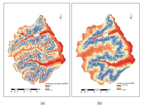
The prediction uncertainty using the iPSM method is shown in Figure 10(a). Since the 10 soil samples are mainly located on side slopes (Figure 7) and can represent those areas well, the prediction uncertainty is generally low in those areas. In contrast, high prediction uncertainty values were assigned to ridges and valleys because the 10 soil samples cannot represent those areas. Figure 10(b) shows the variance of errors computed in RK (i.e. RK variance), which is commonly used as a measurement of prediction uncertainty (Hengl, Heuvelink, and Stein 2004).

Figure 10. Prediction uncertainty produced by (a) iPSM and (b) RK.

The values of prediction uncertainty estimated from iPSM at the 44 validation sample locations were plotted against the corresponding prediction residuals in Figure 11. The dashed regression line with the correlation coefficient r (0.546) and the p-value of slope (0.000151) indicates a positive relationship between prediction uncertainty and prediction residual produced by iPSM. This implies that the prediction uncertainty estimated by iPSM can be used as an indicator to its prediction accuracy at each unvisited location.

Figure 11. The relationship between prediction uncertainty and prediction residual produced by iPSM.

The values of variance of errors estimated by RK at the 44 validation sample locations were plotted against the corresponding prediction residuals in Figure 12(a). Though a strong positive relationship was found (r = 0.931, p-value of slope <2e−16), it is mainly due to the two outlier points with extremely large RK variance and prediction residual. The majority of scatter plots did not show a very significant positive relationship. The removal of the two outliers resulted in the scatter plot in Figure 12(b) with r = 0.387 but the p-value of slope = 0.015. The results suggested that the prediction uncertainty estimated by the iPSM method was more effective in indicating prediction accuracy than that by the RK method.

Figure 12. The relationship between RK variance and RK prediction residual: (a) using all 44 validation samples, (b) using the validation samples without the two outliers in (a).

4.4. Observations

In the comparison between iPSM, which is based the Third Law of Geography, and RK, which is based the combination of First Law and the statistical principle, it might appear to be unfair to use RK with only 10 soil samples along a transect line, knowingly that these samples are not sufficient to construct the linear regression and the semivariogram. However, this is exactly the scenario why spatial prediction methods based on the Third Law of Geography are needed. This demonstrates that spatial prediction based on the Third Law is free of specific requirement on sample size and sample distribution, which make the existing samples collected in various ways possible to be used effectively in spatial prediction. This flexibility makes the spatial prediction based on the Third Law of Geography more suitable for large areas where a single and comprehensive sample set would be difficult to be collected at once but multiple, partial sample sets collected by different parties for different purposes are often available. In addition, samples collected through citizen science projects and provided through VGI can now be effectively used in spatial prediction under the Third Law of Geography.

It is also important to observe that the prediction uncertainty from iPSM is more informative than that of the RK. The improved ability of prediction uncertainty in relation to the quality of results from spatial prediction is a great asset since it offers an informative guidance as to where to sample to improve the prediction quality. This improved ability also helps to improve the effectiveness of uncertainty assessment (or sensitivity analysis) in geographic modeling.

5. Discussion

5.1. An invitation

This paper presents the idea of the Third Law of Geography and its implication for spatial prediction. A complete treatment on these two topics is almost impossible given the space available. However, our efforts here are to outline the essence of the Third Law of Geography, and how this essence changes the way spatial prediction can be conducted. Under this notion, Section 3 was devoted to present this essence and the theoretical basis for the shift in spatial prediction. The case study presented in Section 4 was to illustrate through an example how spatial prediction can be conducted based on the Third Law of Geography and to show the important differences in the use of samples between spatial prediction based on the Third Law of Geography and that based on the other principles. This case study is not here to validate the various impacts the Third Law of Geography could bring to spatial prediction, nor was it designed to compare and contrast the many differences between spatial predictions using the Third Law of Geography and other geographic principles (such as the First Law and the Second Law of Geography). These validations, comparisons and contrasts deserve separate and detailed treatments through additional studies. Thus, we use this paper as an invitation to explore the impacts of this important geographic principle in spatial prediction and in other geographic analysis.

5.2. The differences from the statistical principle used in spatial prediction

One may suggest that the Third Law of Geography is almost the same as the statistical principle used in spatial prediction. The differences between the two may not appear as apparently as one hopes at the beginning but the differences are significant. The first difference is that the Third Law of Geography calls for the comparison of geographic configurations at two locations. It does not relate the target variable to the set of covariates directly, nor does it demand an explicit relationship to be defined, but the statistical principle does. The second difference is that the Third Law stipulates the configuration of geographic conditions in examining the similarity of geographic environment at two points. This configuration contains the structure of the variables, not only the order of importance but also the combination effects of different variables in determining the value of target variable. The third difference is the spatial structure in comparison of the geographic configurations. It calls for the geographic conditions over certain size of areas to be included in this comparison which could be considered in the statistical principle when applied to spatial prediction but it more than often is not.

5.3. Differences from the First Law and the Second Law of Geography

The three laws of geography examine different aspects of the complexity of geography reality. The Third Law of Geography explores the use of similarity in geographic configuration (structure of variables and spatial foot print) while the First Law and the Second Law examines the variation over distance (spatial correlation by the First Law and spatial heterogeneity by the Second Law). The other difference is that the First and Second Laws focus on geographic similarity or differences based on one variable, that is spatial distance, while the Third Law focuses on the similarity in the configuration of many geographic variables. In some way, the First Law and the Second Law could be seen as the special cases of the Third Law.

In their applications to spatial prediction, the Third Law relaxes the constraints imposed by the First Law and the Second Law by allowing the representativeness of a single sample to be explicitly used in spatial prediction. There is no need for the quantification and expression of explicit relationships, and thus the requirement on sample size and sample distribution, which is an important condition of spatial prediction based on the First Law and the Second Law as well as the statistical principle, can be avoided. Clearly, the use of a single sample point does have its cost since a single sample point does not have the degree of freedom to check itself for the information it contains as well as the relationship it represents. Efforts are under way to quantify the reliability of a single sample point when using it in spatial prediction (Liu 2017; Liu, et al., under review).

The uncertainty computed based on the representativeness of a sample point to a prediction point as expressed in similarity between the geographic configuration of the sample and that of the prediction point is extremely useful not only in assessing the quality of the results from spatial prediction but also in allocating error reduction efforts (Zhang et al. 2016; Li et al. 2016). This uncertainty is different from the error variance of prediction from the Kriging family of models in that the Kriging family of methods report the error variance of prediction due to the spatial distribution of samples while the uncertainty computed based on the Third Law measures how well the various geographic configurations in the study area have been represented by the configurations already captured by the sample points. It directly assesses the sufficiency of samples in capturing the spatial variability of the study area.

6. Conclusion

This paper presents an important geographic principle, referred to as the Third Law of Geography, in the context of spatial prediction. This new principle (law) provides a new way how spatial prediction can be conducted, which is fundamentally different from those based on other principles (namely the First Law, the Second Law of Geography and the statistical principle). The key differences are: 1) the use of comparison of geographic configuration, rather than the explicit extraction of relationships; 2) the use of representativeness of a single sample point, rather than the average representation of a sample set.

In summary, spatial prediction based on the Third Law of Geography has the following properties: 1) no specific requirement on the distribution nor the size of sample set, 2) the use of a single sample point for capturing representation to the study area, and 3) the uncertainty measure expressing the coverage of the various geographic configurations. These properties make spatial prediction more suitable for estimating spatial variation of geographic variables over areas of complex geographic reality in terms of samples required, uncertainty provision as well as guidance to error reduction efforts.

Acknowledgements

The work reported here was supported by grants from National Natural Science Foundation of China (Project No.: 41431177), National Basic Research Program of China (Project No.: 2015CB954102), PAPD, and Outstanding Innovation Team in Colleges and Universities in Jiangsu Province. Supports to A-Xing Zhu through the Vilas Associate Award, the Hammel Faculty Fellow Award, and the Manasse Chair Professorship from the University of Wisconsin Madison are greatly appreciated. We also greatly appreciate the detail reviews and the helpful comments from the two reviewers.

Disclosure statement

No potential conflict of interest was reported by the authors.

References

- Anselin, L. 2013. Spatial Econometrics: Methods and Models (Vol. 4). New York, NY: Springer Science & Business Media.
- Brunsdon, C., A. S. Fotheringham, and M. E. Charlton. 1996. “Geographically Weighted Regression: A Method for Exploring Spatial Nonstationarity.” Geographical Analysis 28: 281–298. doi:10.1111/j.1538-4632.1996.tb00936.x.
- Cressie, N. 1991. Statistics for Spatial Data, 900 pp. New York, NY: Wiley.
- Cruden, D. 2017. Landslide Risk Assessment. London: Routledge.
- Dokuchaev, V. V. 1883/1948/1967. “Russian Chernozem.” In Selected Works of V. V. Dokuchaev, Moscow, 1948, 1, 14–419, (for USDA-NSF), Publ. by S. Monson, 1967. (Transl. into English by N. Kaner). Jerusalem: Israel Program for Scientific Translations.
- Eldawy, A., and M. F. Mokbel, 2015. The Era of Big Spatial Data. In: Data Engineering Workshops (ICDEW), The 31st IEEE International Conference, 42–49. Doi:10.1177/1753193414554357
- Fotheringham, A. S., and C. Brunsdon. 1999. “Local Forms of Spatial Analysis.” Geographical Analysis 31: 340–358. doi:10.1111/j.1538-4632.1999.tb00989.x.
- Fotheringham, A. S., C. Brunsdon, and M. Charlton. 2002. Geographically Weighted Regression - the Analysis of Spatially Varying Relationships. Chichester: Wiley.
- Goodchild, M. F. 2004a. “GIScience: Geography, Form, and Process.” Annals of the Association of American Geographers 94: 709–714.
- Goodchild, M. F. 2004b. “The Validity and Usefulness of Laws in Geographic Information Science and Geography.” Annals of the Association of American Geographers 94: 300–303. doi:10.1111/j.1467-8306.2004.09402008.x.
- Goodchild, M. F. 2007. “Citizens as Sensors: The World of Volunteered Geography.” GeoJournal 69 (4): 211–221. doi:10.1007/s10708-007-9111-y.
- Goodchild, M. F., and A. J. Glennon. 2010. “Crowdsourcing Geographic Information for Disaster Response: A Research Frontier.” International Journal of Digital Earth 3 (3): 231–241. doi:10.1080/17538941003759255.
- Goodchild, M. F., B. O. Parks, and L. T. Steyaert, eds. 1993. Environmental Modeling with GIS. New York, USA: Oxford University Press.
- Goodchild, M. F., L. T. Steyeart, and B. O. Parks. 1996. GIS and Environmental Modeling: Progress and Research Issues. GIS World:Fort Collins, USA.
- Goovaerts, P. 1999. “Geostatistics in Soil Science: State-Of-The-Art and Perspectives.” Geoderma 89 (1–2): 1–45. doi:10.1016/S0016-7061(98)00078-0.
- Haklay, M. 2013. “Citizen Science and Volunteered Geographic Information: Overview and Typology of Participation.” In Crowdsourcing Geographic Knowledge, edited by D. Sui, S. Elwood, and M. Goodchild. Dordrecht: Springer.
- Hartshorne, R. 1939. “The Nature of Geography: A Critical Survey of Current Thought in the Light of the Past.” Annals of the Association of American Geographers 29 (3): 173–412. doi:10.2307/2561063.
- Hartshorne, R. 1959. Perspective on the Nature of Geography. Chicago: Rand McNally.
- Harvey, D. 1996. Justice, Nature and the Geography of Difference. Oxford: Basil Blackwell.
- Hengl, T., G. B. M. Heuvelink, and A. Stein. 2004. “A Generic Framework for Spatial Prediction of Soil Variables Based on Regression-Kriging.” Geoderma 120: 75–93. doi:10.1016/j.geoderma.2003.08.018.
- Hengl, T., G. B. M. Heuvelink, and D. G. Rossiter. 2007. “About Regression-Kriging: From Equations to Case Studies.” Computers & Geosciences 33 (10): 1301–1315. doi:10.1016/j.cageo.2007.05.001.
- Hunsaker, C. T., M. F. Goodchild, M. A. Friedl, and T. J. Case, Eds.. 2013. Spatial Uncertainty in Ecology: Implications for Remote Sensing and GIS Applications. Springer Science & Business Media, New York.
- Isaaks, E. H., and R. M. Srivastava. 1989. An Introduction to Applied Geostatistics. New York, NY: Oxford University Press.
- Jenny, H. 1994. Factors of Soil Formation: A System of Quantitative Pedology. North Chelmsford, MA: Courier Corporation.
- Kanevski, M., V. Timonin, and A. Pozdnukhov. 2009. Machine Learning for Spatial Environmental Data: Theory, Applications, and Software. Lausanne: EPFL Press.
- Kitanidis, P. K., and K. F. Shen. 1996. “Geostatistical Interpolation of Chemical Concentration.” Advances in Water Resources 19 (6): 369–378. doi:10.1016/0309-1708(96)00016-4.
- Krige, D. G. 1951. “A Statistical Approach to Some Basic Mine Valuation Problems on the Witwatersrand.” Journal of the Chemical, Metallurgical and Mining Society of South Africa 52 (6): 119–139.
- Li, J., A. D. Heap, A. Potter, and J. J. Daniell. 2011. “Application of Machine Learning Methods to Spatial Interpolation of Environmental Variables.” Environmental Modelling & Software 26 (12): 1647–1659. doi:10.1016/j.envsoft.2011.07.004.
- Li, Y., A. X. Zhu, Z. Shi, J. Liu, and F. Du. 2016. “Supplemental Sampling for Digital Soil Mapping Based on Prediction Uncertainty from Both the Feature Domain and the Spatial Domain.” Geoderma 284: 73–84. doi:10.1016/j.geoderma.2016.08.013.
- Ließ, M., B. Glaser, and B. Huwe. 2012. “Uncertainty in the Spatial Prediction of Soil Texture: Comparison of Regression Tree and Random Forest Models.” Geoderma 170: 70–79. doi:10.1016/j.geoderma.2011.10.010.
- Liu, J., 2017. Integration of Samples from Multiple Sources for Predictive Mapping over Large Areas, PhD thesis, University of Wisconsin – Madison, Madison, WI, USA.
- Liu, J., A. X. Zhu, D. Rossiter, F. Du, and J. Burt. 2018. “Reliability Estimation of Individual Sample Points in Individual Predictive Soil Mapping (Manuscript under Review).”
- Matheron, G. 1963. “Principles of Geostatistics.” Economic Geology 58: 1246–1266. doi:10.2113/gsecongeo.58.8.1246.
- Miller, D. A., and R. A. White. 1998. “A Conterminous United States Multilayer Soil Characteristics Dataset for Regional Climate and Hydrology Modeling.” Earth Interactions 2 (2): 1–26. doi:10.1175/1087-3562(1998)002<0001:ACUSMS>2.3.CO;2.
- Odeh, I. O., A. B. McBratney, and D. J. Chittleborough. 1995. “Further Results on Prediction of Soil Properties from Terrain Attributes: Heterotopic Cokriging and Regression-Kriging.” Geoderma 67 (3–4): 215–226. doi:10.1016/0016-7061(95)00007-B.
- Phillips, J. D. 2003. “Sources of Nonlinearity and Complexity in Geomorphic Systems.” Progress in Physical Geography 27: 1–23. doi:10.1191/0309133303pp340ra.
- Qin, C.-Z., A.-X. Zhu, T. Pei, B.-L. Li, T. Scholten, T. Behrens, and C.-H. Zhou. 2011. “An Approach to Computing Topographic Wetness Index Based on Maximum Downslope Gradient.” Precision Agriculture 12 (1): 32–43. doi:10.1007/s11119-009-9152-y.
- Shi, W. 2008. “Modeling Uncertainty in Geographic Information and Analysis.” Science in China Series E: Technological Sciences 51 (1): 38–47. doi:10.1007/s11431-008-5019-0.
- Skidmore, A., eds.. 2003. Environmental Modelling with GIS and Remote Sensing. Boca Raton, FL: CRC Press.
- Stein, A., and L. Corsten. 1991. “Universal Kriging and Cokriging as a Regression Procedure.” Biometrics 47 (2): 575–587. doi:10.2307/2532147.
- Sui, D., S. Elwood, and M. Goodchild, eds.. 2012. Crowdsourcing Geographic Knowledge: Volunteered Geographic Information (VGI) in Theory and Practice. New York, NY: Springer Science & Business Media.
- Tobler, W. R. 1970. “A Computer Movie Simulating Urban Growth in the Detroit Region.” Economic Geography 46 (sup1): 234–240. doi:10.2307/143141.
- Tomlinson, R. F., H. W. Calkins, and D. Marble. 1976. Computer Handling of Geographic Data: An Examination of Selected Geographic Information Systems. Paris,: UNES.
- Van Westen, C. J., E. Castellanos, and S. L. Kuriakose. 2008. “Spatial Data for Landslide Susceptibility, Hazard, and Vulnerability Assessment: An Overview.” Engineering Geology 102 (3–4): 112–131. doi:10.1016/j.enggeo.2008.03.010.
- Wingle, W. L., and E. P. Poeter. 1998. “Directional Semivariograms: Kriging Anisotropy without Anisotropy Factors.” Advances in Geostatistics 2: 1–4.
- Wortley, R., and M. Townsley, eds.. 2016. Environmental Criminology and Crime Analysis. Vol. 18. London: Taylor & Francis.
- Yang, L., A. X. Zhu, B. L. Li, C. Z. Qin, T. Pei, B. Y. Liu, R. K. Li, and Q. G. Cai. 2007. “Extraction of Knowledge about Soil-Environment Relationship for Soil Mapping Using Fuzzy C-Means (FCM) (In Chinese).” Acta Pedologica Sinica 44 (5): 784–791.
- Zhang, S. J., A. X. Zhu, J. Liu, C.-Z. Qin, and Y.-M. An. 2016. “An Heuristic Uncertainty Directed Field Sampling Design for Digital Soil Mapping.” Geoderma 267: 123–136. doi:10.1016/j.geoderma.2015.12.009.
- Zhu, A. X., L. Yang, B. Li, C. Qin, E. English, J. E. Burt, and C. H. Zhou. 2008. “Purposefully Sampling for Digital Soil Mapping.” In Digital Soil Mapping with Limited Data, eds A. E. Hartemink, A. B. McBratney, and M. L. Mendonca Santos, 233–245. New York: Springer-Verlag.
- Zhu, A. X., G. M. Zhang, W. Wang, W. Xiao, Z. P. Huang, D. Z. Ge-Sang, G. P. Ren, et al. 2015b. “A Citizen Data-Based Approach to Predictive Mapping of Spatial Variation of Natural Phenomena.” International Journal of Geographical Information Science 29 (10): 1864–1886. doi:10.1080/13658816.2015.1058387.
- Zhu, A. X., J. Liu, F. Du, S. J. Zhang, C. Z. Qin, J. Burt, and T. Scholten. 2015a. “Predictive Soil Mapping with Limited Sample Data.” European Journal of Soil Science 66 (3): 535–547. doi:10.1111/ejss.12244.