Evaluation of landslide susceptibility in a hill city of Sikkim Himalaya with the perspective of hybrid modelling techniques

ABSTRACT

Landslides are common and frequent occurring phenomenon in hilly terrain during monsoon season. The primary objectives of the research work are to carry out a comprehensive analysis by quantifying the landslide susceptibility using an integrated approach of random forest (RF) with the probabilistic likelihood ratio (RF-PLR), fuzzy logic (FL) and index of entropy (IOE) in Gangtok city of Sikkim state, India. Landslide inventories are prepared based on LISS-IV (MX) satellite imagery, Google Earth and reported data of Geological Survey of India. Altogether 12 landslide conditioning factors viz. slope, elevation, curvature, aspect, land use/land cover, geology, lineament, rainfall, soil type, soil thickness, water regime and distance from road are considered as input data for geospatial modelling of landslide susceptibility. Finally, model-derived landslide susceptibility maps are classified into four hazard zones, i.e. low, medium, high and very high. To measure model compatibility model comparison is performed in ArcGIS environment and models performance is assessed by confusion matrix where RF-FL gives more accuracy of 69.36% than other two models with 9.68% and 19.35% of Type I and type II error, respectively. The outputs are validated using success and prediction rate method where, RF-PLR, RF-FL and RF-IOE show area under curve (AUC) of success and prediction rate as 76%, 67%, 83%, 78% and 85%, 80%, respectively. Additionally, the differences in model performances were analyzed by means of Wilcoxon signed rank test, where it was found that statistically differences in the performance was significant in case of RF-PLR vs. RF-FL and RF-PLR vs. RF-IOE.

KEYWORDS:

• Landslide susceptibility
• Gangtok
• Sikkim Himalaya

Introduction

Sikkim Himalaya faces numerous landslides per year resulting in thousands of fatalities (Bhasin et al. 2002). In Sikkim, about 36,000 people were killed by landslides (Choubey 1992) in 1968 alone. There are many factors that are responsible for slope instability, but the main controlling factors are rainfall, seismic activities and anthropogenic activities (Lin et al. 2006; van Westen, Castellanos, and Kuriakose 2008; Gupta et al. 2018; Zhang et al. 2018). Therefore, landslide susceptibility mapping is very important for disaster prevention and mitigation guide. These maps can be quantitative or qualitative (Soeters and van Westen 1996; Guzzetti et al. 1999). In the late 1970s, qualitative methods were widely used by researchers. In the last few decades, quantitative methods which are based on the relationship between landslide occurrence and controlling factors become popular (van Westen, Rengers, and Soeters 2003, 2008; Glade and Crozier 2005; Chen and Wang 2014; Kannan, Saranathan, and Anbalagan 2015; Samia et al. 2018). Landslide susceptibility is the key component of landslide hazard and risk assessment, and land use planning. Landslide susceptibility is a time-invariant concept that defines the probability of landslide occurrence in an area based on a set of controlling factors, i.e. geology, slope, land use land cover, etc. (Brabb 1984; Guzzetti et al. 2005). Therefore, landslide susceptibility is dissimilar from landslide hazard because landslide hazard considers the temporal probability of landslide occurrences and its magnitude (Guzzetti et al. 2005).

Landslide susceptibility zonation has been carried out widely all around the world to demarcate landslide vulnerable areas using remote sensing and Geographical Information System (Anbalagan et al. 2015; Kannan, Saranathan, and Anbalagan 2015). Landslide susceptibility mapping is done by two process namely qualitative (knowledge-driven) and quantitative (statistical) techniques (Kaur et al. 2017a). Expert knowledge develops through a combination of field experiences and theoretical understanding of physical processes. In knowledge-driven model the complicated non-linear relationship between landslide susceptibility and landslide causing factors are extracted by assigning weight to the factors based on expert knowledge (Zhu et al. 2014; Pathak 2016). The success of knowledge-driven model is mainly based on expert knowledge (Kaur et al. 2017; Gupta et al. 2018). There are various reported studies on comparative study of an expert knowledge-based model and data-driven models for landslide susceptibility mapping (Zhu et al. 2014, 2018; Kavzolu, Colkesen, and Sahin 2019). Quantitative analysis or statistical models determine weight and rank based on logical tools but these statistical models require more data to generate a reliable result (Tien Bui et al. 2011; Kaur, Gupta, and Parkash 2017a; Chen et al. 2018). To overcome this issue, machine-learning techniques such as decision trees (Dietterich 2000; Althuwaynee et al. 2014; Hong et al. 2018), neuro-fuzzy (Pradhan, Lee, and Buchroithner 2010), support vector machines (Chen et al. 2017a; Tien Bui et al. 2017), boosted regression trees (Youssef et al. 2016; Lee et al. 2017), kernel logistic regression (Tien Bui et al. 2016; Chen et al. 2017b), naive bayes (Tsangaratos and Ilia 2016; Tien Bui et al. 2017) and random forests (RF) (Pourghasemi and Kerle 2016; Kim et al. 2018; Zhang et al. 2017; Chen et al. 2018) are widely used throughout the globe. In recent year’s, comparison between different models are being widely used to determine the best techniques for landslide susceptibility zonation (Ciurleo, Cascini, and Calvello 2017; Chen et al. 2018). According to Chen et al. (2018), hybrid approach by integrating two or more models such as artificial neural network combined with fuzzy logic (Kanungo et al. 2009), adaptive neuro-fuzzy inference (Dehnavi et al. 2015), ANFIS integrated with combined FR (Chen et al. 2017), random forest combined with statistical index (Chen et al. 2018), random forest with index of entropy (Chen et al. 2018) gives a better result with reasonable conclusion. Performance of such models is usually assessed with receiver operating characteristic (ROC) curves, success and prediction rate curves (SPRC) and area under curve (AUC) values.

With this background, some hybrid techniques such as random forests and probabilistic likelihood ratio (RF-PLR), fuzzy logic (FL) and index of entropy (IOE) are developed integrated with machine-learning model RF. This technique is used in the present study in order to remove the subjectivity, unevenness and realistic result of the models. Probabilistic likelihood ratio (PLR) approach deals with real landslide data in determining the rate without considering the relativity whereas fuzzy logic (FL) develops the concept of relativity in rate determination and index of entropy (IOE) remove the unevenness among the conditioning factors.

The present study is conducted with the objectives to determine the weight and ranks for each factors class and their subclass respectively using PLR, fuzzy membership and IOE techniques and to combine the PLR, FL and IOE derived results with RF with a view to generate best susceptibility output for the study. The importance of the conditioning factors is calculated by RF. So far, this technique is not used to generate LSZ for the Gangtok city. Model-generated outcomes are also corroborated with respect to geology and social vulnerability of the study area. The outcomes of the present research will be helpful towards landslide risk reduction and highlighting the applicability of hybrid statistical technique-based susceptibility modelling in the Gangtok city through the proper understanding of landslide conditioning factors. This study can also be opened up as a possible way for landslide studies in hill city, Gangtok in the eastern Himalayas, as well as for western Himalayas, Nilgiri and Nepal Himalayas.

Study area

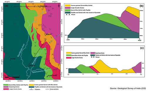
Gangtok, geographically bounded by 27.3325°N latitude to 88.6140°E, longitude is situated at an altitude of about 1800 m above sea level encompassing the third highest mountain (Mount Kanchenjunga) in the World. Gangtok city is flanked by two rivers, i.e. Rorochu in the eastward side and Ranikhola on the west. Both the rivers meet at Ranipool and flow towards the south before they again join the Teesta at Singtam. The city is located at the south-facing slope of Eastern Himalaya and has erosional topography bounded and dissected by a large number of perennial and seasonal springs. The study area experiences a high variation of rainfall throughout the year (Figure 1) with maximum daily rainfall reaches up to several hundred mm (Bhasin et al. 2002). Several rainfall triggered landslide events were reported in the study area (Ghosh et al. 2016; Rawat 2005; Bhasin et al. 2002). The East district is the most populated and urbanized among the four districts (North, South, East and West) of Sikkim, sharing 79.55% of the total urban population. The rising trend of urbanisation in East district is mainly concentrated at the capital city of Gangtok and its surrounding areas and puts tremendous pressure in the study area thereby accelerates the chance of landslides (both natural and anthropogenic) associated which greater loss of lives and properties (Kaur et al. 2018). For the city, 7 June 1997 is often referred as a ‘black day’ since in this particular date, the city had witnessed a number of landslides due to heavy rainfall (approximately 224 mm) causing more than 50 fatalities, 60 people injuries, more than 5000 people lost their home and disruption of National Highway 31A (near Rangpo town). Incessant rainfall on 27 June 2007 caused a landslide in the Taktse area of Bojhoghari in Gangtok, resulting in washed away of houses. In the aftermath of 18 September 2011, Sikkim earthquake triggered several landslides in the city causing several causalities and loss of properties (Chakraborty et al. 2011). This study is carried out within 17 wards of Gangtok town, encompassing an area of 19.345 km² (Table 1). Figure 2 shows the location of the study area. Geologically, Gangtok rests over coarse-grained garnet mica schist of Daling group of rocks flanked by two thrust contacts (Figure 3). Detailed description of geology, geomorphology and hydrology related to study area is described in methodology section.

Table 1. Wards of GMC area.

Ward no.	Ward name	Area (km^2)	Population
01	*Burtuk	4.245	9,957
02	*Lower Sichey	3.083	5,873
03	Upper Sichey	0.681	7,979
04	Chandmari	2.911	6,177
05	Development Area	0.710	6,723
06	Diesel Power House (DPH)	0.212	3,987
07	Arithang	0.353	8,212
08	Lower M. G. Marg	0.142	4,032
09	Upper M. G. Marg	0.133	2,664
10	Tibet Road	0.329	3,266
11	Deorali	0.313	6,938
12	Daragoan	1.600	9,605
13	Tadong	1.250	9,325
14	Ranipool	1.217	4,520
15	Tathangchen Syari	2.166	11,028
Total area of GMC		19.345	100,286

*At present Burtuk and lower Sichey is divided into two wards each

Figure 1. Annual rainfall in Gangtok for the period of 2006–2017 (Source: Indian meteorological department).

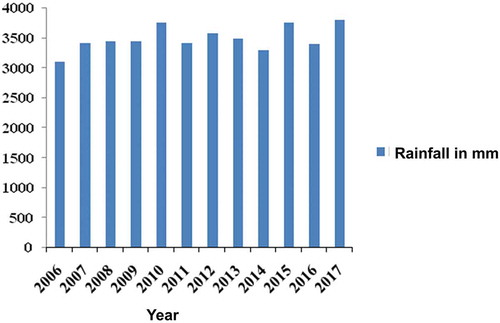
Figure 2. Location map of the study area.

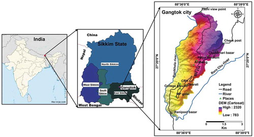
Figure 3. (a) Geological map of the Gangtok and its surrounding area, (b) cross-section along A-B line, (c) cross-section along C-D line.

Methodology

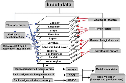
Landslides are generally controlled by several factors such as geology, slope morphology, soil, moisture conditions, rainfall, ground conditions, etc. (Ohlmacher 1930; Hong, Adler, and Huffman 2007). In the present study, 12 landslide influencing factors being categorized into geological, terrain, geomorphological and hydrological factors are considered as input parameters on the basis of review of literature and data availability (Bhasin et al. 2002; Sharma 2008; Ghosh et al. 2016; Kaur, Gupta, and Parkash 2017a; Kaur et al. 2018). The specifications of all the data used for modelling are represented in Table 2. All input data are converted into raster format with 20 × 20 m grid cell size and an area of 256 column and 455 rows to carry out further modelling. Figure 4 represents the detailed flowchart of the methodology adopted in carrying out the present research work.

Table 2. Data used in the present study.

Data type	Date and year	Scene timing	Sensor	Resolution	Space agency
Resourcesat-2	4–12-2006	Start time: 04:52:07:076	Multispectral (LISS-IV)	5 m	Indian Space Research Organization (ISRO)
		End time: −
		Centre time: 04:52:17:738
	20–11-2011	Start: 04:48:05:023
		End: 04:48:15:077
		Centre: 04:48:10:050
	17–11-2016	Start: 04:54:57:032
		End: 04:55:07:086
		Centre: 04:55:02:059
Google Earth Pro	2010–2015	–	–	15 m to 15 cm	US Department of State Geographer
Reported Data	1975–2013	–	–	–	Geological Survey of India (GSI)

Figure 4. Work flow of methodology adopted.

Landslide incidence map

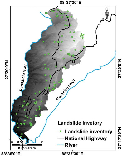
Landslide occurrence is based on the principle that ‘slope failure are more likely to occur under a condition that led to past instability’ (Guzzetti et al. 2000). So, it is important to trace past landslides for the prediction of future landslide occurrences. In landslide studies, past data are used to prepare the inventory. Generally, two types of inventory are developed for landslide susceptibility zonation, i.e. landslide inventory map (Basharat, Shah, and Hameed 2016; Kaur et al. 2018) and event landslide inventory map (Guzzetti et al. 2012; Mondini et al. 2014). Landslide inventory map shows the location and spatial extent whereas event landslide inventory indicates the extent, location and typology of landslide hazard caused by triggering factors. Landslide inventory is prepared from Resourcesat-2, Google Earth (Figure 5) and GSI reported data (Table 2). Resourcesat-2 and Google Earth imagery are used to identify the extent of landslide boundaries. Identifying minor or shallow landslide from satellite images is very difficult as the study area falls under Himalayan terrain with very high vegetated terrain. Past landslide data (1968–2013) are collected from the Geological Survey of India (Government Nodal Agency for landslide assessment). A total of 95 shallow landslide points are considered as landslide inventory (90 landslides are rainfall-induced and 5 landslides are related to 2011 Earthquake) (Supplementary Table 1). Figure 6 shows the location (centroid) of the landslide in the study area. The total landslide data are randomly splitted into two groups, i.e. training dataset (71 points) and testing dataset (24) (Althuwaynee, Pradhan, and Lee 2012; Neuhauser, Damm, and Terhorst 2012). Training data are used to develop the LSZ model whereas testing data are employed to validate the model (Chen et al. 2016).

Figure 5. Showing landslide scars in study area detected by LISS IV (left side) and google earth pro (right side).

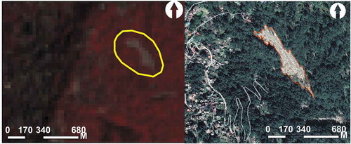
Figure 6. Landslide inventory map of the study area.

Landslide conditioning factors

Geology/lithology

The study area mostly consists of gneissic rocks (Lingtse granite and Darjeeling gneiss) and schistose rocks (mica schist, quartzite) type. Due to high rainfall, rocks are highly weathered and eroded at many places which causes frequent landslides. Detailed geology (1:25,000 scale) of the study area reveals various kinds of rock type viz. Darjeeling gneiss, coarse-grained garnet mica schist, garnet mica schist with phyllite, phyllite and schist with inter-bands of quartzite and Lingtse granite gneiss (Figure 7(a)). Arithang ward, development area and part of Sichey ward of GMC town are mostly occupied by high-grade streaky tourmaline biotite gneiss (Lingtse granite). The mica schist of the study area is coarse to very coarse-grained rock, mostly equigranular and almost monomineralic. The major constituents of mica schist rock are quartz (SiO₂), muscovite (KAl₂(SI₃Al)O₁₀(OH,F)₂), biotite (K(Mg,Fe)₃AlSi₃O₁₀(H,OH)₂), etc. with or without prophyroblasts of garnet, staurolite and kyanite. This type of rocks are mainly found in lower Burtuk, DPH (diesel power house), Tibet road, parts of upper Burtuk wards and north of Sichey ward. Quartzite occurs as an impersistant band within the phyllite and mica schist rock. The bands are usually found broken into rectangular blocks and in a few cases involved in the formation of boundinage. Quartzite bands are mostly exposed to the south of Tathangchen area, Tadong, Ranipool and Daragoan wards. Darjeeling gneiss formation is found in Chandmari, towards NE of Development area and upper Burtuk ward of GMC town.

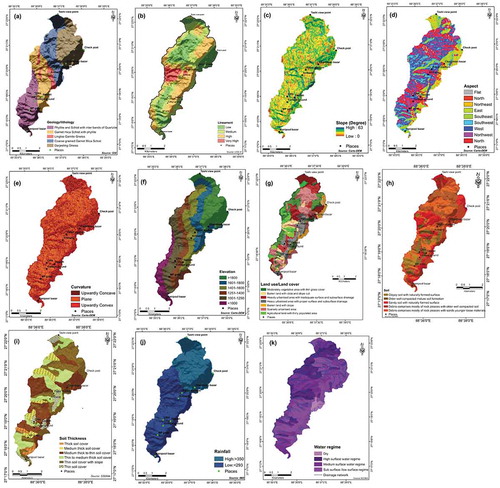
Figure 7. Input factors map (a) geology/lithology, (b) lineament, (c) slope, (d) slope aspect, (e) curvature, (f) elevation, (g) LULC, (h) soil, (i) soil thickness, (j) rainfall, (k) water regime.

Lineament density

Lineaments play a vital role in slope failure (Ramli et al. 2010). Lineaments describe the plane/zone of weakness and most landslides can occur at this weaker zone (Kannan et al. 2013; Thapa et al. 2017a). A regional lineament map is developed from IRS LISS III digital data (5 m resolution). Figure 7(b) shows the lineament density map prepared from lineaments extracted from satellite images. The distance from a lineament is calculated from Euclidean distance in ArcGIS environment, where proximity to lineament density is classified into four major classes namely low, medium, high and very high. The majority of large lineaments follow a NE-SW to ENE-WSW trend, whereas small lineaments mostly follow an E-W trend. There are also lineaments with N-S and NW-SE trends. Sichey ward in the western side of Gangtok town falls under the high lineament density class.

Terrain factors

Slope angle, aspect, curvature and elevation are the four most crucial causative terrain factors considered for the present study. They are extracted from CartoDEM (25 m resolution) and analyzed by ArcGIS surface analyst tools. Slope angle is the degree of change in elevation. The slope of the study area varies from 0° to 63° and is classified into flat (0–19°), moderate (20–39°), steep (40–59°), very steep (<60°) by natural jenks process (Figure 7(c)). Most of the study area belong to moderate slope with limited steep slopes. Gentle slopes are found on several river terraces and sometimes on accumulated slide debris. The slope aspect has been referred to compass directions which coincide with the geographic direction and varies from 0° to 360°. Aspect of the study area is classified into nine classes (flat, north, northeast, east, south-east, south, south-west, west and north-west) (Figure 7(d)). Curvature is the important preparatory factor to landslide susceptibility study as it affects the driving and resisting stress within a landslide in the direction of motion and controls the water in the landslide direction motion and convergence or divergence of landslide material (Carson and Kirkby 1972; Meten, Bhandary, and Yatabe 2015). Figure 7(e) represents various types of curvature patterns existing in the study area. In most of the landslide-related studies, elevation is considered as an indirect factor associated with other factors like rainfall, geology, soil, etc. The elevation of the study area varies from 783 m at south and 2320 m at north (Figure 7(f)) and the altitude of the study area is gradually higher in the northeast region. More than 70% of the area lies between 1000 and 1500 m altitudes. Several researchers (Dai and Lee 2002; Dragicevi, Lai, and Balram 2015; Wang et al. 2015) observed that landslides mostly occur at the intermediate range of elevation since slopes tend to be covered with a thin layer of colluviums which is vulnerable to landslides. ‘Distance (m) from road’ map is prepared by means of multiple buffering at a distance of 2000–6000 m with the help of ArcGIS software.

Morphological parameters

Land use and land cover (LULC) is an important factor to study the destabilization of slope (Mathew, Jha, and Rawat 2007). The presence of vegetation makes slope stable by better bonding with rock materials. Thus, slope with dense vegetation is more stable compared to barren land (Gentile, Elia, and Elia 2010). Vectorization processes are used to create land use and land cover maps (Kiran, Srivastava, and Jagannadha Rao 2014) over the GMC area. This process involves vector coverage of settlements, agricultural and forest areas. LULC map is prepared through visual interpretation of LISS IV images (4/12/2006, 20/11/2011 and 17/11/2016), Quickbird (0.6 m resolution) and Sikkim State Disaster Management Authority (SSDMA 2012) thematic map and later on the interpretations are confirmed during the field survey. Altogether seven different classes of LULC are identified and mapped namely sparsely urbanized areas, barren land with slope, heavily urbanized areas with proper surface and subsurface drainage, heavily urbanized areas with inadequate surface and subsurface drainage, barren land with slide and slope cut, moderately vegetative areas with thin grass cover and agricultural land with thiny populated areas (Figure 7(g)). Heavy urban agglomeration is predominantly found along Paljor stadium, Mahatma Gandhi Marg, Arithang, Deorali, MP Golai, Central Referral hospital (CRH) and Ranipool area. Agricultural land with thinly populated areas account for 1.65 km² (8.57%) of the area and is found in Tadong, Ranipool, Daragaon, lower Sichey-I and lower Burtuk wards of Gangtok town. Apart from these, barren lands with slide occupy 1.69 km² (8.77%) of the area. However, pine tree plantation has observed within the urbanized area between SNTM hospital to Zero point. In addition to pine plantation, bamboo trees also occur as wild growth in certain parts of Tathangchen ward (near Ridge Park). The cultivated patches are mostly seen in the thickly populated lower slope of Tathangchen, Burtuk, Development area, Tadong and Ranipool wards of Gangtok city.

Soil properties and soil thickness are important factors for slope stability (Champati Ray et al. 2007). Slope stability depends on soil texture as it influences the porosity and permeability of the soil. The study area soil mostly forms from gneissic and schistose group of rocks. The soil type and soil thickness maps of the study area are derived from SSDMA thematic maps. Transported and residual soils are the two categories of soil formed in the study area. In the present study area, soil type is categorized into five major classes viz., debris comprises mostly of rock pieces mixed with sands younger loose materials, debris comprises mostly of rock pieces along with older sand, sandy soil with the naturally formed surface, older well-compacted mature soil formation and clayey soil with a naturally formed surface (Figure 7(h)). Areas such as MP Golai, Lumsey and Chinten Bhavan consist of older well-compacted soil whereas clay soil is found near Adam pool, lower Siechey ward and some area of Deorali and Arithang ward. The area near Ranipool bazar, Palzor stadium, Chandmari bazar, balwakhan area of Burtak ward is characterized by debris soil which comprises mostly of rock pieces and older well-compacted sands. Debris with younger loose sand type is found in nearby places of Holly cross school and Secretariat. Sandy soil with the naturally formed surface is found in the Sichey ward, Tashi view point, Bojoghari and check post of Chandmari ward. Soil thickness of the Gangtok region is classified into six classes namely thin soil cover, thin soil cover with slope, thin to medium thick soil cover, medium thick to thin soil cover, medium thick soil cover and thick soil cover (Figure 7(i)). Approximately 7.03 km² area is covered by thin soil cover with or without slope. Medium thick soil to thick soil covers an area of 7.34 km².

Hydrological factors

Gangtok region receives an average annual rainfall of 3429 mm. The months from June to September are characterized by intense rainfall. July has the highest monthly average rainfall of about 649.6 mm (India Meteorological Department 2007). Figure 7(j) represents the spatial distribution of the rainfall in the study area.

It is an important feature to measure slope stability as it determines the frictional force and pore pressure of the study area. The water regime map is prepared based on the drainage pattern of the study area. The present study area is divided into four categories of water regime, i.e. sub-surface/low surface water regime, medium surface water regime, high surface water regime and dry surface water regime covering an area of 6.96, 4.60, 7.17, 0.55 km², respectively (Figure 7(k)). The dry surface water regime area is defined as the area with surface drainage networks as compared to high surface water regime.

Statistical modelling

To carry out the study at first, all the input factor maps are prepared in ArcGIS environment and in the next step, data integration is carried out with the three models, i.e. PLR, FL and IOE.

Probabilistic likelihood ratio (PLR)

PLR is also known as frequency ratio (FR) model where the statistical relationship between factors and landslide events is determined (Kannan, Saranathan, and Anbazhagan 2012). It follows the basic principle of favourability function (Chung and Fabbri 2005). In this approach, N{D} is the given number of unit pixels, containing an occurrence of landslide, D, and N{T} is the given number of total pixels, the prior probability of landslide occurrence is expressed by the following Equation (1):

(1)

Now, let us assume that a binary predictor pattern (B) occupying a unit pixel N occurs in the study area and that the number of known landslide occurrence are preferentially occurred within the pattern, i.e. N, then the probability of occurrence of landslide in the study area given the absence of a pattern and the presence of a predictor can be described by conditional probability as follows (Equations (2) and (3)):

(2)

(3)

Landslide occurrence being outside and inside the predictor pattern is represented by prior probabilities, i.e. P{C} and P{B}. In terms of posterior probability, P{D|C}and P{D|B} represent the absence and presence of landslide occurrences in the study area. Further presence of landslide occurrence being outside and inside B (predictor pattern) is expressed as and . The PLR is calculated as (Equation (4)) (Lee and Lee 2006; Thapa et al. 2018):

(4)

If the PLR ratio is >1, it indicates the positive relationship with the landslide and factors class or type. If the PLR ratio is <1, it shows a negative relationship between factors and landslide event (Zezere et al. 2004; Thapa et al. 2018).

Fuzzy set model (FM)

Zadeh (1978) first systematically formulated the fuzzy set theory where fuzzy membership is defined which differentiates it from normal Boolean logic. The fuzzy membership (F_m) ranges from 0 to 1, where 1 indicates full importance and 0 indicates no importance (Ercanoglu and Gokceoglu 2002). Fuzzy set (F) can be calculated (Equation (5)) as

(5)

Where ‘x’ denotes the membership value element of universal set R, f (x) is the fuzzy membership function.

Fuzzy membership determination using PLR approach

Fuzzy membership functions can be calculated as objectively or subjectively. Hence, there is no universal approach for fuzzy membership determination of landslide causative factors (Champati Ray et al. 2007). Depending upon the nature of input factors maps (continuous and categorical), PLR method is used to derive the fuzzy membership function. However, mathematical fuzzy membership does not fit in the case of categorical data (Anbalagan et al. 2015). Each factor’s subclass with their assigned fuzzy membership is represented in Table 5.

Table 3. Confusion matrix used for landslide model evaluation.

Observed	Predicted
	Class 0 (-) stable	Class 1 (+) unstable
Class 0 (-) stable	(-|-) true negative (TN)	(+|-) false positive (FP)	NO
Class 1 (+) unstable	(-|+) false negative (FN)	(+|+), true positive (TP)	PO
Total	NP	PP	T

Table 4. Kappa agreement value scale given by Cohen’s.

Value	Agreement
<0	Less than chance agreement
0.01–0.20	Slight agreement
0.21–0.40	Fair agreement
0.41–0.60	Moderate agreement
0.61–0.80	Substantial agreement
0.81–0.99	Almost perfect agreement

Table 5. PLR, FM and IOE values for different landslide influencing factors.

		Factors	Subclass			PLR	FM	Pij	(Pij)	Hj	Hjmax	Ij	Pj	Wj
Terrain factors
1	Aspect		Flat	0	0	0	0	0	0.000	2.164	3.322	0.348	0.955	0.333
			North	0.01	0	0	0	0	0.000
			Northeast	0.01	0	0	0	0	0.000
			East	0.04	0.04	1.16	0.34	1	0.105
			Southeast	0.06	0.17	2.74	0.79	2.833	0.297
			Southwest	0.17	0.2	1.16	0.34	1.176	0.123
			West	0.36	0.2	0.55	0.16	0.556	0.058
			Northwest	0.22	0.07	0.29	0.09	0.318	0.033
			North	0.03	0	0	0	0.000	0.000
2		Slope (degree)	0–13	0.14	0.11	0.78	0.31	0.786	0.130	2.073	2.322	0.107	1.2108	0.129
			13–21	0.28	0.17	0.62	0.25	0.607	0.100
			21.2–30	0.3	0.17	0.59	0.23	0.567	0.094
			30–40	0.2	0.33	1.63	0.64	1.650	0.273
			40–62	0.09	0.22	2.54	1	2.444	0.404
3		Elevation	>1800	0.22	0.28	1.26	0.83	1.273	0.225	2.336	2.585	0.096	0.944	0.091
			1601–1800	0.17	0.26	1.51	1	1.529	0.270
			1401–1600	0.18	0.13	0.72	0.47	0.722	0.128
			1251–1400	0.16	0.24	1.5	0.99	1.500	0.265
			1001–1250	0.16	0.07	0.4	0.26	0.438	0.077
			<1000	0.1	0.02	0.22	0.15	0.200	0.035
4		Curvature	Concave	0.22	0.28	1.3	0.8	1.273	0.363	1.484	1.585	0.064	1.169	0.074
			Flat	0.54	0.33	0.6	0.37	0.611	0.174
			Convex	0.24	0.39	1.63	1	1.625	0.463
5		Road (distance from road)	50 m	0.36	0.43	1.21	1.00	1.209	0.578	0.295	1	0.704	1.046	0.737
			>100 m	0.64	0.57	0.88	0.73	0.883	0.422
Morphological factors
6		LULC	Sparsely urbanized area	0.23	0.11	0.48	0.09	0.478	0.043	2.039	2.807	0.273	1.590	0.434
			Barren land with slope	0.04	0.24	5.47	1	6.000	0.539
			Heavy urbanized area with proper surface and subsurface drainage	0.13	0.11	0.82	0.15	0.846	0.076
			Heavily urbanized area with inadequate proper surface and subsurface drainage	0.22	0.28	1.28	0.23	1.273	0.114
			Barren land with slide and slope cut	0.09	0.17	1.98	0.36	1.889	0.170
			Moderately vegetative area with thin grass cover	0.2	0.04	0.22	0.04	0.200	0.018
			Agricultural land with thinly populated area	0.09	0.04	0.51	0.09	0.444	0.040
7		Soil	Debris comprises mostly of rock pieces with sands younger loose material	0.38	0.5	1.33	1	1.316	0.355	2.061	2.322	0.112	0.742	0.083
			Debris comprises mostly of rock piece solder sand	0.28	0.3	1.1	0.83	1.071	0.289
			Sandy soil with naturally formed surface	0.19	0.15	0.79	0.59	0.789	0.213
			Older well-compacted mature soil formation	0.1	0.02	0.22	0.17	0.200	0.054
			Clayey soil with naturally formed surface	0.06	0.02	0.37	0.28	0.333	0.090
8		Soil thickness	Thin soil cover with slope	0.09	0	0	0	0.000	0.000	1.442	2	0.278	0.807	0.225
			Thin to medium thick soil cover	0.29	0.17	0.59	0.28	0.586	0.182
			Medium thick to thin soil cover	0.22	0.2	0.87	0.42	0.909	0.282
			Thick soil cover	0.30	0.52	1.75	0.83	1.733	0.537
Geological factors
9		Geology	Darjeeling gneiss	0.27	0.28	1.03	0.82	1.037	0.197	2.292	2.322	0.012	1.054	0.013
			Coarse-grained garnet mica schist	0.24	0.24	1	0.79	1.000	0.190
			Garnet mica schist with phyllite	0.05	0.07	1.26	1	1.400	0.266
			Phyllite and schist with inter-bands of quartzite	0.2	0.15	0.77	0.61	0.750	0.142
			Lingtse granite gneiss	0.24	0.26	1.1	0.87	1.083	0.206
10		Lineament	Low	0.31	0.33	1.05	0.74	1.065	0.307	1.839	2	0.080	0.868	0.069
			Medium	0.31	0.43	1.42	1	1.387	0.399
			High	0.32	0.22	0.67	0.47	0.688	0.198
			Very high	0.06	0.02	0.37	0.26	0.333	0.096
Hydrological factors
11		Rainfall (cm)	<293	0.42	0.43	1.04	1	1.024	0.510	0.999	1	0.000302	1.003	0.0003
			>350	0.58	0.57	0.97	0.94	0.983	0.490
12		Water regime	Sub-surface/Low surface regime	0.36	0.46	1.26	0.23	1.278	0.171	1.405	2	0.297	1.873	0.557
			High surface water regime	0.24	0.11	0.46	0.08	0.458	0.061
			Medium surface water regime	0.37	0.28	0.76	0.14	0.757	0.101
			Dry	0.03	0.15	5.39	1	5.000	0.667

Fuzzy integration/operation

After assigning a membership value to each factor, a fuzzy operation to its subclass is carried out. Chung and Fabbri (2001) used different fuzzy operators for their study namely OR, AND, algebraic sum, algebraic product and gamma operator. In the case of operators OR and AND, among all the membership values only one has an effect on the resultant. The resultant of algebraic sum () and product (f_p) is either larger than the maximum value of membership or smaller than the value of membership. Gamma operator (γ) calculates the value which varies between algebraic sum, product. Gamma values range between ‘0’ and ‘1’. Here, ‘0’ indicates no compensation and ‘1’ represents the full compensation. The entire input fuzzy membership maps are integrated through the fuzzy gamma operator (Equations (6)–(8)).

(6)

(7)

(8)

Where x represents the membership function and R_i is the fuzzy membership of each predictor map (ith), i = 1, 2, 3 …n. LSM is prepared using the above-mentioned equation.

Index of entropy model (IOE)

Another bivariate model is used for landslide susceptibility model is index of entropy (IOE). This model is widely used in the field of natural hazard and known as disaster entropy. This technique is first used for landslide susceptibility by Yufeng and Fengxiang (2009). Entropy is the measurement to a system disorder, instability, imbalance and uncertainty, etc. (Chen et al. 2018). Entropy system works on the principle of Boltzmann where, entropy of the system is directly related to the degree of disorder. In 1948, Shannon further modified the Boltzmann principle and develops the theory of information of entropy. The Shannon information entropy (H(X)) is given by Equation (9):

(9)

The entropy of the landslide refers to an extent that various factors affect the development of landslide (Pourghasemi et al. 2012). Various important factors give the additional entropy into their entropy system (Pourghasemi et al. 2012). Thus entropy value is based to calculate objective weights of the index system. The equation used to determine the information coefficient (Wj) representing the weight value for factors as a whole (Equations (10)–(15)) (Althuwaynee, Pradhan, and Lee 2012; Pourghasemi et al. 2012; Chen et al. 2018).

(10)

(11)

(12)

(13)

(14)

(15)

Where a and b represent the domain and landslide ratio, is the probability density, and defines entropy values, is the information coefficient and is the resultant weight value for the landslide triggering factor as a whole.

Random forest (RF)

Random forest is the nonparametric ensemble-learning model. According to Breiman, (2001), RF develops many classification trees that are aggregated to compute a classification. Mathematically it is represented as

(16)

Where, is independent random variables for kth tree and x is the input vector. RF is working on two techniques namely Breiman’s bagging idea and another one is Ho’s random selection features. RF is an appropriate method to examine the hierarchical interactions and nonlinearities in large data sets (Olden, Kennard, and Pusey 2008). RF algorithm is better at predicting new data cases and does not over fit the data as a large number of trees are grown. RF has higher accuracy (Pourghasemi and Kerle 2016; Kim et al. 2018) than neuro-fuzzy or decision tree models. Hence, RF is combined with PLR, FL and IOE to enhance the precision of the LSZ.

Evaluation methods for classified models

After developing the models, it is important to evaluate its efficiency. The most relevant criterion for quality evaluation is the assessment of model accuracy by analyzing the agreement between the model results and the observed data (Frattini, Crosta, and Carrara 2010). Model performance is checked by the confusion matrix (Table 3), which is a binary classification model (true and false class) (Truong et al. 2018). In the case of landslide susceptibility modelling the observed data are landslide inventory. In Table 3, the classification lies along major diagonal (true positive and true negative) is overall accuracy and the other classes show the model errors.

From above Table 3 Kappa index (Ƙ) is calculated (Equation (17) (Allouche, Tsoar, and Kadmon 2006; Truong et al. 2018):

(17)

Where, P_c is the overall accuracy and P_E represents the accuracy that might have occurred by chance alone.

(18)

Ƙ value ranges from −1 to +1, where +1 represents the perfect agreement between observed data and model result and −1 indicates disagreement or worse agreement. Cohen’s suggested Ƙ result be interpreted as follow (Table 4).

Results

Predictor importance

Random forest technique is used to determine the model predictor importance (Figure 8). It is found that 12 landslide conditioning factors have a positive correlation with landslide occurrence. Slope, LULC, soil, soil thickness and elevation have highest predictor importance value, i.e. 75, 45.6, 35.2, 38.5 and 16.7%, respectively. Rainfall shows lowest prediction rate as compared to other parameters. There is very less variation in the spatial distribution of rainfall pattern in the study area, i.e. low and high rainfall zone. So in each category of rainfall both cases of ‘slide’ and ‘no slide’ occur evenly. So the machine is not able to categories the rainfall zone responsible for landslide occurrence. Hence, the machine assigns lower weight to rainfall parameter. To enhance the model outcomes of RF is combined with other three models like PLR, FL and IOE. On the basis of the predictor importance rainfall, road and curvature input factors are not taken into consideration for hybrid models. The enhancement from single statistics to hybrid techniques is checked by success and prediction rate curve.

Figure 8. Predictor importance of landslide conditioning factors.

RF-PLR model

The PLR values of all the input factors are represented in Table 5. It is found that slope ranges of 40–62 and 30–40 show high PLR value of 2.54 and 1.63, respectively. A similar pattern is observed by Sharma et al. (2012). Generally, higher slope gradient is more vulnerable to landslides, whereas the area having lower slope gradient is less vulnerable (Saha et al. 2005; Kayastha et al. 2013; Kumar and Anbalagan 2015). In case of aspect, the value of PLR is high for the area facing southeast, southwest and east direction. Kumar and Anbalagan (2015) predicted that a south facing slope of Himalayan terrain is more prone to landslides as south facing slopes being warm, wet and forested more than north facing slopes. In case of elevation, landslides density is high at the range of 1000–15,000 m. The PLR value for 1601–1800 m elevation range is 1.51. In maximum cases, higher elevation shows a greater susceptibility to slide (Pachauri and Pant 1992; Regmi et al. 2013; Pourghasemi et al. 2013); however, there are some reports which affirmed that at higher elevation landslide occurrence is less as they are made up of landslides resistant lithological units (Ercanoglu and Gokceoglu 2002; Pourghasemi et al. 2013). In the study area, PLR result shows higher value for convex curvature. The reason behind this is that the study area faces heavy rainfall during the monsoon; convex slope contains more water and retains this water for a longer period (Vijith and Madhu 2008; Regmi et al. 2013; Kumar and Anbalagan 2015). The PLR value between landslide occurrence and LULC classes’ viz., barren land with slope, barren area with slide and slope cut, and urbanized area with inadequate surface and subsurface drainage show high value of 5.47, 1.98 and 1.28, respectively. Similar kind of trend is also reported by Vijith and Madhu (2008). An analysis of the landslide distribution in relation to the soil indicates that the debris soil comprises of rock pieces with sands younger loose material and rock pieces older sand exhibits the highest PLR value 1.33 and 1.10, respectively. Among the subclass of soil thickness factor thin soil cover indicates higher PLR value (Table 5). According to Anbalagan et al. 2008 and Joshi (2010) thin soil cover is very favourable for landslide occurrences. In case of geology (lithological unit), landslides are more associated with schist and phyllite group of rock (Gerrard 1994). These rocks are highly vulnerable to landslide as the presence of well-developed foliation plains and joints. Our results are in agreement with Sharma et al. (2014); Chawla et al. (2018) which have found that landslide distribution are high on phyllite, lingtse granite gneiss and Darjeeling gneiss. Within lineament classes, high PLR is observed in high lineament subclass (Table 5). Areas facing precipitation relatively high with an average annual above 300 mm are more vulnerable to landslide hazard and the result shows high PLR for this area. Investigation of water regime indicates that dry water regime (devoid of surface and subsurface drainage systems) is more prone to landslide. Terrain factor attributes are found to have a good spatial association with landslide occurrences.

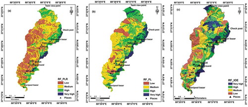
The acquired PLR values are used as input to run the RF model. The landslide susceptibility index values are calculated in the range of 0.001–1.00. Natural jenk classification method is used to classify the resultant map into four classes namely low, medium, high and very high (Pourghasemi et al. 2012; Kaur et al. 2017b, 2018; Thapa et al. 2017b). Finally, the landslide susceptibility map of the RF-PLR model is obtained. Resultant map of LSM shows 3.17%, 18.64%, 39.69% and 38.51% of the total area falls under very high, high, medium and low susceptible zone, respectively (Figure 9(a)). Some parts of Tathangchen Syari and Chandmari wards fall under very high susceptible zones. Daragoan and lower Sichey ward of GMC town falls under low susceptible zone.

Figure 9. Landslide susceptibility map derived from combination of (a) RF-PLR, (b) RF-FL, (c) RF-IOE.

RF-FL model

With the help of the fuzzification process all the factor maps are converted to evidence maps using suitable membership values. All the evidence maps are integrated through RF and the resultant is classified into four classes, i.e. low, medium, high and very high landslide susceptible zones (Figure 9(b)). The output of the landslide susceptibility map of the RF-FL predicts that 10.53%, 34.11%, 42.49% and 12.87% of the total area encompasses under very high, high, medium and low susceptible zone, respectively. Very high susceptible zone occurs within Tathangchen Syari, upper Burtuk, Chandmari, lower and upper MG marg. Even, some patches of very high susceptible zone are observed in Ranipool, Daragoan, development area and Arithang wards of GMC town. Low susceptibility zones area found in upper side of lower Sichey ward-I and upper Sichey, middle of Burtuk and lower Sichey ward-II, Daragoan and Tadong, respectively.

RF-IOE model

The final weight (W_j) of the triggering factors is presented in Table 5. The output of the entropy model shows that factors like distance from road (m), water regime, LULC, aspect, soil thickness, slope are the most important factors having the Wj values of 0.736, 0.557, 0.435, 0.333, 0.225 and 0.129, respectively as these can better explain the landslide occurrences in the study area. The other conditioning factors like elevation (0.090), soil (0.083), curvature (0.074), lineament (0.069), geology (0.013) rainfall (0.0003) show low Wj for the study area. The acquired Wj values are taken as input for RF model. The observed LSI values vary from 0.001 to 1.00. The output of RF-IOE model is classified into four classes low, medium, high and very high using natural jenk classification method (Figure 9(c)) (Pourghasemi et al. 2012; Kaur et al. 2017b, 2018; Chen et al. 2018). The final output of RF-IOE predicts that 16.34%, 32.08%, 30.73% and 20.84% of the total area is under very high, high, medium and low susceptible zone, respectively.

Model performance

Performance of different landslide susceptibility models are evaluated through confusion matrix. Confusion matrix predicts the accuracy of the obtained classification. Accuracy statistics assess the model performance by combining true positive and true negative. RF-PLR model shows type-I error and type-II error of 13% and 23.38%, respectively with overall accuracy of 55.64%, while RF-FL model shows the overall agreement of 69.36% with 9.68% and 19.35% of type-I error and type-II error respectively. RF-IOE model predicts overall agreement 62.89% where the type-I error is 5.6% and type-II is 31.45%. Cohen’s Kappa (Ƙ) index is computed to measures the performance of the statistical classification, which is obtained from confusion matrix (Table 3). The Ƙ value for RF-PLR, RF-FL and RF-IOE is 0.27, 0.70, and 0.35, respectively. The result of Cohen’s Kappa index for RF-PLR and RF-IOE model suggested that the agreement between predicted and observed value is fair. Kappa statistics for RF-FL indicates the substantial agreement of the model. Overall, these above analysis have demonstrated that RF-FL performed very well as compared to other model.

Model comparison

The outputs of the two models applied are compared to each other to measure model compatibility (Brindha and Elango 2015). For the comparison of models, the outputs of both models were reclassified into four classes each namely 1, 2, 3 and 4 representing low, medium, high and very high. The model outputs were subtracted among each other, i.e. RF-PLR-RF-FL, RF-IOE-RF-PLR and RF-IOE-RF-FL to estimate the difference in prediction and the results obtained are represented in Table 6. Zero value indicates the model fitting made by both models is the same with no difference in prediction and value of + and – values represents prediction difference of one zone between two models compared. In all possible combinations the models show the similarity of at least 75%. Comparison of IOE and PLR model shows approximately 79.27% similarity in prediction, about 15% predictions shows difference of 1 susceptibility class higher or lower in prediction and whereas, in the remaining 4% areas, the two models show prediction difference of more than two classes. On comparison of IOE and FL, the models show 86.81% similarity in prediction, about 11% prediction shows a difference of 1 susceptibility class higher or lower. On PLR versus FL comparison, the models show a similarity of about 75.44% and 14% difference in prediction of one susceptibility class higher or lower.

Table 6. Difference in prediction in susceptibility classes between three models.

	Difference in vulnerability classes (%)
Model compared	−3	−2	−1	0	1	2	3
RF-PLR-RF-FL	0.45	3.21	4.21	75.44	9.29	6.33	1.07
RF-IOE-RF-PLR	0.0	0.41	4.48	79.27	11.21	2.21	1.42
RF-IOE-RF-FL	0.0	0.0	2.14	86.81	8.57	1.83	0.65

Wilcoxon-signed rank test has been applied to find out the significant statistical differences among three models pairwise viz., RF-PLR vs. RF-FZ, RF-PLR vs. RF-IOE and RF-FZ vs. RF-IOE. This test deduce, is there any difference between the performances of the models at 5% (α = 0.05) significance level. So, the p value and z value for this test for our models under our data have been calculated.

Bui et al. (2016); Sahin, Ipbuker, and Kavzoglu (2017); Merghadi, Abderrahmane, and Bui (2018) already used Wilcoxon signed-rank test for calculating the statistically significant differences between three different models of landslide susceptibility. From Table 7, concluded that there is a significant difference in the performance result between each pair of models except RF-FL and RF-IOE pair. The obtained p value > 0.05 and the z value did not exceeded the critical values for RF-FZ vs. RF-IOE models.

Table 7. Pair wise comparison of the three landslide susceptibility models using Wilcoxon signed rank test.

Sl no.	No. pair wise comparison	z value	p value	Significance
1	RF-PLR vs. RF-FZ	−2.397^b	0.017	Yes
2	RF-PLR vs. RF-IOE	−2.201^b	0.028	Yes
3	RF-FZ vs. RF-IOE	−0.510^b	0.610	No

Model validation

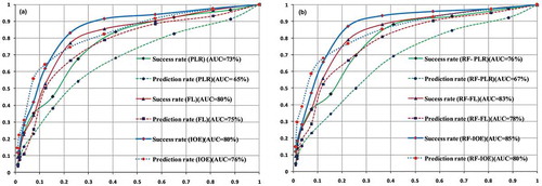
In order to find out the comparative assessment of the techniques used for landslide susceptibility zonation, validation is the necessary step (Begueria 2006). Success and prediction rate (Chung and Fabbri 2003) is a very widely implemented technique for model validation. First of all, the landslide inventory is divided into two datasets, i.e. modelling and validation. Out of the total landslide inventories, 25% data are randomly classified into the validation group (Neuhauser, Damm, and Terhorst 2012; Kaur et al. 2017b; Thapa et al. 2017b; Thapa et al. 2017c). The obtained susceptibility index values are distributed into cumulative interval values of 1% by dividing it into 100 equal classes. To generate the success rate curve (SRC) of the model, the cumulative percentage of predicted landslide susceptible areas on the x axis are plotted against the cumulative percentage of landslide area in the training dataset on the y axis (Chung and Fabbri 2003; Sterlacchini et al. 2011). SRC provides the rate of prediction but does not provide any information about the accuracy of prediction (Thapa, Gupta, and  Kaur 2017d). This is where the prediction rate curve (PRC) comes into play by evaluating the accuracy of future predictions made on the basis of SRC. PRC was obtained by a similar process to SRC but with cumulative percentage of landslide area in the testing dataset on the y axis (Chung and Fabbri 2003). Figure 10 represents the SRC and PRC for single techniques (PLR, FL, IOE) and hybrid technique (RF-PLR, RF-FL, RF-IOE), respectively. In terms of the success rate curve, the success rate of the model is 76%, 83% and 85% for RF-PLR, RF-FL and RF-IOE models, respectively. The success rate of the prediction rate curve is 67%, 78% and 80% for RF-PLR, RF-FL and RF-IOE models, respectively. The success and prediction rate curves show the RF-IOE model gives more accurate results compared to other two hybrid models.

Figure 10. Success and prediction rate curve (a) for PLR, FL and IOE, (b) for RF-PLR, RF-FL, RF-IOE.

Conclusions

The research work represents the application of new hybrid techniques for Landslide susceptibility mapping. On the basis of the final output RF_IOE around 1079 building structure with a population of 5226 and 5833 building structure with a population of 23,103 falls on very high and high zone, respectively (Supplementary Figure 1). Around 4551 building structure falls in medium zone having a population of about 20,655 whereas 935 building structure with a population of 7070 falls on low susceptible zone. In addition, there were 46 building refused the surveys in the study area. These problematic zones are found under Darjeeling gneiss and phyllite, schist zone. The reason behind landslide occurrences in these problematic zones is that there is a sinking zone along Indira Bypass road (west of Gangtok city) and Chandmari area (east of Gangtok city). Landslides near Indira Bypass road are caused due to the formation of vulnerable wedge along the slope and huge stepped chute drains have been constructed. These chute drains require firm foundation for its stability. In general, it has been observed that these chute drains have been founded on loosely compacted slide debris. As a result, most of these chute drains get damaged or failed development of several gapping joints, transverse and longitudinal cracks at several locations. Water leakage has been also observed through these cracks. The foliation joint altitude varies from 45° to 60°. The unguided surface and subsurface drain courses get more energized during rainy season and continued piping action become more vigorous resulting high rate of creep and subsidence in this unstable slope in rainy season. In central part of the Chandmari area a well-marked subsidence zone is present, where the road bench has been subsided in order of 1–1.5 m (maximum). In this zone weathering of weaker rock mica schist bands within harder gneiss rock along with percolation of water through wide gaping joints within the gneissic blocks which acts as lubricator thereby reducing shear strength of the rock. Near Ranipool (South of Gangtok city) high and very high landslide susceptibility zones are observed. This part poses a problem due to (i) the effect of continuous creep and subsidence along the slope because of heavy saturation of unconsolidated and heterogeneous overburden material, (ii) road cutting along Ranipool Pakyong road and (iii) this area is exposed to highly weathered and decomposed schist and phyllite. Based on detailed study a number of remedial measures have been suggested which are as follows: (i) guniting/wire mesh shotcreting of the gneiss rock outcrops with proper water release hole, (ii) repairing the existing surface and subsurface drainage system (chute and contour drains).

Seismic activity influences the stability of the slope as there are many inventory records of landslides triggered by earthquakes. So, there is a need to add seismic data as an input factor layer for regions that are seismically active. Furthermore, decision tree and multivariate techniques can be applied to check the superiority of the geostatistical techniques in study area. This work will help the authority and community to mitigate hazards and prepare for response to and recovery from hazard events.

Acknowledgments

The author would thankful to Department of Science and Technology, India for providing the fund under INSPIRE Fellowship (DST/INSPIRE Fellowship/2015/IF150309) to carry out the research work. The authors are grateful to Sikkim State Disaster Management Authority (SSDMA), India for their help and valuable contributions. The author would also like to thank the Geological Survey of India (GSI), Survey of India (SoI), Indian Meteorological Department (IMD) for their published information, help and support.

Disclosure statement

No potential conflict of interest was reported by the authors.

Supplementary Material

Supplemental data for this article can be accessed here.

Additional information

Funding

This work was supported by the Department of Science and Technology (DST), India [DST/INSPIRE Fellowship/2015/IF150309]; Department of Science and Technology (DST), India [DST/INSPIRE Fellowship/2015/IF150309].

References

- Allouche, O., A. Tsoar, and R. Kadmon. 2006. “Assessing the Accuracy of Species Distribution Models: Prevalence, Kappa and the True Skill Statistic (TSS).” Journal of Applied Ecology 43: 1223–1232. doi:10.1111/j.1365-2664.2006.01214.x.
- Althuwaynee, O. F., B. Pradhan, H. J. Park, and J. H. Lee. 2014. “A Novel Ensemble Decision Tree-Based CHi-squared Automatic Interaction Detection (CHAID) and Multivariate Logistic Regression Models in Landslide Susceptibility Mapping.” Landslides 11: 1063. doi:10.1007/s10346-014-0466-0.
- Althuwaynee, O. F., B. Pradhan, and S. Lee. 2012. “Application of an Evidential Belief Function Model in Landslide Susceptibility Mapping.” Computers & Geosciences 44: 120–135. doi:10.1016/j.cageo.2012.03.003.
- Anbalagan, R., R. Kumar, K. Lakshmanan, S. Parida, and S. Neethu. 2015. “Landslide Hazard Zonation Mapping Using Frequency Ratio and Fuzzy Logic Approach, a Case Study of Lachung Valley, Sikkim.” Geoenvironmental Disasters 2: 6. doi:10.1186/s40677-014-0009-y.
- Basharat, M., H. R. Shah, and N. Hameed. 2016. “Landslide Susceptibility Mapping Using GIS and Weighted Overlay Method: A Case Study from NW Himalayas, Pakistan.” Arabian Journal of Geosciences 9: 292. doi:10.1007/s12517-016-2308-y.
- Begueria, S. 2006. “Validation and Evaluation of Predictive Models in Hazard Assessment and Risk Management.” Natural Hazards 37: 315–329. doi:10.1007/s11069-005-5182-6.
- Bhasin, R., E. Grimstad, J. Larsen, A. K. Dhawan, R. Singh, S. K. Verma, and K. Venkatachalam. 2002. “Landslide Hazards and Mitigation Measures at Gangtok, Sikkim Himalaya.” Engineering Geology 64: 351–368. doi:10.1016/S0013-7952(01)00096-5.
- Brabb, E. E. 1984. “Innovative Approaches to Landslide Hazard Mapping”. In Proceedings 4th International Symposium on Landslides, 1, 307–324. Toronto.
- Breiman, L. 2001. “Random Forests.” Machine Learning 45: 5. doi:10.1023/A:1010933404324.
- Brindha, K., and L. Elango. 2015. “Cross Comparison of Five Popular Groundwater Pollution Vulnerability Index Approaches.” Journal of Hydrology 524: 597–613. doi: 10.1016/j.jhydrol.2015.03.003.
- Bui, D. T., B. T. Pham, Q. H. Nguyen, and N. D. Hoang. 2016. “Spatial Prediction of Rainfall-Induced Shallow Landslides Using Hybrid Integration Approach of Least-Squares Support Vector Machines and Differential Evolution Optimization: A Case Study in Central Vietnam.” International Journal of Digital Earth. doi:10.1080/17538947.2016.1169561.
- Carson, M. A., and M. J. Kirkby. 1972. Hillslope Form and Process, 475. London: Cambridge University Press.
- Chakraborty, I., S. Ghosh, D. Bhattacharya, and A. Bora. 2011. “Earthquake induced landslides in the Sikkim-Darjeeling Himalayas - An aftermath of the 18th September 2011 Sikkim earthquake.” Geological Survey of India, Kolkata. http://www.sikenvis.nic.in/writereaddata/Earthquake%20induced%20landslides%20in%20the%20Sikkim-Darjeeling%20Himalaya.pdf
- Champati Ray, P. K., S. Dimri, R. C. Lakhera, and S. Sati. 2007. “Fuzzy-Based Method for Landslide Hazard Assessment in Active Seismic Zone of Himalaya.” Landslides 4: 101–111. doi:10.1007/s10346-006-0068-6.
- Chawla, A., S. Chawla, S. Pasupuleti, C. S. Rao, K. Sarkar, and R. Dwivedi. 2018. “Landslide Susceptibility Mapping in Darjeeling Himalayas, India.” Hindawi, Advances in Civil Engineering 2018. doi:10.1155/2018/6416492.
- Chen, T., R. Niu, B. Du, and Y. Wang. 2014. “Landslide Spatial Susceptibility Mapping by Using GIS and Remote Sensing Techniques: A Case Study in Zigui County, the Three Georges Reservoir, China.” Environmental Earth Sciences 73 (9): 5571–5583. doi:10.1007/s12665-014-3811-7.
- Chen, W., H. Han, B. Huang, Q. Huang, and X. Fu. 2018. “A Data-Driven Approach for Landslide Susceptibility Mapping: A Case Study of Shennongjia Forestry District, China.” Geomatics, Natural Hazards and Risk 9 (1): 720–736. doi:10.1080/19475705.2018.1472144.
- Chen, W., H. R. Pourghasemi, M. Panahi, A. Kornejady, J. Wang, X. Xie, and S. Cao. 2017a. “Spatial Prediction of Landslide Sus-ceptibility Using an Adaptive Neuro-fuzzy Inference System Combined with Frequency Ratio, Generalized Additive Model, and Support Vector Machine Techniques.” Geomorphology 297: 69–85. doi:10.1016/j.geomorph.2017.09.007.
- Chen, W., W. Li, H. Chai, E. Hou, X. Li, and X. Ding. 2016. “GIS-based Landslide Susceptibility Mapping Using Analytical Hierarchy Process (AHP) and Certainty Factor (CF) Models for the Baozhong Region of Baoji City, China.” Environmental Earth Science 75: 63. doi:10.1007/s12665-015-4795-7.
- Choubey, V. D. 1992. “Landslide Hazards and their Mitigation in the Himalayan Region”.In Proceedings of the Sixth International Symposium on Landslide, 1849–1868. Christchurch, New Zealand, February 10–14.
- Chung, C. J. F., and A. G. Fabbiri. 2001. “Prediction Models for Landslide Hazard Zonation Using a Fuzzy Set Approach.” In Geomorphology and Environmental Impact Assesment, edited by M. Marchetti and V. Rivas, 31–47. Rotterdam: Balkema Publishers.
- Chung, C. J. F., and A. G. Fabbiri. 2005. “Systematic Procedures of Landslide Hazard Mapping for Risk Assessment Using Spatial Prediction Models.” In Landslide Hazard and Risk, edited by T. Glade, M. G. Anderson, and M. J. Crozier, 139–177. New York: Wiley.
- Chung, C. J. F., and A. G. Fabbiri. 2003. “Validation of Spatial Prediction Models for Landslide Hazard Mapping.” Natural Hazards 30 (3): 451–472. doi:10.1023/B:NHAZ.0000007172.62651.2b.
- Ciurleo, M., L. Cascini, and M. Calvello. 2017. “A Comparison of Statistical and Deterministic Methods for Shallow Landslide Susceptibility Zoning in Clayey Soils.” Engineering Geology 223 (7): 71–81. doi:10.1016/j.enggeo.2017.04.023.
- Dai, F. C., and C. F. Lee. 2002. “Landslide Characteristics and Slope Instability Modeling Using GIS, Lantau Island, Hong Kong.” Geomorphology 42 (3): 213–228. doi:10.1016/S0169-555X(01)00087-3.
- Dehnavi, A., I. N. Aghdam, B. Pradhan, and M. H. M. Varzandeh. 2015. “A New Hybrid Model Using Step-wise Weight Assessment Ratio Analysis (SWARA) Technique and Adaptive Neuro-fuzzy Inference System (ANFIS) for Regional Landslide Hazard Assessment in Iran.” CATENA 135: 122–148. doi:10.1016/j.catena.2015.07.020.
- Dietterich, T. G. 2000. “”An Experimental Comparison of Three Methods for Constructing Ensembles of Decision Trees: Bagging, Boosting, and Randomization.” Machine Learning 40: 139–157. doi:10.1023/A:1007607513941.
- Dragicevi, C. S., T. Lai, and S. Balram. 2015. “GIS-based Multicriteria Evaluation with Multiscale Analysis to Characterize Urban Landslide Susceptibility in Data-Scarce Environments.” Habitat International 45: 114–125. doi:10.1016/j.habitatint.2014.06.031.
- Ercanoglu, M., and C. Gokceoglu. 2002. “Assessment of Landslide Susceptibility for a Landslide-Prone Area (North of Yenice, NW Turkey) by Fuzzy Approach.” Environmental Geology 41: 720–730. doi:10.1007/s00254-001-0454-2.
- Frattini, P., G. Crosta, and A. Carrara. 2010. “Techniques for Evaluating the Performance of Landslide Susceptibility Models.” Engineering Geology 111: 62–72. doi:10.1016/j.enggeo.2009.12.004.
- Gentile, F., G. Elia, and R. Elia. 2010. “Analysis of the Stability of Slopes Reinforced by Roots.” WIT Transactions on Ecology and the Environment 138. doi:10.2495/DN100171.
- Gerrard, J. 1994. “The Landslide Hazard in the Himalayas: Geological Control and Human Action.” Geomorphology 10: 221–230. doi:10.1016/0169-555X(94)90018-3.
- Ghosh, S., T. B. Ghoshal, J. Mukherjee, and S. Bhowmik. 2016. “Landslide Compendium on Darjeeling-Sikkim Himalayas, India.” In Geological Survey of India. India: GSI, ISSN0 254-0436.
- Glade, T., and M. J. Crozier 2005. “The Nature of Landslide Hazard Impact.” In Landslide Hazard and Risk, edited by T. Glade, M. G. Anderson, and M. J. Crozier, 43–74. Chichester: Wiley. doi:10.1002/9780470012659.ch2.
- Gupta, S., H. Kaur, S. Parkash, and R. Thapa. 2018. “Landslide Susceptibility Zonation of Gangtok city, Sikkim using Knowledge Driven Method (KDM).” Disaster Advances 11 (11): 34–43.
- Guzzetti, F., A. Carrara, M. Cardinali, and P. Reichenbach. 1999. “Landslide Hazard Evaluation: A Review of Current Techniques and Their Application in a Multi-Scale Study, Central Italy.” Geomorphology 31: 181–216. doi:10.1016/S0169-555X(99)00078-1.
- Guzzetti, F., A. C. Mondini, M. Cardinali, F. Fiorucci, M. Santangelo, and K. T. Chang. 2012. “Landslide Inventory Maps: New Tools for an Old Problem.” Earth Science Review 112: 42–66. doi:10.1016/j.earscirev.2012.02.001.
- Guzzetti, F., M. Cardinali, P. Reichenbach, and A. Carrara. 2000. “Comparing Landslide Maps: A Case Study in the Upper Tiber River Basin, Central Italy.” Environment Management 25 (3): 247–363. doi:10.1007/s002679910020.
- Guzzetti, F., P. Reichenbach, M. Cardinali, M. Galli, and F. Ardizzone. 2005. “Probabilistic Landslide Hazard Assessment at the Basin Scale.” Geomorphology 72: 272–299. doi:10.1016/j.geomorph.2005.06.002.
- Hong, H., J. Liu, D. T. Bui, B. Pradhan, T. D. Acharya, B. T. Pham, A. X. Zhu, W. Chen, and B. B. Ahmad. 2018. “Landslide Susceptibility Mapping Using J48 Decision Tree with AdaBoost, Bagging and Rotation Forest Ensembles in the Guangchang Area (China).” CATENA 163: 399–413. doi:10.1016/j.catena.2018.01.005.
- Hong, Y., R. Adler, and G. Huffman. 2007. “Use of Satellite Remote Sensing Data in the Mapping of Global Landslide Susceptibility.” Natural Hazards 43: 245. doi:10.1007/s11069-006-9104-z.
- India Meteorological Department (IMD). 2007. “Meteorological Data in Respect of Gangtok and Tadong Station.“ Meteorological Center, Gangtok: India Meteorological Department, Ministry of Earth Sciences, Government of India. Accessed May 7 2008.
- Kannan, K., E. Saranathan, and R. Anbazhagan. 2013. “Landslide Vulnerability Mapping Using Frequency Ratio Model: A Geospatial Approach in Bodi-Bodimettu Ghat Section, Theni District, Tamil Nadu, India.” Arabian Journal of Geosciences 6 (8): 2901–2913.
- Kannan, M., E. Saranathan, and R. Anbalagan. 2015. “Comparative Analysis in GIS-based Landslide Hazard Zonation-A Case Study in Bodi–BodimettuGhat Section, Theni District, Tamil Nadu, India.” Arabian Journal of Geoscience 8: 691–699. doi:10.1007/s12517-013-1259-9.
- Kannan, M., E. Saranathan, and R. Anbazhagan. 2012. “Landslide Vulnerability Mapping Using Frequency Ratio Model: A GIS Approach in Bodi – Bodimettu Ghat Section, Theni District, Tamil Nadu, India.” Arabian Journal of Geoscience. doi:10.1007/s12517-012-0587-5.
- Kanungo, D. P., M. K. Arora, S. Sarkar, and R. P. Gupta. 2009. “Landslide Susceptibility Zonation (LSZ) Mapping - A Review.” Journal of South Asian Studies 2 (1): 81–105.
- Kaur, H., S. Gupta, and S. Parkash. 2017a. “Comparative Evaluation of Various Approaches for Landslide Hazard Zoning: A Critical Review in Indian Perspectives.” Spatial Information Research 25: 389–398. doi:10.1007/s41324-017-0105-7.
- Kaur, H., S. Gupta, S. Parkash, and R. Thapa. 2018. “Application of Geospatial Technologies for Multi-Hazard Mapping and Characterization of Associated Risk at Local Scale.” Annals of GIS 24: 33–46. doi:10.1080/19475683.2018.1424739.
- Kaur, H., S. Gupta, S. Parkash, R. Thapa, and R. Mandal. 2017b. “Geospatial Modelling of Flood Susceptibility Pattern in a Subtropical Area of West Bengal, India.” Environmental Earth Science 76: 339. doi:10.1007/s12665-017-6667-9.
- Kavzolu, T., I. Colkesen, and E. K. Sahin. 2019. “Machine Learning Techniques in Landslide Susceptibility Mapping: A Survey and A Case Study.” In Landslides: Theory, Practice and Modelling, edited by S. P. Pradhan, V. Vishal, and T. N. Singh. doi:10.1007/978-3-319-77377-3.
- Kim, J. C., S. Lee, H. S. Jung, and S. Lee. 2018. “Landslide Susceptibility Mapping Using Random Forest and Boosted Tree Models in Pyeong-Chang, Korea.” Geocarto International 33 (9): 1000–1015. doi:10.1080/10106049.2017.1323964.
- Kiran, V. S. S., Y. K. Srivastava, and M. Jagannadha Rao. 2014. “Utilization of Resourcesat LISS IV Data for Infrastructure Updation and Land Use/Land Cover Mapping - A Case Study from Simlipal Block, Bankura District, W. Bengal.” International Journal of Advance Remote Sensing GIS 3 (1): 592–597. http://technical.cloud-journals.com/index.php/IJARSG/article/view/Tech-273.
- Kumar, R., and R. Anbalagan. 2015. “Landslide Susceptibility Zonation in Part of Tehri Reservoir Region Using Frequency Ratio, Fuzzy Logic and GIS.” Journal of Earth System Sciences 124 (2): 431–448. doi:10.1007/s12040-015-0536-2.
- Lee, S., J. C. Kim, H. S. Jung, M. J. Lee, and S. Lee. 2017. “Spatial Prediction of Flood Susceptibility Using Random-Forest and Boosted-Tree Models in Seoul Metropolitan City, Korea.” Geomatics Natural Hazard and Risk 8 (2): 1185–1203. doi:10.1080/19475705.2017.1308971.
- Lee, S., and M. J. Lee. 2006. “Detecting Landslide Location Using KOMPSAT 1 and its Application to Landslide-Susceptibility Mapping at the Gangneung Area, Korea.” Advances in Space Research 38: 2261–2271.
- Lin, C. W., S. H. Liu, S. Y. Lee, and C. C. Liu. 2006. “Impacts of the Chi-Chi Earthquake on Subsequent Rainfall-Induced Landslides 463 in Central Taiwan.” Engineering Geology 86 (2–3): 87–101. doi:10.1016/j.enggeo.2006.02.010.
- Mathew, J., V. K. Jha, and G. S. Rawat. 2007. “Application of Binary Logistic Regression Analysis and Its Validation for Landslide Susceptibility Mapping in Part of Garhwal Himalaya, India.” International Journal of Remote Sensing 28 (10): 2257–2275. doi:10.1080/01431160600928583.
- Merghadi, A., B. Abderrahmane, and D. T. Bui. 2018. “Landslide Susceptibility Assessment at Mila Basin (Algeria): A Comparative Assessment of Prediction Capability of Advanced Machine Learning Methods.” ISPRS International Journal of Geo-Information 7: 268. doi:10.3390/ijgi7070268.
- Meten, M., N. P. Bhandary, and R. Yatabe. 2015. “Effect of Landslide Factor Combinations on the Prediction Accuracy of Landslide Susceptibility Maps in the Blue Nile Gorge of Central Ethiopia.” Geoenvironmental Disasters 2: 9. doi:10.1186/s40677-015-0016-7.
- Mondini, A. C., A. Viero, M. Cavalli, L. Marchi, G. Herrera, and F. Guzzetti. 2014. “Comparison of Event Landslide Inventories: The Pogliaschina Catchment Test Case, Italy.” Natural Hazards Earth System Science 14: 1749–1759. doi:10.5194/nhess-14-1749-2014,2014.
- Neuhauser, B., B. Damm, and B. Terhorst. 2012. “GIS-based Assessment of Landslide Susceptibility on the Base of the Weights-Of-Evidence Model.” Landslides 9: 511–528. doi:10.1007/s10346-011-0305-5.
- Ohlmacher Gregory, C. 1930. The Relationship Between Geology and Landslide Hazards of Atchison, Kansas, and Vicinity. 1930 Constant Avenue, Lawrence, Kansas, 66047, Kansas: Kansas Geological Survey. http://www.kgs.ku.edu/Current/2000/ohlmacher/ohlmacher.pdf
- Olden, J. D., M. J. Kennard, and B. J. Pusey. 2008. “Species Invasions and the Changing Biogeography of Australian Freshwater Fishes.” Global Ecology Biogeography 17: 25–37.
- Pachauri, A. K., and M. Pant. 1992. “Landslide Hazard Mapping Based on Geological Attributes.” Engineering Geology 32: 81–100. doi:10.1016/0013-7952(92)90020-Y.
- Pathak, D. 2016. “Knowledge Based Landslide Susceptibility Mapping in the Himalayas.” Geoenvironmental Disasters 3: 8. doi:10.1186/s40677-016-0042-0.
- Pourghasemi, H. R., H. R. Moradi, S. M. Fatemi Aghda, C. Gokceoglu, and B. Pradhan. 2013. “GIS-based Landslide Susceptibility Mapping with Probabilistic Likelihood Ratio and Spatial Multi-Criteria Evaluation Models (North of Tehran, Iran).” Arabian Journal of Geosciences. doi: 10.1007/s12517-012-0825-x.
- Pourghasemi, H. R., and N. Kerle. 2016. “Random Forests and Evidential Belief Function-Based Landslide Susceptibility Assessment in Western Mazandaran Province, Iran.” Environmental Earth Sciences 75: 185. doi:10.1007/s12665-015-4950-1.
- Pradhan, B., S. Lee, and M. Buchroithner. 2010. “Remote Sensing and GIS-based Landslide Susceptibility Analysis and Its Cross-Validation in Three Test Areas Using a Frequency Ratio Model.” Photogrammetrie Fernerkundung Geoinformation 1 (16): 17–32. doi:10.1127/1432-8364/2010/0037.
- Ramli, M. F., N. Yusof, M. K. Yusoff, H. Juahir, and H. Z. M. Shafri. 2010. “Lineament Mapping and Its Application in Landslide Hazard Assessment: A Review.” Bulletin of Engineering Geology and the Environment 69: 215–233. doi:10.1007/s10064-009-0255-5.
- Rawat, R. K. 2005. “Geotechnical Investigations of Chandmari Landslide Located on Gangtok-Nathula Road, Sikkim Himalaya, India.” Journal of Himalayan Geology 26 (2): 309–322.
- Regmi, A. D., K. C. Devkota, K. Yoshida, B. Pradhan, and H. R. Pourghasemi, T. Kumamoto, and A. Akgun, A. 2013. “Application of Frequency Ratio, Statistical Index, and Weights-of-Evidence Models and their Comparison in Landslide Susceptibility Mapping in Central Nepal Himalaya”. Arabian Journal of Geosciencesdoi:10.1007/s12517-012-0807-z.
- Saha, A. K., R. P. Gupta, I. Sarkar, M. K. Arora, and E. Csa-plovics. 2005. “An Approach for GIS-based Statistical Landslide Susceptibility Zonation With a case Study in the Himalayas.” Landslides 2: 61–69.
- Sahin, E. K., C. Ipbuker, and T. Kavzoglu. 2017. “Investigation of Automatic Feature Weighting Methods (Fisher, Chi-Square and Relief-F) for Landslide Susceptibility Mapping.” Geocarto International 32 (9): 956–977. doi:10.1080/10106049.2016.1170892.
- Samia, J., A. Temme, A. K. Bregt, J. Wallinga, J. Stuiver, F. Guzzetti, F. Ardizzone, and M. Rossi. 2018. “Implementing Landslide Path Dependency in Landslide Susceptibility Modeling.” Landslides 1–16. doi:10.1007/s10346-018-1024-y.
- Sharma, A. K. 2008. “Landslide and Its Mitigation for Disaster Management Using Remote Sensing and GIS Technique-A Case Study of Gangtok Area, East Sikkim.” Thesis (MSc), Gangtok: Sikkim Manipal University of Health, Medical and Technological sciences.
- Sharma, L. P., N. Patel, M. K. Ghose, and P. Debnath. 2012. “Geo-Spatial Technology Based Landslide Vulnerability Assessment and Zonation in Sikkim Himalayas in India.” Journal of Geomatics 6 (2).
- Sharma, L. P., N. Patel, M. K. Ghose, and P. Debnath. 2014. “Application of Frequency Ratio and Likelihood Ratio Model for Geo-Spatial Modelling of Landslide Hazard Vulnerability Assessment and Zonation: A Case Study from the Sikkim Himalayas in India.” Geocarto International 29 (2): 128–146. doi:10.1080/10106049.2012.748830.
- Sikkim State Disaster Management Authority (SSDMA). 2012. “Multihazards risk vulnerability assessment Gangtok, East Sikkim. Land Revenue and Disaster Management Department.” Government of Sikkim, Gangtok. Accessed April 7 2015. http://www.ssdma.nic.in/CMS/GetPdf?MenuContentID=10201.
- Soeters, R., and C. J. van Westen. 1996. “Slope Instability Recognition, Analysis, and Zonation.” In Landslides, Investigation and Mitigation, Special Report No. 247, edited by K.T. Turner and R. L. Schuster, 129–177. Washington, DC: Transportation Research Board National Research Council.
- Sterlacchini, S., C. Ballabio, J. Blahut, M. Masetti, and A. Sorichetta. 2011. “Spatial Agreement of Predicted Patterns in Landslide Susceptibility Maps.” Geomorphology 125 (1): 51–61. doi:10.1016/j.geomorph.2010.09.004.
- Thapa, R., S. Gupta, A. Gupta, D. V. Reddy, and H. Kaur. 2017a. “Use of Geospatial Technology for Delineating Groundwater Potential Zones with an Emphasis on Water-Table Analysis in Dwarka River Basin, Birbhum, India.” Hydrogeol Journal. doi:10.1007/s10040-017-1683-0.
- Thapa, R., S. Gupta, A. Gupta, D. V. Reddy, and H. Kaur. 2017c. “Use of Geospatial Technology for Delineating Groundwater Potential Zones with an Emphasis on Water-table Analysis in Dwarka River Basin, Birbhum, India.” Hydrogeology Journal 26 (3): 899–922. doi:10.1007/s1004.
- Thapa, R., S. Gupta, and H. Kaur. 2017d. “Delineation of Potential Fluoride Contamination Zones in Birbhum, West Bengal, India, Using Remote Sensing and GIS Techniques.” Arabian Journal of Geosciences 10: 527. doi10.1007/s12517-017-3328-y.
- Thapa, R., S. Gupta, H. Kaur, and R. Mandal. 2018. “Assessment of Manganese Contamination in Groundwater Using Frequency Ratio (FR) Modeling and GIS: A Case Study on Burdwan District, West Bengal, India.” Modeling Earth Systems and Environment 4: 161. doi:10.1007/s40808-018-0433-1.
- Thapa, R., S. Gupta, S. Guin, and H. Kaur. 2017b. “Assessment of Groundwater Potential Zones Using Multi-Influencing Factor (MIF) and GIS: A Case Study from Birbhum District, West Bengal.” Applied Water Sciences 7(7): 4117–4131. doi:10.1007/s1320 1-017-0571-z.
- Tien Bui, D., O. Lofman, I. Revhaug, and O. Dick. 2011. “Landslide Susceptibility Analysis in the Hoa Binh Province of Vietnam Using Statistical Index and Logistic Regression.” Natural Hazards 59: 1413–1444. doi: 10.1007/s11069-011-9844-2.
- Truong, X. L., M. Mitamura, Y. Kono, V. Raghavan, G. Yonezawa, X. Q. Truong, T. H. Do, D. T. Bui, and S. Lee. 2018. “Enhancing Prediction Performance of Landslide Susceptibility Model Using Hybrid Machine Learning Approach of Bagging Ensemble and Logistic Model Tree.” Applied Sciences 8: 1046. doi:10.3390/app8071046.
- Tsangaratos, P., and I. Ilia. 2016. “Comparison of a Logistic Regression and Naïve Bayes Classifier in Landslide Susceptibility Assessments: The Influence of Models Complexity and Training Dataset Size.” CATENA 145: 164-179.
- van Westen, C. J., E. Castellanos, and S. L. Kuriakose. 2008. “Spatial Data for Landslide Susceptibility, Hazard, and Vulnerability 492 Assessment: An Overview.” Engineering Geology 102 (3–4): 112–131. doi:10.1016/j.enggeo.2008.03.010.
- van Westen, C. J., N. Rengers, and R. Soeters. 2003. “Use of Geomorphological Information in Indirect Landslide Susceptibility Assessment.” Natural Hazards 30 (3): 399–419. doi:10.1023/B:NHAZ.0000007097.42735.9e.
- Vijith, H., and G. Madhu 2008. “Estimating Potential Landslide Sites of an Upland Sub-Watershed in Western Ghat’s of Kerala (India) through Frequency Ratio and GIS.” Environment Geology 55: 1397–1405. doi:10.1007/s00254-007-1090-2.
- Wang, Q., W. Li, W. Chen, and H. Bai. 2015. “GIS-based Assessment of Landslide Susceptibility Using Certainty Factor and Index of Entropy Models for the Qianyang County of Baoji City, China.” Journal of Earth System Science 124 (7): 1399–1415. doi:10.1007/s12040-015-0624-3.
- Youssef, A. M., H. R. Pourghasemi, Z. S. Pourtaghi, and M. M. Al-Katheeri. 2016. “Landslide Susceptibility Mapping Using Random Forest, Boosted Regression Tree, Classification and Regression Tree, and General Linear Models and Comparison of Their Performance at Wadi Tayyah Basin, Asir Region, Saudi Arabia.” Landslides 13: 839. doi:10.1007/s10346-015-0614-1.
- Yufeng, S., and J. Fengxiang, 2009. “Landslide Stability Analysis Based on Generalized Information Entropy”. 2009 International Conference on Environmental Science and Information Application Technology, 83–85.
- Zadeh, L. A. 1978. “Fuzzy Sets as a Basis for a Theory of Possibility.” Fuzzy Sets and Systems 1 (1): 3–28. doi:10.1016/0165-0114(78)90029-5.
- Zezere, J. L., E. Reis, R. Garcia, S. Oliveira, M. L. Rodrigues, G. Vieira, and A. B. Ferreira. 2004. “Integration of Spatial and Temporal Data for the Definition of Different Landslide Hazard Scenarios in the Area North of Lisbon (Portugal) “.” Natural Hazard Earth System Sciences 4: 133–146. doi:10.5194/nhess-4-133-2004.
- Zhang, J., C. J. van Westen, H. Tanyas, O. Mavrouli, Y. Ge, S. Bajrachary, D. R. Gurung, M. R. Dhital, and N. R. Khanal. 2018. “How Size and Trigger Matter: Analyzing Rainfall- and Earthquake-Triggered Landslide Inventories 2 and Their Causal Relation in the Koshi River Basin, Central Himalaya.” Natural Hazards Earth System Sciences. doi:10.5194/nhess-2018-109.
- Zhang, K., X. Wu, R. Niu, K. Yang, and L. Zhao. 2017. “The Assessment of Landslide Susceptibility Mapping Using Random Forest and Decision Tree Methods in the Three Gorges Reservoir Area, China.” Environment Earth Science 76: 405. doi:10.1007/s12665-017-6731-5.
- Zhu, A. X., R. Wang, J. Qiao, Q. Cheng-Zhi, C. Yongbo, L. Jing, D. Fei, L. Yang, and T. Zhu. 2014. “An Expert Knowledge-Based Approach to Landslide Susceptibility Mapping Using GIS and Fuzzy Logic.” Geomorphology 214: 128–138. doi:10.1016/j.geomorph.2014.02.003.
- Zhu, A. X., Y. Miao, R. Wang, T. Zhu, Y. Deng, J. Liu, L. Yang, C. Z. Qin, and H. Hong. 2018. “A Comparative Study of an Expert Knowledge-Based Model and Two Data-Driven Models for Landslide Susceptibility Mapping.” CATENA 166: 317–327. doi:10.1016/j.catena.2018.04.003.