An interactive platform for the analysis of landscape patterns: a cloud-based parallel approach

ABSTRACT

Understanding spatial and temporal characteristics of landscape patterns is critical in ecology, since human interactions with their natural environment can significantly impact ecological processes. The common approach to detect changes in landscape patterns is to evaluate the spatial and temporal variation of well known, established metrics. Examples of such metrics include the composition of different land-use class types and the spatial heterogeneity of individual patches. However, computing such metrics over large geographic areas and at fine levels of granularity requires significant computing resources. In addition, conventional software often lack a visual component that is essential for the detection of changes in landscape patterns and knowledge discovery. In this paper, we propose a cloud-based framework to facilitate the estimation and visualization of landscape pattern analysis in both space and time, capitalizing on the cloud computing facilities provided by Amazon EC2. We illustrate the merit of our approach on landscape metrics across the USA for the years 1992, 2001, and 2011 at the county level. Leveraging cloud computing technology provides the flexibility, scalability and portability to different study regions and at variable scales.

KEYWORDS:

• Landscape metrics
• spatial pattern analysis
• interactive visualization
• GIS
• cloud computing

Introduction

The ecological impacts of land use and land cover change are profound, and numerous examples in the literature have highlighted environmental impacts of future urban development (Gustafson 1998; Nagendra, Munroe, and Southworth 2004). To better understand human interactions with natural systems, landscape ecology plays an important role to analyse land use change pattern and spatial fragmentation (Turner and Lynn Ruscher 1988; Turner 1989, 1990). The results of such analyses can further guide decision-making in urban planning and natural ecological studies.

Landscape metrics are best conceived as a set of algorithms for deriving neighbourhood-based spatial characteristics of land cover patches,¹ classes, or an entire landscape mosaic (McGarigal and Marks 1994). In landscape ecology, these metrics are applied for quantifying the linkages between spatial patterns and ecological processes (McGarigal 2002). Common pattern metrics include density, diversity and spatial structure. The patch density metric estimates the total number of patches in the landscape divided by the total landscape area. Higher patch density tends to reflect smaller patch sizes and is indicative of a more fragmented pattern. The patch diversity metric measures the relationships between different types of patches, such as the similarities and differences among different classes in terms of patch number, density, and shape.

Despite the fact that methods and metrics for analysing land use change are well developed, calculating and visualizing them over large geographic areas, at high spatial and temporal resolutions, poses significant computational challenges.

Metrics that capture the spatial structure of the landscape are affected by the scale at which the analysis is conducted. At macro scales, for instance, metrics describe the class of patches, such as the degree of fragmentation, patch accessibility, proximity, clustering, etc.. For micro scales, the shape attributes of individual patches are generally reported, such as shape complexity and shape irregularity.

To date, various landscape metrics have been developed to characterize landscape patterns, with applications to different domains. In an effort to evaluate urban sprawl, Tsai (2005) used size, density, distribution and centrality to quantify compactness of urban forms. In a similar vein, Galster et al. (2001) applied eight dimensions of landscape metrics to provide an empirical measurement of urban sprawl (density, continuity, concentration, clustering, centrality, nuclearity, mixed uses, and proximity). Landscape metrics have also been used to measure natural habitat fragmentation (Blaschke, Tiede, and Heurich 2004; McAlpine and Eyre 2002; Hargis, Bissonette, and David 1998).

The calculation of landscape metrics is typically conducted in specialized software, such as FRAGSTATS, APACK/IAN, PatchAnalyst, and ZonalMetrics (Mladenoff and DeZonia 1997; McGarigal et al. 2002; Mladenoff and DeZonia 2004; Rempel, Kaukinen, and Carr 2012; Adamczyk and Tiede 2017). One major weakness of these software is the lack of visualization for the calculated metrics. Metrics are generally linked with spatial units and displayed in commercial GIS software.

Computational challenges

We recognize that there remain important issues that need to be addressed. First, landscape metrics can be calculated either based on raster or vector data formats. Raster data are more widely used due to the simple data structure and efficient calculation, but are generally less accurate (Wade et al. 2003). Second, studies computing landscape metrics at very fine scales can lead to different results (Ji et al. 2006), possibly revealing hidden patterns. Noteworthy is the realization that both Geographic Information Systems (GIS) and remote sensing technologies have come a long way and are flexible at integrating data from different sources, scales and formats. The third challenge lies in the exponential increase of computational intensity when landscape metrics are estimated at fine resolution and over large regions (Irwin and Bockstael 2007). This computational challenge generally limits the analysis of landscape metrics to a local or at most, regional scale. Thus, there is a trade-off between resolution, extent, and calculation time (Masek, Lindsay, and Goward 2000).

Computational complexity can further be exacerbated by the need to estimate changes in landscape patterns in both space and time (Delmelle et al. 2013). Recent development of multi-core high-performance computing techniques and parallel computing has dramatically improved computational efficiency and the derivation of results at very fine scales (Xie et al. 2010; Huang et al. 2013). Essentially, parallel computing is a form of HPC that utilizes multiple CPUs or GPUs to solve large and complex computational problems in a timely manner (Wilkinson and Allen 2005). Parallel computing techniques have been utilized to mitigate the computational burden of large spatial problems in landscape pattern analyses (Hazen and Berry 1997; Kalluri et al. 2000; Tang, Bennett, and Wang 2011; Gong, Tang, and Thill 2012; Porta et al. 2013; Hohl et al. 2016; Santé et al. 2016). For example, Tang, Bennett, and Wang (2011) developed a parallel agent-based model that simulates land use change; while Porta et al. (2013) developed genetic algorithms to create land use plans in Guitiriz, Spain, while parallel computing techniques were applied to mitigate the computational burden due to a large number of land plots. However, in-house parallel computing resources may not be available. In this paper, we rely on cloud computing technology, which provides a relatively low-cost platform for parallelizing the calculation of landscape metrics. Spatial cloud computing technology allows on-demand access to HPC resources from remote locations (Yang et al. 2011; Yue et al. 2013). During the past decade, cloud computing technologies have been utilized by researchers and scholars to manage, process, analyse, and visualize a variety of spatial problems (Wang, Wang, and Zhou 2009; Baranski, Schaeffer, and Redweik 2010; Gong, Yue, and Zhou 2010; Baranski et al. 2011; Wan et al. 2014; Neene and Kabemba 2017; Tang and Feng 2017).

Visualization challenges

Effectively communicating the results of landscape metric studies at fine spatial and space-time scales across a large extent can also be challenging. A variety of studies address the issue of visualizing large amounts of spatial and space-time data (Gong et al. 2013; Delmelle et al. 2014; Desjardins et al. 2018a; Desjardins et al. 2018b; Desjardins et al. 2018a); but the figures are static, which may occlude key patterns. Interactive visual analytics can facilitate the discovery of patterns and mitigate the challenge of communicating large volumes of information (Szewrański et al. 2017). Interactive visualization platforms may allow users to zoom, pan; select and compare layers and attributes in one or more windows; improve analysis with supplemental graphs, plots, and tables; and other supplemental functionality (Andrienko and Andrienko 1999; MacEachren et al. 2004; Chertov et al. 2005; Kulawiak et al. 2010; Schumann and Tominski 2011; Kinkeldey 2014; Andrienko et al. 2016; Schiewe 2018).

Contributions

In the light of these issues and recent improvement in high-performance computing, our paper is motivated by the need to develop a robust, automated approach that can estimate and visualize significant changes of landscape metrics over a large spatial extent. The contribution of this research mainly lies in two areas: First, by developing an interactive visualization system, we facilitate the comparison of various landscape metrics with one another, ultimately supporting researchers to better understand changes in landscape patterns. In the previous research, a large number of landscape metrics have been developed and used, but their relationships have not been explored in an interactive manner. Second, we leverage on cloud computing resources so that landscape metrics can be estimated, both at fine resolution and over large areas. Our paper fits within the spirit of increasing efforts in the field of GIScience to the development of systems that combine robust geocomputational techniques with visualization modules.

The rest of our paper is organized as follows. In Section 2, we introduce the overall design of the cloud-based framework. In Section 3, we illustrate the merits of our approach on a case study of counties in the United States, where we demonstrate the functionality of our system to facilitate the discovery of landscape patterns. In Section 4, we provide concluding remarks and avenues for future research.

Methodology

Cloud computing-based framework

Figure 1 illustrates the overall design of our framework, which is comprised of three functional components: (1) data pre-processing, (2) data analysis, and (3) visual analytics. The first two components leverage the cloud platform to conduct parallel computing and reduce computation time, while the third component visualizes and consume the results produced by the first two components.

Figure 1. Overall landscape analysis framework.

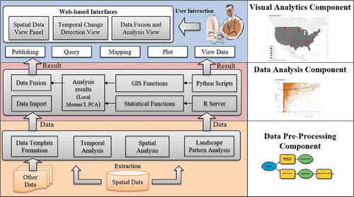
The data pre-processing component organizes a set of GIS workflows, implementing data processing, spatial analysis and landscape metrics calculations. Specifically, the functions include reclassification of land use images and overlay of data layers from different years to detect areas of change.

We calculate several representative landscape metrics for three land cover types, including built-up, natural, and cultivated types (Table 1). These class-level metrics are organized into five groups that represent different landscape characteristics (McGarigal et al. 2002). The first group contains metrics that describe the size and density of patches within a certain area. The second group measures the shape characteristics of the patches. The third group quantifies the proximity of patches, by measuring the nearest distance to neighbouring patches, summarizing the degree of separation. The fourth group concentrates on the contagion and interactions among patches, reflecting the fragmentation pattern. The fifth group evaluates connectivity among patches. We also report the change of these landscape metrics over time.

Table 1. Landscape metrics used in the study.

Category	Metric name
(1) Area/Density	CA (Total (Class) Area)
	NP (Number of Patches)
	PD (Patch Density)
(2) Shape	LSI (Landscape Shape Index)
	PAFRAC (Perimeter-Area Fractal Dimension)
(3)Isolation/Proximity	ENN_MN (Euclidean Nearest Neighbour Distance Mean)
(4) Contagion/Interspersion	CLUMPY (Clumpiness Index)
	PLADJ (Proportion of Like Adjacencies)
	IJI (Interspersion and Juxtaposition Index)
	DIVISION (Landscape Division Index)
	MESH (Effective Mesh Size)
	SPLIT (Splitting Index)
	AI (Aggregation Index)
(5) Connectivity	COHESION (Patch Cohesion Index)

We develop automatic workflows to serialize data processing steps in ArcGIS (ESRI, Redlands, CA) and metrics calculation in FRAGSTATS on Windows-based computers. Using the metric calculation results, further spatial analysis can easily be implemented, such as a correlation or hot spots analysis (local Moran’s I).

The data analysis component implements analytical functions based on the landscape metrics that were derived during the data pre-processing phase. Examples include autocorrelation analysis and hot spot detection, like local Moran’s I (Anselin 1993) from which we can determine the presence of cold and hot spots² revealed in the landscape pattern. Another example is to select a subset of metrics to deal with data redundancy issue (multicollinearity). It is important to note that the data processing and analysis components are implemented in an automatic fashion, while this process can be repeated at different scales and resolution levels.

Due to possible correlation and linear association among different metrics, data redundancy becomes an issue for efficient landscape pattern analysis. Spearman correlation coefficient and variance inflation factor (VIF) criteria measure the presence and magnitude of linear relationships among different metrics (Plexida et al. 2014). Principal component analysis (PCA) and factor analysis (FA) can identify major composite metrics that best explain the variation in the dataset. Several studies suggested to conduct analysis on a smaller set of metrics. For instance, Riitters et al. (1995) applied multivariate factor analysis to reduce 55 calculated metrics to 26 metrics for landscape pattern analysis in the U.S. Plexida et al. (2014) observed higher correlation among metrics at relatively small scale, and subsequently removed 14 highly correlated metrics from the original 24 metrics, using the remaining 10 to investigate the spatial heterogeneity of landscapes in Greece. In this paper, we select out representative metrics to illustrate visualization examples, we quantify the correlation among different landscape metrics. We conduct PCA to identify the first principal component with most explanatory power (Jolliffe 2002).

The visual analytics component provides a visualization portal that gathers data generated from the different analysis processes. We use the Tableau software (Chabot, Stolte, and Hanrahan 2003; Murray 2013) to support interactive data visualization operations. Tableau allows users to organize an interface that can be published as a web portal through the Tableau server, along with interactive visualization functions (data view, zooming, query, ranking, etc.).

Data decomposition and task management

Deriving landscape analysis metrics can be a computationally demanding task, and to complete the analysis in an efficient manner, we rely on computing resources that work in parallel. We apply a cloud computing-based elastic platform (Amazon EC2) to leverage multiple high-performance computing resources according to the problem size. Amazon Elastic Compute Cloud (EC2) is a commercial cloud computing platform that provides virtual computers for rent through a web service. It is elastic because users pay based on the computation time of the resources they use. This computing mode facilitates the centralized management of physical machines and provides efficient computation services without the constraints of geographical location (Amazon 2010).

Two types of tasks are defined for this study. The first task is data decomposition, which divides the entire study area into different spatial units (here, county boundaries). The objective of data decomposition is to follow a divide-and-conquer fashion, in which each computer is in charge of a smaller portion of the overall workload. We consider the calculation of one county as the basic computational block, each with specific calculation intensity (mainly determined by the number of land-use patches). The second type of task implements spatial analysis and landscape calculation for one spatial region (generating raster layers for different land use types using the extracted data of the region). For the second type of task, we follow an embarrassingly parallel approach given no requirement for information exchange among different tasks during the analysis process (Wilkinson and Allen 1999). Therefore, the tasks can be executed independently on different computing nodes.

First, we execute the first type of task to extract land cover data based on user-specified boundaries. Land cover data will then be packaged with the algorithm of calculating landscape metrics for each region, and further be assigned to a computing node. To achieve better workload balance, we use the number of patches within each region to estimate the nodes based on the ecomputational intensity, and maintain a similar amount of work among different computing nodes. Second, we initiate the second type of tasks on their corresponding computing nodes. In the end, we collect the results from the computing nodes for further analysis.

We apply the Windows HPC 2012 Server job manager to orchestra and manage the tasks on the cloud. The scheduling system of Windows HPC includes two major concepts, Job and Task. A job essentially estimates the requirement for computing resources and consists of multiple tasks that define commands, environmental settings, inputs and outputs, and working directories. Users can group jobs based on their running status, check details, modify specific tasks, and edit their execution order. Importantly, jobs can be saved as templates for future modification and replication. We predefine the job template for our metrics calculation task, using the same data input and output folder structures. Therefore, to simply launch a job in the system, we can expect the results to be generated under the same folder.

Application

Data and study area

We demonstrate the usefulness of our approach on a land cover dataset of the United States for the years 1992, 2001, and 2011 (National Land Cover Dataset, a Landsat-based, a 30-m resolution raster dataset). We selected this dataset due to its consistency regarding image classification and fine spatial resolution. County boundaries were obtained from the Census Bureau website (n = 3,109 counties).

Computational results

The estimated sequential computing time for calculating all the landscape metrics reached 575 h (about 24 days). Using 90 CPUs with the load-balancing mechanism, the computing time was significantly reduced to approximately 12 h. Theoretically, if all the subtasks take the same amount of computational time, and each CPU takes the same number of subtasks, the overall computing time can be reduced to about 6 h since the workload is perfectly balanced. And the speedup can be simply improved by adding more computing nodes. However, in a real-world application, it is hardly the case that all the tasks require the exact same amount of computation time. Therefore, load balancing is playing a significant role in adjusting the workload among different computing nodes. It can reduce the idle time for computing nodes and reduce overall processing time.

PCA results

Table 2 reports on the PCA where we identify one metric for each category that captures the most variance in the data (with the highest loading), specifically (1) the number of patches (NP), (2) perimeter-area fractal dimension (PAFRAC), (3) Euclidean nearest neighbour distance mean (ENN_MN), (4) splitting index (SPLIT), and (5) patch cohesion index (COHESION). For the first two groups, the first component (PC1) explains the majority of the data variance (69.6% and 75.2%). For the third category, the three metrics (CLUMPY, PLADJ, and AI) have nearly identical factor loading values, so they can be considered as equally important for representing the variance observed within that group, therefore we can choose either one of them to represent the metric category.

Table 2. Result of principal component analysis.

Category	PC1	PC2	PC3
(1) Area/Density
Standard deviation	1.445	0.955	0.030
Proportion of variance	0.696	0.304	0.000
Factor loadings
CA	0.275	0.962	0.002
NP	0.680	−0.193	0.707
PD	0.680	−0.195	0.707
(2) Shape
Standard deviation	1.227	0.704	–
Proportion of variance	0.752	0.248	–
Factor loadings
LSI	0.707	0.707	–
PAFRAC	0.707	−0.707	–
(3) Structure
Standard deviation	1.734	1.177	1.000
Proportion of variance	0.429	0.198	0.143
Factor loadings
CLUMPY	−0.576	0.001	−0.021
PLADJ	−0.576	0.035	−0.015
IJI	0.015	0.048	−0.861
DIVISION	0.051	0.700	0.002
MESH	−0.037	0.081	0.507
SPLIT	−0.006	−0.707	0.000
AI	−0.576	0.029	−0.019

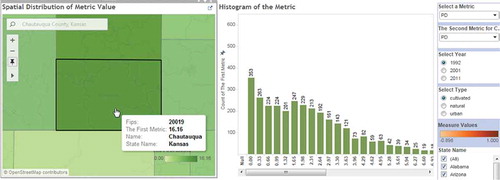
An example of the results from the estimation of changes in landscape metrics is given in Figure 2, using the metric patch density (PD) for urban land cover type for the year 1992. PD values for agriculture land use in 1992 were skewed to the left, suggesting that most counties exhibited small PD values. However, Chautauqua County in Kansas revealed relatively high PD (dark green colour in the map).

Figure 2. Metric calculation example of patch density.

Visualizing distribution and correlation

An overview of the spatial data view panel is given in Figure 3. The panel includes the map canvas, histogram charts, correlation matrix among landscape metrics, and scatterplots. All plots are coordinated with maps and filters; therefore, when different spatial area or data are selected, the plots will change accordingly. The interface provides the selection of year, metrics, and land cover type. Our platform also provides a histogram that summarizes the distribution of values for selected states (in this case, all states are included). The correlation matrix reflects the relationships among different metrics (darker colours in the matrix denote stronger correlation values). In the scatterplot, the two axes correspond to two selected metrics while each dot denotes a specific county. A fitted line shows the general trend of the correlation.

Figure 3. Overview of spatial data view panel.

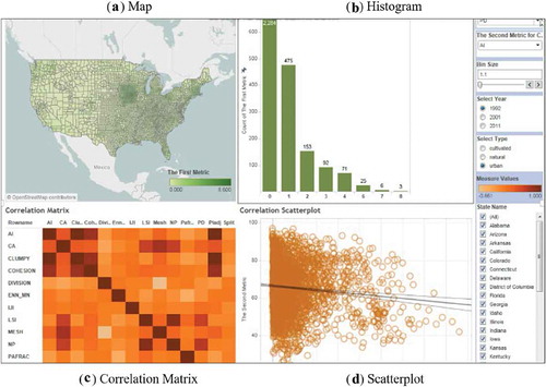
We used the scatterplot of the relationship between PD and AI as an example (Figure 3). The plot reveals that, in our example, a weak negative correlation can be detected between PD and AI for urban land use type among all counties in 1992, with each plot representing metric values for a county. AI measures how much the same class of patches tend to share boundaries; lower AI value denotes that the patches will be less likely to be clustered. Therefore, the correlation here can suggest an early development stage with scattered urban developments. As the leapfrog type of urban development occurs, new urban patches emerge, the landscape is more fragmented by new these scattered developed areas, potentially lead to a lower aggregation level.

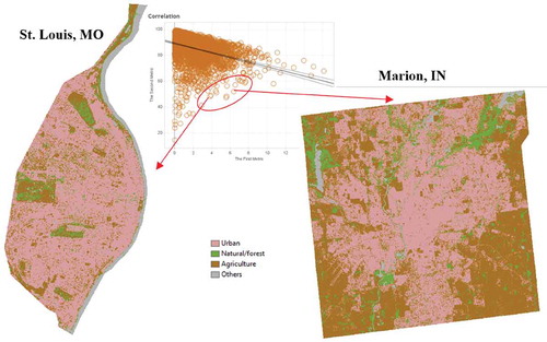
The scatterplot also helps to identify certain types of landscape patterns and detect outliers. In Figure 4 for instance, the points within the red circle fall below the normal level of AI comparing to other points of the same PD value. This can also be interpreted in another way, when the aggregation level is the same with other points, these counties tend to reveal higher patch density than others. St. Louis City (Missouri) and Marion County (Indiana) are both in this case, they exhibit similar low AI and relatively high PD. These regions are both relatively more developed at the time so that the urban patch density is higher than other counties. The low AI could be caused by the on-going urban expansion that pushes the newly urban patches to the county edge.

Figure 4. Identifying region of interest through scatterplot (the first metric is PD and the second metric is AI.

Visualizing change in landscape metrics

Temporal change analysis panels are shown in Figures 5 and 6. Using the longitudinal dataset (years 1992, 2001, 2011), our platform can detect the change of different metrics for a given land cover type. The panel includes a map summarizing the change ratio of specific metrics, while another map illustrates the variation in Local Moran’s I. The two lower plots include a trend line and a bar chart, summarizing the ratio and rank of change, respectively. For instance, using the core area (CA) metric of urban land cover type, the percentage change during these two periods is shown in Figure 5(a,b). The graphs suggest that during the first decade (1992 ~ 2001), several counties were experiencing the drastic change of urban land use patterns, but slower changes during the second decade (2001 ~ 2011) based on the flat pattern of the trend lines in the temporal change chart. Although the increasing pace slowed down in the second period for most of the counties, more cluster patterns have been detected, in which situation more similar changes are detected in neighbouring regions. More specifically, cold spots were detected during the second decade, suggesting a cluster of regions with low metric values.

Figure 5. Temporal change detection panel (an example for metric CA for urban land cover type).

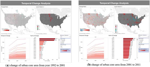
Figure 6. Data fusion panel. The example illustrates the relationship between economic change and urban metrics (CA, AI and Cohesion).

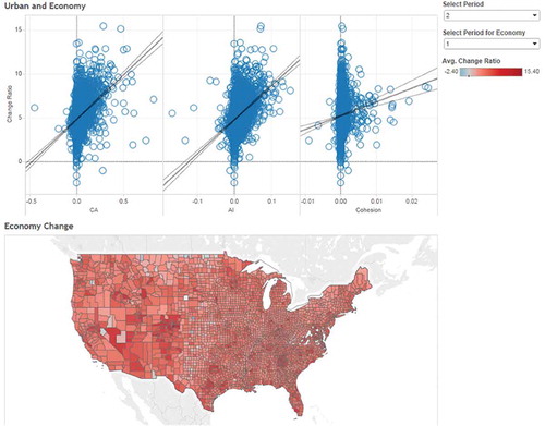
Linking landscape metrics with socio-economic data

The data fusion panel incorporates simple modelling functions to analyse relationships among different datasets. Figure 6 illustrates the relationship between economic growth and urban expansion, between the year of 2001 to 2011. The graph reveals a strong positive relationship between them. In this case study, the economic data are collected from the Bureau of Economic Analysis,³ using the compound annual growth rate for two periods: 1992 to 2001, and 2001 to 2011.

Another example illustrates the changes in landscape metrics and population growth. Growth rate for all the counties is calculated in percentage during year 2000 to 2010, and the change of landscape metrics is calculated for the same two periods. A number of scatterplots summarizing the variation between population growth and land use categories is presented in Figure 7. Interestingly, the scatterplot between CA and population growth shows a positive relationship for urban land use, suggesting that population increase could potentially lead to more demand for land development. The scatterplot between AI and population growth follows a similar pattern.

Figure 7. Data fusion panel (an example of exploring the relationship between population change and landscape metrics).

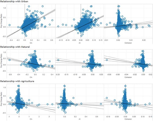
Since our platform facilitates the detection of outliers, once the user selects a set of observations on the plot, the corresponding axis values will then be displayed in a prompt window. Table 3 lists several examples which were visually identified through the scatterplots showing the relationship between urban population change ratio and change in the CA metric. From the scatterplot, most of the observations tend to cluster, and it is relatively straightforward to identify outliers outside of the cluster. These outliers are generally a combination of extremely large or small data values, such as very high population increase rates with high CA, or very low population increases with high CA.

Table 3. Regions of interest based on urban CA metric.

Type of relationship	Population change ratio	Metric change ration	Region
High–high	+110.4%	+53%	Kendall, Illinois
High–low	+109.1%	+12.7%	Pinal, Arizona
Low–high	+8.3%	+74%	Hemphill, Texas
Outlier	−31.5%	−5.9%	Cameron Parish, Louisiana

Discussion and concluding remarks

In this paper, we proposed a platform which combines the computation, analysis, and visualization of landscape metrics to support the detection of changing landscape patterns and ultimately enhancing knowledge discovery. Our platform is robust to estimate landscape metrics over fine resolutions and large extents; and it provides the flexibility for users to select specific spatial units, scales, land cover classifications, and landscape metrics. For example, to study the impact of forest fragmentation on water quality, the users can choose ecologically defined sub-regions or watersheds as the boundaries. For social applications, jurisdictional boundaries can be applied to link with population and economic data to study the correlation between landscape metrics and other economic indicators.

Our system is able to tackle challenges related to metric calculations, including the complexity of spatial data, spatial scale issues, and intensive computation. The application of parallel cloud computing can reduce the computational effort. The elasticity characteristic of cloud computing enables us to recruit more computing resources for demanding spatiotemporal analyses. As such, computing metrics was significantly accelerated, and the application for a large-scale area was conducted within a manageable timeframe. Our system can handle metric calculations under different scales and the automated workflow can be reused to calculate, analyse and publish data whenever users switch to a different scale. Our case study illustrates our approach using a real-world dataset that integrates landscape metrics with social data; it exemplifies the calculation capability for large-scale and high-resolution data. The ability of our approach to identify outliers can serve as a starting point for other studies. Another advantage of our approach is that the calculated results are archived through the Tableau Server, therefore results from landscape metric calculations can be shared with other individuals, promoting knowledge discovery and information exchange.

The process of applying cloud computing is straightforward, in terms of setting up the cluster and arrange the slave-master architecture. We see the following avenues for future research. First, to achieve better computing performance, the importance of load-balancing has been emphasized here. The estimation of computational intensity for individual tasks can guide us to assign jobs to different computing nodes and improve computational efficiency. Similarly to Hohl, Delmelle, and Tang (2015) and Desjardins et al. (2018a), more intelligent decomposition can substantially speed up the process. Second, our approach could incorporate more advanced statistical analyses and data mining functionalities to enhance in-depth knowledge discovery process. For example, further cluster analysis can be developed to group different spatial units that reveal similar landscape pattern changes. Third, we used county boundary as a spatial unit to divide the task – which may not always follow the natural pattern-, and follow an embarrassingly parallel strategy. Since we do not consider the information exchange among different spatial units, we do not deal with edge cases. However, our platform provides the flexibility to conduct spatial analysis based on user-specified boundaries. If the users emphasize the natural boundaries or other types of spatial units, further rules can be defined to deal with data processing involving edges and boundaries. Finally, our platform is loosely coupled in that landscape metrics results are pre-calculated but the analytical process is dynamic and interactive. As future research, a tight integration of cloud-based parallel computing with interactive visualization will allow the user to formulate hypothesis and trigger further computing and interaction with the results.

We hope that our approach can stimulate additional research in other domains, but also lead to further research studying the impact of scale on landscape metrics calculation.

Acknowledgement

The authors would like to acknowledge the feedback and computational support provided by Dr. Wenwu Tang from the Center for Applied Geographic Information Science at the University of North Carolina at Charlotte

Disclosure statement

No potential conflict of interest was reported by the authors.

Notes

1. A patch is the minimum spatial unit for landscape analysis. It has homogeneous characteristics within the area, such as the same land use type.

2.. Cold spots coincide with regions of low values surrounded by areas of low values as well; while hot spots denote high values surrounded by similar high values.

3. https://www.bea.gov/index.htm.

References

- Adamczyk, J., and D. Tiede. 2017. “ZonalMetrics-a Python Toolbox for Zonal Landscape Structure Analysis.” Computers & Geosciences 99: 91–99. doi:10.1016/j.cageo.2016.11.005.
- Amazon, E. C. 2010. “Amazon Elastic Compute Cloud (Amazon Ec2).” Amazon Elastic Compute Cloud (Amazon EC2).
- Andrienko, G., N. Andrienko, J. Dykes, M. J. Kraak, A. Robinson, and H. Schumann. 2016. “GeoVisual Analytics: Interactivity, Dynamics, and Scale.” Cartography and Geographic Information Science 43 (1): 1–2. doi:10.1080/15230406.2016.1095006.
- Andrienko, G. L., and N. V. Andrienko. 1999. “Interactive Maps for Visual Data Exploration.” International Journal of Geographical Information Science 13 (4): 355–374. doi:10.1080/136588199241247.
- Anselin, L. 1993. The Moran Scatterplot as an ESDA Tool to Assess Local Instability in Spatial Association. (pp. 111-125). Morgantown, WV: Regional Research Institute, West Virginia University.
- Baranski, B., T. Foerster, B. Schäffer, and K. Lange. 2011. “Matching INSPIRE Quality of Service Requirements with Hybrid Clouds.” Transactions in GIS 15: 125–142. doi:10.1111/tgis.2011.15.issue-s1.
- Baranski, B., B. Schaeffer, and R. Redweik. 2010. “Geoprocessing in the Clouds.” OSGeo Journal 8 (1): 5.
- Blaschke, T., D. Tiede, and M. Heurich. 2004. “3D Landscape Metrics to Modelling Forest Structure and Diversity Based on Laser Scanning Data.” International Archives of the Photogrammetry, Remote Sensing and Spatial Information Sciences 36 (8/W2): 129–132.
- Chabot, C., C. Stolte, and P. Hanrahan. 2003. Tableau Software.
- Chertov, O., A. Komarov, A. Mikhailov, G. Andrienko, N. Andrienko, and P. Gatalsky. 2005. “Geovisualization of Forest Simulation Modelling Results: A Case Study of Carbon Sequestration and Biodiversity.” Computers and Electronics in Agriculture 49 (1): 175–191. doi:10.1016/j.compag.2005.02.010.
- Delmelle, E., C. Dony, I. Casas, M. Jia, and W. Tang. 2014. “Visualizing the Impact of Space-Time Uncertainties on Dengue Fever Patterns.” International Journal of Geographical Information Science 28 (5): 1107–1127. doi:10.1080/13658816.2013.871285.
- Delmelle, E., C. Kim, N. Xiao, and W. Chen. 2013. “Methods for Space-Time Analysis and Modeling: An Overview.” International Journal of Applied Geospatial Research (IJAGR) 4 (4): 1–18. doi:10.4018/IJAGR.
- Desjardins, M. R., Hohl, A., Griffith, A., & Delmelle, E. (2018a). A space–time parallel framework for fine-scale visualization of pollen levels across the Eastern United States. Cartography and Geographic Information Science, 1-13.
- Desjardins, M. R., A. Whiteman, I. Casas, and E. Delmelle. 2018b. “Space-Time Clusters and Co-Occurrence of Chikungunya and Dengue Fever in Colombia from 2015 to 2016.” Acta Tropica 185: 77–85. doi:10.1016/j.actatropica.2018.04.023.
- Galster, G., R. Hanson, M. R. Ratcliffe, H. Wolman, S. Coleman, and J. Freihage. 2001. “Wrestling Sprawl to the Ground: Defining and Measuring an Elusive Concept.” Housing Policy Debate 12 (4): 681–717. doi:10.1080/10511482.2001.9521426.
- Gong, J., P. Yue, and H. Zhou. 2010. “Geoprocessing in the Microsoft Cloud Computing Platform-Azure.” In Paper presented at the proceedings the joint symposium of ISPRS technical commission IV & autocarto. Orlando, Florida, USA.
- Gong, P., J. Wang, L. Yu, Y. Zhao, Y. Zhao, L. Liang, Z. Niu, et al. 2013. “Finer Resolution Observation and Monitoring of Global Land Cover: First Mapping Results with Landsat TM and ETM+ Data.” International Journal of Remote Sensing 34 (7): 2607–2654. doi:10.1080/01431161.2012.748992.
- Gong, Z., W. Tang, and J.-C. Thill. 2012. “Parallelization of Ensemble Neural Networks for Spatial Land-Use Modeling.” In Paper Presented at the Proceedings of the 5th ACM SIGSPATIAL International Workshop on Location-Based Social Networks. Redondo Beach, CA, USA.
- Gustafson, E. J. 1998. “Quantifying Landscape Spatial Pattern: What Is the State of the Art?” Ecosystems 1 (2): 143–156. doi:10.1007/s100219900011.
- Hargis, C. D., J. A. Bissonette, and J. L. David. 1998. “The Behavior of Landscape Metrics Commonly Used in the Study of Habitat Fragmentation.” Landscape Ecology 13 (3): 167–186. doi:10.1023/A:1007965018633.
- Hazen, B. C., and M. W. Berry. 1997. “The Simulation of Land-Cover Change Using a Distributed Computing Environment.” Simulation Practice and Theory 5 (6): 489–514. doi:10.1016/S0928-4869(96)00026-2.
- Hohl, A., E. M. Delmelle, and W. Tang. 2015. “Spatiotemporal Domain Decomposition for Massive Computation of Space-Time Kernel Density.” ISPRS Annals of Photogrammetry, Remote Sensing & Spatial Information Sciences 2 (4).
- Hohl, A., E. Delmelle, W. Tang, and I. Casas. 2016. “Accelerating the Discovery of Space-Time Patterns of Infectious Diseases Using Parallel Computing.” Spatial and Spatio-Temporal Epidemiology 19: 10–20. doi:10.1016/j.sste.2016.05.002.
- Huang, Q., C. Yang, K. Benedict, S. Chen, A. Rezgui, and J. Xie. 2013. “Utilize Cloud Computing to Support Dust Storm Forecasting.” International Journal of Digital Earth 6 (4): 338–355. doi:10.1080/17538947.2012.749949.
- Irwin, E. G., and N. E. Bockstael. 2007. “The Evolution of Urban Sprawl: Evidence of Spatial Heterogeneity and Increasing Land Fragmentation.” Proceedings of the National Academy of Sciences 104 (52): 20672–20677. doi:10.1073/pnas.0705527105.
- Ji, W., M. Jia, R. W. Twibell, and K. Underhill. 2006. “Characterizing Urban Sprawl Using Multi-Stage Remote Sensing Images and Landscape Metrics.” Computers, Environment and Urban Systems 30 (6): 861–879. doi:10.1016/j.compenvurbsys.2005.09.002.
- Jolliffe, I. 2002. Principal Component Analysis (pp. 1094-1096). Springer Berlin Heidelberg.
- Kalluri, S. N. V., J. Jájá, D. A. Bader, Z. Zhang, J. R. G. Townshend, and H. Fallah-Adl. 2000. “High Performance Computing Algorithms for Land Cover Dynamics Using Remote Sensing Data.” International Journal of Remote Sensing 21 (6–7): 1513–1536. doi:10.1080/014311600210290.
- Kinkeldey, C. 2014. “A Concept for Uncertainty-Aware Analysis of Land Cover Change Using Geovisual Analytics.” ISPRS International Journal of Geo-Information 3 (3): 1122–1138. doi:10.3390/ijgi3031122.
- Kulawiak, M., A. Prospathopoulos, L. Perivoliotis, S. Kioroglou, and A. Stepnowski. 2010. “Interactive Visualization of Marine Pollution Monitoring and Forecasting Data via a Web-Based GIS.” Computers & Geosciences 36 (8): 1069–1080. doi:10.1016/j.cageo.2010.02.008.
- MacEachren, A. M., M. Gahegan, W. Pike, I. Brewer, G. Cai, E. Lengerich, and F. Hardistry. 2004. “Geovisualization for Knowledge Construction and Decision Support.” IEEE Computer Graphics and Applications 24 (1): 13–17.
- Masek, J. G., F. E. Lindsay, and S. N. Goward. 2000. “Dynamics of Urban Growth in the Washington DC Metropolitan Area, 1973-1996, from Landsat Observations.” International Journal of Remote Sensing 21 (18): 3473–3486. doi:10.1080/014311600750037507.
- McAlpine, C. A., and T. J. Eyre. 2002. “Testing Landscape Metrics as Indicators of Habitat Loss and Fragmentation in Continuous Eucalypt Forests (Queensland, Australia).” Landscape Ecology 17 (8): 711–728. doi:10.1023/A:1022902907827.
- McGarigal, K. (2014). Landscape pattern metrics. Wiley StatsRef: Statistics Reference Online.
- McGarigal, K., S. A. Cushman, M. C. Neel, and E. Ene. 2002. FRAGSTATS: Spatial Pattern Analysis Program for Categorical Maps.
- McGarigal, K., and B. J. Marks. 1994. “Spatial Pattern Analysis Program for Quantifying Landscape Structure.” Dolores (CO): PO Box 606: 67.
- Mladenoff, D. J., and B. DeZonia. 1997. APACK 2.0 User’s Guide. Madison, WI, USA: Department of Forest Ecology and Management, University of Wisconsin-Madison.
- Mladenoff, D. J., and B. DeZonia. 2004. “APACK 2.23 Analysis Software: User’s Guide.” Published on Internet server http://www.landscape.forest.wisc.edu/projects/apack
- Murray, D. G. 2013. Tableau Your Data!: Fast and Easy Visual Analysis with Tableau Software. Indianapolis, IN: John Wiley & Sons.
- Nagendra, H., D. K. Munroe, and J. Southworth. 2004. “From Pattern to Process: Landscape Fragmentation and the Analysis of Land Use/Land Cover Change.” Agriculture, Ecosystems & Environment 101 (2): 111–115. doi:10.1016/j.agee.2003.09.003.
- Neene, V., and M. Kabemba. 2017. “Development of a Mobile GIS Property Mapping Application Using Mobile Cloud Computing.” Development 8 (10): 57-68.
- Plexida, S. G., A. I. Sfougaris, I. P. Ispikoudis, and V. P. Papanastasis. 2014. “Selecting Landscape Metrics as Indicators of Spatial heterogeneity—A Comparison among Greek Landscapes.” International Journal of Applied Earth Observation and Geoinformation 26: 26–35. doi:10.1016/j.jag.2013.05.001.
- Porta, J., J. Parapar, R. Doallo, F. F. Rivera, I. Santé, and R. Crecente. 2013. “High Performance Genetic Algorithm for Land Use Planning.” Computers, Environment and Urban Systems 37: 45–58. doi:10.1016/j.compenvurbsys.2012.05.003.
- Rempel, R. S., D. Kaukinen, and A. P. Carr. 2012. “Patch Analyst and Patch Grid.” In Ontario Ministry of Natural Resources. Thunder Bay, Ontario: Centre for Northern Forest Ecosystem Research.
- Riitters, K. H., R. V. O’neill, C. T. Hunsaker, J. D. Wickham, D. H. Yankee, S. P. Timmins, K. B. Jones, and B. L. Jackson. 1995. “A Factor Analysis of Landscape Pattern and Structure Metrics.” Landscape Ecology 10 (1): 23–39. doi:10.1007/BF00158551.
- Santé, I., F. F. Rivera, R. Crecente, M. Boullón, M. Suárez, J. Porta, J. Parapar, and R. Doallo. 2016. “A Simulated Annealing Algorithm for Zoning in Planning Using Parallel Computing.” Computers, Environment and Urban Systems 59: 95–106. doi:10.1016/j.compenvurbsys.2016.05.005.
- Schiewe, J. 2018. “Task-Oriented Visualization Approaches for Landscape and Urban Change Analysis.” ISPRS International Journal of Geo-Information 7 (8): 288. doi:10.3390/ijgi7080288.
- Schumann, H., and C. Tominski. 2011. “Analytical, Visual and Interactive Concepts for Geo-Visual Analytics.” Journal of Visual Languages & Computing 22 (4): 257–267. doi:10.1016/j.jvlc.2011.03.002.
- Szewrański S., Kazak J., Sylla M., Świąder M. 2017. Spatial Data Analysis with the Use of ArcGIS and Tableau Systems. In: Ivan I., Singleton A., Horák J., Inspektor T. (eds) The Rise of Big Spatial Data. Lecture Notes in Geoinformation and Cartography. Springer, Cham.
- Tang, W., D. A. Bennett, and S. Wang. 2011. “A Parallel Agent-Based Model of Land Use Opinions.” Journal of Land Use Science 6 (2–3): 121–135. doi:10.1080/1747423X.2011.558597.
- Tang, W., and W. Feng. 2017. “Parallel Map Projection of Vector-Based Big Spatial Data: Coupling Cloud Computing with Graphics Processing Units.” Computers, Environment and Urban Systems 61: 187–197. doi:10.1016/j.compenvurbsys.2014.01.001.
- Tsai, Y.-H. 2005. “Quantifying Urban Form: Compactness Versus’ Sprawl’.” Urban Studies 42 (1): 141–161. doi:10.1080/0042098042000309748.
- Turner, M. G. 1990. “Spatial and Temporal Analysis of Landscape Patterns.” Landscape Ecology 4 (1): 21–30. doi:10.1007/BF02573948.
- Turner, M. G. 1989. “Landscape Ecology: The Effect of Pattern on Process.” Annual Review of Ecology and Systematics 171–197. doi:10.1146/annurev.es.20.110189.001131.
- Turner, M. G., and C. Lynn Ruscher. 1988. “Changes in Landscape Patterns in Georgia, USA.” Landscape Ecology 1 (4): 241–251. doi:10.1007/BF00157696.
- Wade, T. G., J. D. Wickham, M. S. Nash, A. C. Neale, K. H. Riitters, and K. Bruce Jones. 2003. “A Comparison of Vector and Raster GIS Methods for Calculating Landscape Metrics Used in Environmental Assessments.” Photogrammetric Engineering & Remote Sensing 69 (12): 1399–1405. doi:10.14358/PERS.69.12.1399.
- Wan, J., D. Zhang, Y. Sun, K. Lin, C. Zou, and H. Cai. 2014. “VCMIA: A Novel Architecture for Integrating Vehicular Cyber-Physical Systems and Mobile Cloud Computing.” Mobile Networks and Applications 19 (2): 153–160. doi:10.1007/s11036-014-0499-6.
- Wang Y., Wang S., Zhou D. 2009. Retrieving and Indexing Spatial Data in the Cloud Computing Environment. In: Jaatun M.G., Zhao G., Rong C. (eds) Cloud Computing. CloudCom 2009. Lecture Notes in Computer Science, vol 5931. Springer, Berlin, Heidelberg.
- Wilkinson, B., and C. Allen. 2005. Parallel Programming: Techniques and Applications Using Networked Workstations and Parallel Computers. Upper Saddle River, NJ: Pearson/Prentice Hall.
- Wilkinson, B., and M. Allen. 1999. Parallel Programming. Prentice-Hall, Inc. Upper Saddle River, NJ, USA.
- Xie, J., C. Yang, B. Zhou, and Q. Huang. 2010. “High-Performance Computing for the Simulation of Dust Storms.” Computers, Environment and Urban Systems 34 (4): 278–290. doi:10.1016/j.compenvurbsys.2009.08.002.
- Yang, C., M. Goodchild, Q. Huang, D. Nebert, R. Raskin, X. Yan, M. Bambacus, and D. Fay. 2011. “Spatial Cloud Computing: How Can the Geospatial Sciences Use and Help Shape Cloud Computing?” International Journal of Digital Earth 4 (4): 305–329. doi:10.1080/17538947.2011.587547.
- Yue, P., H. Zhou, J. Gong, and H. Lei. 2013. “Geoprocessing in Cloud Computing Platforms–A Comparative Analysis.” International Journal of Digital Earth 6 (4): 404–425. doi:10.1080/17538947.2012.748847.