Spatio-temporal modelling of wetland ecosystems using Landsat time series: case of the Bajo Sinú Wetlands Complex (BSWC)– Córdoba– Colombia

ABSTRACT

This research is focused on the application of water indexes derived from historical Landsat image series to quantify the impact caused by anthropic activities on wetlands. This work is focused specifically on the Bajo Sinú Wetlands Complex (BSWC) located on the northern Colombian Caribbean Coast. We modelled the spatio-temporal dynamics of the BSWC in three specific periods (1991, 2003 and 2015) and during two seasons: dry and wet. We used data from Landsat 4 Thematic Mapper (TM), Landsat 7 Enhanced Thematic Mapper Plus (ETM) and Landsat 8 Operational Land Imager (OLI) and Thermal Infrared Sensor (TIRS) (Oli-Tirs) images, based on which we evaluated seven different water indexes in order to select the one which best describes changes in the BSWC.

The modelling consisted of the identification of spatio-temporal changes over the BSWC caused by two main pressure factors: (1) anthropic activity in the Sinú River Watershed, which is the main water source of the BSWC and (2) the launch of the Urrá Hydroelectric Dam Project located in the upper basin of the Sinú River in 2000.

The most suitable water index was found to be the Normalized Difference Water Index (NDWI), based on which we acquired water index images and digital classifications. Reliability of these products was rated in terms of the Overall Classification Accuracy values above 87% and a Kappa index between 0.75 and 0.86.

We found that over the 25 year study period, the maximum water storage capacity decreased by 56.2%, the number of the waterbodies reduced by 24.7%, and the average size of the waterbodies decreased by 41%. All the results indicate a deterioration of the water storage capacity in the BSWC.

KEYWORDS:

• Water indexes
• spatio-temporal modelling
• wetlands complex
• permanent water bodies
• Landsat images

Introduction

Importance of wetlands

Wetlands are considered the most valuable landscape elements in the context of providing ecosystem services (Costanza et al. 2014) as they offer habitat to a large number of animal and plant species (Mitsch and Gosselink 2007), improve the quality of water (Sabater et al. 2003; Verhoeven et al. 2006), mitigate damages caused by storms and floods, favour the recovery of aquifers (Gosselink and Turner 1978); (MEA 2005); (Keddy and Fraser 2000); (De Groot et al. 2006), allow for carbon dioxide capture (Hernandez et al. 2015); (Villa and Mitsch 2015); (Estrada et al. 2015), and play a key role in climate change mitigation (Fisher and Turner 2008); (Watanabe and Ortega 2011); (Mitsch et al. 2013).

Despite their importance, wetlands are among the most degraded ecosystems in the world (Finlayson et al. 2013). It was calculated that, in the twentieth century, the world lost between 64% and 71% of its wetlands, a tendency that will likely continue into the twenty-first century (Gardner et al. 2015). Factors that cause the loss of wetland ecosystems include the pressure for land (Soderqvist, Mitsch, and Turner 2000); (Brooks et al. 2005), excessive land exploitation, and the development of projects and activities which cause hydrological changes (Bell 2001), such as the construction of drainage systems, dams and dikes, the deviation of watercourses and underground pumping.

Mapping, inventory, assessment and monitoring of wetlands

According to the Ramsar Convention on Wetlands of International Importance, especially as Waterfowl Habitat (RAMSAR Convention) (Ramsar Convention 2005), the following activities are regarded as key for the wetlands knowledge: mapping, inventory, baseline assessment and wetlands monitoring. According to the Ramsar Convention guidelines, scientists, such as Fluet-Chouinard et al. (2015), ratified the need for an accurate spatial representation of water surfaces and for the identification of types of wetlands, and their extension, and distribution, as a critical activity towards ecological management and decision-making. In addition, the analysis of wetland spatio-temporal dynamics is an important factor in the determination of their degree of decline (Tulbure and Broich 2013).

Despite the recent efforts in the mapping and inventory of wetlands, this data are lacking in many parts of the world. Gardner et al. (2015) suggest that the preparation of public policies aimed at halting the loss of wetlands is limited by the lack of global consensus in terms of delineation of wetlands.

In this regard, technologies for the mapping and monitoring of wetlands are deemed promising (Davidson and Finlayson 2007); (MacKay et al. 2009); (Behera et al. 2012); (Poulin, Davranche, and Lefebvre 2010); (Davranche, Poulin, and Lefebvre 2013). Improvements in the spatial, spectral and temporal resolutions have been significant and a wide range of products, such as Quickbird sensor images, Ikonos and Synthetic Aperture Radar (SAR), is used for the high precision mapping and monitoring of wetlands. There is potential for the combination of SAR, Landsat Thematic Mapper™/Enhanced Thematic Mapper (ETM) and SPOT-5 data in order to improve the accuracy of mapping (MacKay et al. 2009).

The Landsat image gallery, which contains image repositories from 1972 in the form of free access products since 2008, is gaining popularity among the scientific community in the mapping of natural resources at medium scales and documenting historic baselines. Studies that have used these products for the mapping and monitoring of wetlands include Yan et al. (2017) who used optical images, such as Landsat Multispectral Scanner System (MSS), Landsat TM, China Brazil Earth Resources Satellite (CBERS-1) and Landsat Operational Land Imager (OLI), to determine spatial changes in the marshes in the Zhanjiang Plain, China, and calculated the rate of loss of the marsh between 1954 and 2015 from the calculation of landscape indexes. Rokni et al. (2014) used Landsat 5-TM, 7-ETM+ and 8-OLI images to model the spatio-temporal changes in Lake Urmia in Iran, using the water index method. (Li et al. 2013) used the Advanced Land Imager (ALI), TM and ETM + images to compare different water indexes for Land Surface Water (LSW) mapping and found that the ALI data were more accurate and highlights the spatial coverage of the TM and ETM data.

Spectral indexes, among others, have been widely used in the mapping of wetlands (McFeeters 1996); (Xu 2006); (Ji, Zhang, and Wylie 2009). Many studies related to the mapping of waterbodies have utilized these indexes or include a comparison of the effectiveness of the various indexes (Li et al. 2013); (Rokni et al. 2014); (Du et al. 2012); (Mueller et al. 2016); (McFeeters 1996); (Zarco-Tejada, Rueda, and Ustin 2003); (Jackson et al. 2004); (Chipman and Lillesand 2007); (Ouma and Tateishi 2006); (Soti et al. 2009).

Wetlands in Colombia

Colombia has a high bio-geographic, typological and functional diversity, and includes 2,560 ha of wetlands, corresponding to 26.99% of the national territory (Flórez et al. 2016), which are distributed in six regions: Caribbean, Pacific, Mountainous, Orinoquia, Amazonia and Catatumbo (Naranjo 2001). According to Senhadji-Navarro, Ruiz-Ochoa and Rodríguez Miranda (2017), the main impacts affecting these ecosystems include hydrological contamination, changes in hydrological dynamics, desiccation and the spread of invasive species. Patiño (2016) reports that 24.15% of wetlands in Colombia were transformed in 2015 for cattle ranching, and the most affected zones have been the Llanos Piedmont, the Magdalena and Cauca river basins, and the Caribbean Coast.

Bajo Sinú wetlands complex

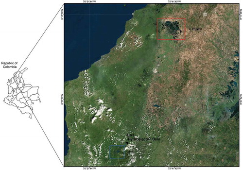
The Bajo Sinú Wetlands Complex (BSWC), is located in northern Colombia at 9°12ʹ19.55ʺ N and 75°45ʹ40.25ʺ W (Figure 1). The BSWC is part of the lower basin of the Sinú River and represents the most low-lying area of a lacustrine-fluvial unit with water and sedimentary contributions from the Sinú River and the Aguas Prietas Stream (IDEAM. Instituto de Hidrología y Meteorología y Estudios Ambientales 1998). It is difficult to calculate its maximum floodplain area because of the continuous changes in its morphological dynamics, associated with the process of land adaptation. This way, the area of maximum flooding for 1998, was estimated at 450 km² (Ramírez González and Viña Vizcaíno 1998), and in 2008 the Autonomous Regional Corporation of the Sinú and San Jorge Valleys (CVS) estimated it in 357 km² (CVS 2008).

Figure 1. Location of BSWC in Córdoba – Colombia.

Ricaurte et al. (2017) found that the main ecosystem services provided by the wetlands in this area include the regulation of water (Campos-Salazar and Gómez Bulla 2011; (Vargas 2015), provision of habitat for species, conservation value, provision of water for human beings, cultural value and the sense of place of local communities. Additionally, the wetlands ensure the quality of life and a source of income for the surrounding communities (Campos-Salazar and Bulla 2011).

The development of the road that connects central Colombia with the coast, the construction of the Urrá Hydroelectric Dam in the upper basin of the Sinú River, the expansion of agriculture and cattle ranching, and urban development (Correa et al. 2006) have negatively impacted ecosystems. For example, the hydrological conditions and sedimentary dynamics have been modified (Vélez Flórez 2009), in turn causing changes in the morphology.

Research context

This research is focused on the evaluation of water indexes based on historic Landsat image series data in order to assess the impact caused by anthropic activities on the BSWC in the northern area of the Colombian Caribbean Coast. This ecosystem has been highly impacted over the last 30 years due to the construction of dykes to provide land for agriculture and cattle ranching activities as well as for the construction of roads and a hydroelectric dam, which is surrounded by a small town with a population of 2,950 people.

We modelled the spatio-temporal dynamics of the BSWC in three specific periods (1991, 2003 and 2015) and two climatic conditions during the year: dry and wet. We used data from Landsat 4 TM, Landsat 7 ETM and Landsat 8 OLI and Thermal Infrared Sensor (TIRS) (Oli-Tirs) images, based on which we evaluated six different water indexes in order to select the one which best describes changes in the BSWC.

This research contributes to the development of indexes for water surface mapping and confirms the results found by Rokni et al. (2014) and Li (2013). In the context of the environmental application, this study presents a specific methodology for the spatio-temporal modelling of wetlands systems using remote sensing techniques based on hydrologic and climatic data. This study contributes to the measurement of the change in water surface area in the BSWC as an indicator of environmental pressure and proposes a methodology for continued monitoring of the BSWC to support decision-making and allow for adaptation to climate change.

Methodology

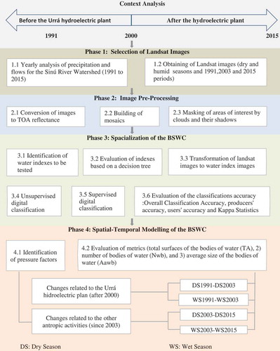
The methodology for this research project can be divided into four phases (Figure 2): (1) the selection of Landsat images, (2) image pre-processing, (3) delimitation of water surfaces and (4) spatio-temporal modelling of the floodplain of the BSWC. These phases will be described in further detail.

Figure 2. Methodological phases.

Selection of Landsat images

The spatio-temporal modelling of the BSWC was related to the seasonal changes in the wetland bodies, taking into account three factors:

1. In tropical areas, seasonal wet and dry periods exhibit differences in the water level. We carried out a yearly analysis of the precipitation and flow for the Sinú River Watershed, the main source of water to the BSWC, over 30 years (1985–2015). From this analysis, we identified wet and dry seasons and these were contrasted using available imagery.

2. The hydrological dynamics of the BSWC were altered in 2000 due to the launch of the Urrá Hydroelectric Dam, located in the upper Sinú River basin.

3. There has been continuous change related to anthropic activity in the Sinú River Watershed and within the BSWC.

From the Landsat TM, ETM, and Oli-Tirs image gallery, available from the United States Geological Service (USGS) Earth Explorer website (USGS 2017), we selected those images that met the aforementioned requirements: four scenes for 1991 (before launch of the Urrá Hydroelectric Dam), four scenes for 2003, following the launch of the Dam, and four scenes for 2015 as a recent reference date. Figure 3 highlights the correlation of selected scenes and seasons, and Table 1 lists the selected scenes.

Table 1. Selected scenes for spatio-temporal modelling of BSWC.

	Scene
Period	10–54	9–54	Season	Sensor
1991	March 14	March 14	Dry	Landsat TM 4
	June 30	June 22	Wet
2003	February 28	February 3	Dry	Landsat 7 ETM +
	June 25	June 2	Wet
2015	February 3	February 12	Dry	Landsat 8 Oli-Tirs
	June 2	June 11	Wet

Figure 3. Selection of Landsat images based on seasonal rainfall conditions.

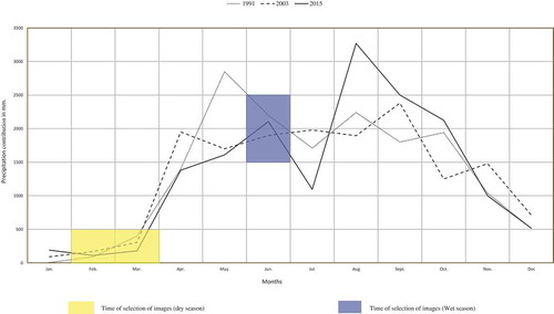
Image pre-processing

Image pre-processing included (1) the conversion of images to Top of Atmosphere (ToA) Reflectance, (2) the building of mosaics which cover the total surface of the BSWC, and the masking of areas of interest covered by clouds and their respective shadows.

Conversion of images to TOA reflectance

For the Landsat 8 Oli-Tirs images, we used equations for calculating the TOA reflectance as suggested by the USGS (as listed on its website):

$\rho \lambda =\left(M_{\rho }{Q}_{\mathrm{C}\mathrm{A}\mathrm{L}}+A_{\rho }\right)/sin\left({\theta }_{\mathrm{S}\mathrm{E}}\right)$

where ρλ is planetary TOA reflectance, M_ρ is the band-specific multiplicative rescaling factor from the metadata, Q_CAL refers to the quantized and calibrated standard product pixel values (DN), A_ρ is the band-specific additive rescaling factor from the metadata, and θ_SE is the local sun elevation angle.

For TM and ETM images, we used the equations suggested by (Chander, Markham, and Helder 2009), who define TOA reflectance with the following equation:

${\rho }_{\lambda }=\pi .L_{\lambda .}{d}^2/ESUN{ }_{\lambda .}cos{\theta }_{\mathrm{s}}$

where

• ρλ = Planetary TOA reflectance (unitless)

• L_λ = spectral radiance (from earlier step)

• d = Earth–Sun distance in astronomical units

• ESUN_λ + = mean solar exoatmospheric irradiances

• θ_s = solar zenith angle

and the calculation of TOA Spectral radiance is based on the following equation:

• L_λ = (LMAX_λ − LMIN_λ/Q_CALMAX − Q_CALMIN(Q_CAL − Q_CALMIN) + LMIN_λ

where

• L_λ = pixel value as radiance

• Q_CAL = digital number

• LMIN_λ = spectral radiance scales to Q_CALMIN

• LMAX_λ = spectral radiance scales to Q_CALMAX

• Q_CALMIN = the minimum quantized calibrated pixel value

• Q_CALMAX = the maximum quantized calibrated pixel value

Building of mosaics

Two Landsat scene frames from path 10 row 54 and path 9 row 54 were used. Despite the high availability of satellite images for this area, it was not possible to select images of the same date for the two path rows. However, each pair of images selected for the building of mosaics was for the same month, and there was a strict control regarding the similarity of weather conditions in the selected images, as shown in Figure 3.

Masking of areas of clouds and their shadows

The problem of sectors intercepted by clouds and cloud shadows was addressed through manual masking of these areas, which generated information gaps in the land-water transition zone. To address this, we used the time series of satellite images available for the closest years and months that contributed data on the presence of water carrying out strict control of precipitation diagrams and total volume of flows.

Delimitation of water surfaces

Selection of water indexes

In order to identify water surfaces across seasons and years, we transformed the satellite images into indexes that highlight land covers of interest, in this case, water. We evaluated several indexes, and selected the one with the best visual differentiation of water cover and applied the decision tree technique, as follows:

1. We used a compilation of water indexes used for several research projects, which can be found in Table 2.

2. Three selected and pre-processed Landsat scenes were selected for this research as follows: (Scene I) TM (path:10 row:54) dated March 1991, (Scene II) ETM (path:10 row:54) dated 25 June 2003, and (Scene III) Oli (path:10 row:54) 1054 dated February 2015. These three scenes included the three product sensors, the three time periods (1991, 2003 and 2015) and the two climatic seasons (dry and wet). The six (6) indexes were calculated for each of these scenes, for a total of 18 index layers.

3. For evaluation of the indexes, three conditions were established: (C1) the best visual definition of the water-land border, (C2) the ability to distinguish small waterbodies and (C3) the best contrast between water and land. Indexes for each scene were evaluated based on the three evaluation conditions as outlined in Figure 4.

4. A grading scale ranging between 1 and 3 was determined for evaluating conditions of each one of the 18 images: (1) does not meet the condition, (2) satisfactory condition and (3) highly satisfactory condition. The first evaluated condition was C1, discarding the images graded with (1) value. This evaluation process was repeated for the two remaining conditions. The index selected was the one where the three Landsat scenes for the images which surpassed the evaluation.

Delimitation of waterbodies for seasonal and annual periods

Once the most suitable water index was selected, the inter-annual and inter-seasonal mosaics were transformed into images of water indexes. From these new images, we carried out supervised classification determining the number of suitable classes at a visual level that would allow for the grouping of pixels in the image without the interference of a ‘Water’ group and an (n−1) ‘No Water’ class. The training phase was adjusted until the error of the assignment of ‘Water’ and other classes using statistical analysis was 0.

Table 2. Water indexes used in different scientific research projects.

Index	Acronym	Equation	Source
Normalized Difference Water Index	NDWI	(Green−NIR)/(Green+NIR)	(McFeeters 1996)
Normalized Difference Water Index de Xu’s or ModifiedNormalizade Difference Water Index	Xu’s NDWI	(Green−MIR)/(Green+MIR)	(Li et al. 2013; Xu 2006)
Normalized Difference Moisture Index	NDMI	(NIR−MIR)/(NIR+MIR)	(Wilson and Sader 2002)
Water Ratio Index	WRI	(Green+Red)/(Green+MIR)	(Shen and Li 2010)
Automated Water Extraction Index	AWEI	4*(Green−MIR)−[(0.25*NIR)+(2.75*SWIR)]	(Feyisa et al. 2014)
Index of Hydrographic Studies Center	I_CEDEX	(NIR/Red)−(NIR/MIR)	(Díaz-Delgado et al. 2006)

The classifications were reclassified for deriving images with two categories: ‘Water’, with a pixel value of 1, and ‘No Water’, with a pixel value of 0. These classifications were evaluated through a confusion matrix, using as reference values of the data of seeds or sampled pixels taken during the training phase, and assigned classes to the pixels as grouped by the classifier (Congalton and Green 2008). We calculated the statistics: Overall Classification Accuracy, producers’ accuracy, users’ accuracy and Kappa Statistics.

Figure 4. Decision tree for index selection.

Reference values were acquired from various sources: for the 2015 period, we used field data taken in periods close to those of the satellite images. For the dry period of 1991, we extracted reference points from aerial photographs, and for the other periods, we used Landsat images closer to the inter-annual and inter-seasonal periods from which we identified control points after an analysis of the spectral signature of each point. The evaluation determined the suitability of assigning a point to one of the two categories: ‘Water’ or ‘No Water’. This coincidence has a higher error probability in the water-land border areas. Therefore, the location of reference points for the evaluation was carried out in these areas.

Mapping of water bodies

For the analysis of the BSWC change dynamics, we considered as a minimum cartographic unit a group of nine pixels (Thompson et al. 2002). Therefore, the groupings with less than nine pixels in the ‘Water’ category were added to the category ‘No Water’. This way, the minimum surface of waterbodies corresponded to 0.81 ha and the scale proposed was 1:100,000.

Modelling dynamics of the floodplain of BSWC

The modelling of the BSWC dynamics was carried out using applied map algebra to the raster layers resulting from the process of classifying the water index mosaics of each of the climatic seasons for the evaluation target years. The results are expressed in hectares, calculated from the pixel size. We considered the two main pressure factors affecting the BSWC: (1) the launch of the Urrá Hydroelectric Dam in 2000, in the upper basin of the Sinú River, which is the main source of water of the BSWC. For the analysis of this factor, we compared the two climatic seasons for the inter-annual periods 1991 (prior to the launch of the Hydroelectric Dam) and 2003 (3 years after the Hydroelectric Dam was launched). (2) The second factor corresponds to anthropic activity in the Sinú River Watershed. For the analysis of this factor, we compared the climatic seasons of the inter-annual periods 2003 and 2015. Specifically, we carried out a raster analysis using three metrics: (1) total surface of the waterbodies (TA), (2) the number of waterbodies (Nwb) and (3) the average area of waterbodies (Aawb). Table 3 shows the map algebra procedure from the raster layers of inter-seasonal and inter-annual mosaics in order to determine the dynamics of the BSWC.

Table 3. Raster operations used for modelling the dynamics of the BSWC. (DS: Dry season, WS: Wet season).

Change Dynamics	Raster operation	Criteria
Permanent water Storage capacity	DS91-DS2003	Influence of the hydroelectric plant
	DS2003-DS2015	Changes overtime (2003–2015)
Maximum capacity of water storage	WS91-WS2003	Influence of the hydroelectric plant
	WS2003-WS2015	Changes overtime (2003–2015)

Results and discussion

Water index for the BSWC cartography

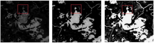
Once the indexes were visually evaluated, we found that the most suitable index was the NDWI, which was found to be true for the three source images. This index shows high contrast for land-water since water shows high reflectance, very low values for areas of dense vegetation, and the water and the borders of other land covers are distinct. Figure 5 shows a section of the contrasted index with an infrared colour composition, which indicates the high differentiation between the three types of covers described.

Figure 5. (a) Infrared colour composition. (b) NDWI Image (Xu 2006).

Although other indexes such as the Modified Normalized Difference Water Index (MNDWI) have good contrast, the potential for visual differentiation of small waterbodies is lower. In Figure 6(a,b) shows images for indexes WRI and NDMI, whereas Figure 6(c) corresponds to the NDWI (Xu 2006), making clear that this last index allows for greater differentiation of waterbodies.

Figure 6. (a) WRI index, (b) NDMI index, and (c) NDWI (Xu 2006).

Although the selection of indexes in this study was carried out employing a qualitative method, we can affirm that this selection is consistent with the results found by Rokni et al. (2014), who compared a group of six indexes to calculate the surface of the Urmia Lake in Iran and found that the indexes that had the lowest absolute error values were the NDWI and NDVI, whereas the NDMI and WRI indexes showed the highest error values.

Likewise, Tulbure et al. (2016) and Li et al. (2013) compared eight different NDWIs, resulting from the combination of green bands and infrared sectors for sensors such as TM, ALI and ETM+. This research found that NDWI (Xu 2006), which combined the green bands and the Shortwave-Infrared (SWIR) of the ALI sensor, was the best index in terms of the detection of water with coefficient values of variation greater than 0.713 and a Kappa coefficient value of 0.9235. However, Gilmore, Saleem and Dewan (2015) found that the MNDWI was the best index for wetlands mapping, whereas the NDWI showed the least appropriate results.

Accuracy assessments of digital classifications

The inter-annual and inter-seasonal mosaics were transformed in water index images based on the NDWI (Xu 2006). For each of the images, we carried out a digital classification. Acquisition of reference information to evaluate the accuracy of cartographic products was complex since information pertaining to specific periods was required. Therefore, it was necessary to search in different sources, as can be demonstrated in Table 4. Ultimately, we derived six contingency matrixes which belong to each of the classifications associated with an inter-annual and inter-seasonal period. Table 4 shows the statistical results used for evaluation of the accuracy. The general accuracy for all the classifications surpasses 85%, whereas the Kappa index ranges between 0.75 and 0.87, which shows that these classifications surpass random classifications by 75%. It is also important to highlight that in order to ensure reliability; the points of reference were located near the borders of waterbodies.

Table 4. Results of the accuracy assessments of digital classifications.

XUS INDEX	Source of verification	Total number of points	No water	Water	Producers’ Accuracy (%)	Users’ Accuracy (%)	Overall Classification Accuracy (%)	Overall Kappa
14 March 1991	Landsat – spectral signatures	150	67	71	89.87	94.67	92.00	0.84
10 June 1991	Aero-photography	150	71	69	94.52	92.00	93.33	0.87
28 February 2003	Landsat – spectral signatures	150	67	65	89.04	86.67	88.00	0.76
25 June 2003	Landsat – spectral signatures	150	71	65	94.20	86.67	90.67	0.81--
3 February 2015	Field data	120	54	51	89.47	85.00	87.50	0.75
2 June 2015	Field data	120	58	48	96.00	80.00	88.33	0.77

Modelling dynamics of the floodplain of BSWC

Table 5 shows the metrics associated with the BSWC. The maximum size of waterbodies was observed in 1991; the minimum in the dry season with 7.269 ha and the maximum in wet seasons with 20.135 ha. The sizes of waterbodies are more homogenous in dry seasons, in which the variation coefficient never surpasses 4, whereas this coefficient reaches 10 during the wet seasons. The correlation coefficient between the number of bodies of water and their size is −0.7.

Table 5. Metrics associated with BSWC for inter-seasonal and inter-annual periods.

	Dry Season			Wet Season
Year	(TA) Total surfacewaterbodies (hectares)	(Nwb) Numberwaterbodies	(Aawb)Averagesize (hectares)	(TA) Total surfacewaterbodies (hectares)	(Nwb) Numberwaterbodies	(Aawb)Averagesize (hectares)
1991	7269	749	9.71	20,135	429	46.90
2003	7930	884	9.00	13,500	719	18.77
2015	6428	699	9.20	8,826	323	27.32

Changes associated with the launch of Urrá Hydroelectric dam

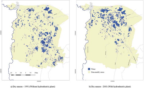
Between 1991 (prior to the launch of the Hydroelectric Dam) and 2003 (3 years after the launch of the Hydroelectric Dam), the surface of permanent waters increased by 9% and the number of waterbodies increased by 18%, but their average sizes decreased by 7.3%. To the left (a) of Figure 7, the location of permanent waterbodies (dry season) for 1991 is shown, and to the right (b) the location of permanent waterbodies for 2003 is shown.

Figure 7. (a) Location of permanent waterbodies (dry season) in 1991 and (b) location of permanent waterbodies in 2003.

Figure 8 illustrates the situation for the wet season in the two periods of time: the dark blue surfaces correspond to the maximum level of water in the wet season for the 1991 and 2003 periods, whereas the brown surfaces represent the maximum levels of water for 1991, and the light blue surfaces, for 2003.

Figure 8. Spatiotemporal dynamics of the BSWC for wet season in 1991 and 2003.

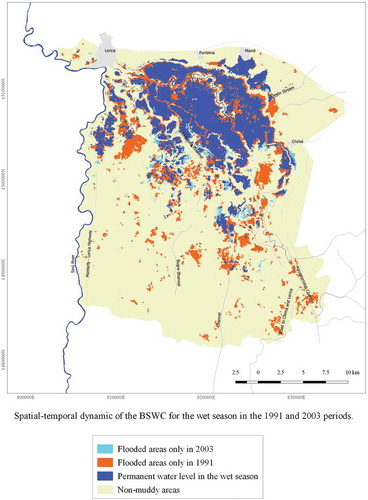
The analysis of the wet seasons for these two periods shows a decrease in the maximum surface capacity (32.9%) and a 67% increase in the number of waterbodies. In other words, there was fragmentation of the BSWC, which shows that, in comparison with 1991, there was a reduction in the volume of water that entered the BSWC in 2003.

The change in extension and the fragmentation of the waterbodies in the BSWC between 1991 and 2003 provides quantitative evidence of the research results of Vélez Flórez (2009), who found that the operation of the Urrá Hydroelectric Dam increased the water flows of the Sinú River in the low water level period (December–April), and decreased the flows in the winter season (May–November). This situation has also been qualitatively described by (Madera Arteaga 2016), based on evidence that the local residents decreased their reliance on agriculture, an activity that they carried out in the riverbeds of wetlands in dry seasons.

The dynamics of change and its resulting impacts on the BSWC is similar to other Colombian wetland complexes where hydroelectric dams have been built without first modelling the impacts, as described by (Angarita et al. 2018). His research determined that such power generating projects built on the Magdalena River have caused the fragmentation of fish spawning routes and a decrease of sediment load in the Mompox Depression (Colombia), and this finding was confirmed in the impact modelling for future hydroelectric projects in this river basin.

Changes in BSWC associated with other anthropic activities in Sinú River Watershed

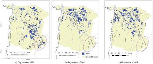
There are permanent changes related to anthropic activities other than the hydroelectric dam in the BSWC. Figure 9(a–c) shows the dry seasons in the three periods of time (1991, 2003 and 2015). From this, it is evident that the permanent waterbodies located on the southeast of the BSWC in the 1991 image disappeared by 2003. The disappearance of these waterbodies is associated with the building of the ‘Las Palomas’ Dam connecting the municipalities of Chimá and Lorica in 1994.

Figure 9. (a–c) Disappearance of permanent waterbodies in BSWC between 1991, 2003 and 2015.

The comparison between the 2003 and 2015 periods shows that the surfaces of permanent water (dry reason) decreased by 19% with a resultant decrease in the number of waterbodies by 20.92% and in their average size by 2%. If we take into account that the average precipitation up-river from the BSWC was constant for the 2 years that were compared (see Figure 10), and the water flow contributed by the Urrá Hydroelectric Dam was 29% higher for February 2015 than for February 2003, we can assume that there was a deterioration of the BSWC in regard to its capacity to cushion and regulate the flows of the Sinú River Watershed. These numbers also confirm the finding of Vargas and Sepulveda (2015) that desiccation of wetlands in this ecosystem is caused by agricultural and cattle ranching activities in the Bajo Sinú (Flórez and Andrés 2009) found that the launching of the Urrá Hydroelectric Dam resulted in a series of drastic changes in the dynamics of both the Sinú River and the areas located downstream of the Dam, which lead to further desiccation of the wetlands.

Figure 10. Spatio-temporal dynamics of BSWC for wet season in 2003 and 2015 periods.

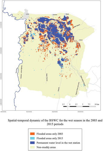
The situation in the wet season is similar: the surface of maximum water capacity for 2015 is 34.6% lower than in 2003. Figure 10 shows that some areas that flooded in the wet season of 2003 did not flood in the wet season of 2015 (highlighted in brown). The areas that remained dry in 2003 but flooded in 2015 are indicated in light blue.

If we take into account that precipitation in the wet seasons of 2003 and 2015 was very similar and the flow released by the Hydroelectric Dam in 2015 was only 8% lower compared to 2003, we can conclude that there was a decrease in the capacity of the BSWC associated with the desiccation of the wetland.

The significant decrease in the number of bodies in wet seasons for the period 2003–2015 and the increase in their average surface area is related to the overall decrease in the water surface of the BSWC, resulting from the construction of dams and an increase in the area dedicated to cattle ranching, as mentioned by Vargas and Sepulveda (2015).

The analysis of the three time periods, both for dry and for wet seasons, shows a tendency for reduction of the total surface for permanent water storage capacity and the storage capacity of maximum levels in the wet season, except during the dry season in 2003. This points to a deterioration of the BSWC in terms of its storage capacity, which is most evident in the wet seasons, where we find an overall decrease of 56% in the water surface area. These results align with the study of the Corporación Autónoma Regional de los Valles del Sinú y del San Jorge; CVS (2008), which explains that the waterlogged area of the BSWC has decreased from 71% of the total area in 1975, to 56% in 1997 and 25.26% in 2008. This trend is evident worldwide, especially in a study of the ecosystems associated with the low Yangtze river basin based on Landsat image series, which showed transformation and development of wetlands (Pal and Saha 2018).

Conclusions

The results of this research, in addition to those reported by Corporación Autónoma Regional de los Valles del Sinú y del San Jorge; CVS (2008) and Ambiotec Ltda (1998) suggest that the tendency towards reduction of the BSWC began before the launch of the Urrá Hydroelectric Dam, resulting from changes in land use. Dixon et al. (2016) proposed a global Wetland Extent Trends (WET) index which found that the extent of wetlands (with the exception of artificial wetlands) decreased by about 30% between 1970 and 2008.

Although we cannot ignore the hydrological and ecological impacts on the BSWC caused by Urrá, it is necessary to understand that the recovery and conservation of these wetland ecosystems are directly associated with limiting agricultural and cattle ranching activities. The cattle ranching activity takes place in the Caribbean Coast Region, especially on the floodplains of the Magdalena River lower basin, and the Cesar, Sucre, Córdoba and Bolívar savannahs (Bustamante Zamudio and Rojas-Salazar n.d.)

This research used a time series of Landsat images to derive indexes that allowed for the delimitation of waterbodies and comparison of these waterbodies over different seasonal and inter-annual periods. It is important to underscore the value of the Landsat repository of images, which supports the sustainable management of resources and scientific research worldwide (Wulder et al. 2016). Without this data, it would have been impossible to reconstruct the processes of change over the three decades. These repositories, as well as the techniques of digital processing in the field of climate change, are essential for building a historical baseline for the quantification of change and loss of hydrological resources and related wetland ecosystems.

There are numerous studies relating to the dynamics of waterbodies based on the calculation of water indexes over a time series, such as Tulbure et al. (2016); Jin et al. (2017); Li et al. (2013); Ariza et al. (2014); Tulbure and Broich (2013); Chen et al. (2014); Díaz-Delgado et al. (2006); Feyisa et al. (2014). However, with regard to the BSWC, this study is the first of its kind.

Various socio-ethnographic and hydrological studies have discussed changes in the hydrodynamics of the Sinú River (the main source of the BSWC) as a result of the operation of the Urrá Hydroelectric Dam that began in 2000. However, there are no previous studies quantifying this impact in the BSWC. This research fills this void.

Furthermore, this study addresses the need identified by Flórez and Andrés (2009) for the quantification of the spatio-temporal alteration of water flow regimes related to Urrá.

We suggest further studies on the dynamics of change in coverage and land use, using the same Landsat time series. It is important to support the findings of this study with data on the anthropic and climate change dynamics in the BSWC over the last 20 years in order to better plan management and conservation strategies.

This study should be duplicated for the series of wetland complexes located downriver from Urrá, including the mangrove ecosystem located on the Sinú River´s estuary.

In terms of the limitations of this study, it is important to mention the resolution of Landsat products, since it was necessary to discard bodies of water less than 0.8 ha at the proposed scale. In these cases, it is necessary to address the results as instruments with explanatory capacity that need to be analysed in light of the socio-environmental contexts.

Acknowledgments

We thank the University of Córdoba for its support in terms of time and logistical resources for this study.

Disclosure statement

No potential conflict of interest was reported by the authors.

Additional information

Funding

This work was supported by the Universidad of Córdoba: [Grant Number FI-03-15

References

- Ambiotec Ltda. 1998. Diagnóstico Ambiental De Las Ciénagas De Lorica Y Betanci. 65. Informe Final: Diagnóstico Ambiental De Las Ciénagas De Lorica Y Betanci.
- Angarita, H., A. J. Wickel, J. Sieber, J. Chavarro, J. A. Maldonado-Ocampo, G. A. Herrera-R, J. Delgado, and D. Purkey. 2018. “Basin-Scale Impacts of Hydropower Development on the Mompós Depression Wetlands, Colombia.” Hydrology and Earth System Sciences 22 (5): 2839. doi:10.5194/hess-22-2839-2018.
- Ariza, A., S. Garcia, S. Rojas, and R. Mauricio. 2014. “Desarrollo De Un Modelo De Corrección De Imágenes De Satélite Para Inundaciones:(CAIN-Corrección Atmosférica E Índices De Inundación).” https://www.researchgate.net/profile/Alexander_Ariza2/publication/313346186_Desarrollo_de_un_modelo_de_correccion_de_imagenes_de_satelite_para_inundaciones_CAIN_-_Correccion_Atmosferica_e_Indices_de_Inundacion/links/58968755aca2721f0dabc772/Desarrollo-de-un-modelo-de-correccion-de-imagenes-de-satelite-para-inundaciones-CAIN-Correccion-Atmosferica-e-Indices-de-Inundacion.pdf
- Arteaga, M., and E. Luis. 2016. Deshaciendo El Encanto: Impactos De La Represa De Urrá I Sobre Tres Comunidades De La Ciénaga Grande De Lorica. Tesis de maestría, Universidad de los Andes, Bogotá, Colombia. http://biblioteca.uniandes.edu.co/acepto1201420.php?id=4698.pdf
- Behera, M. D., V. S. Chitale, A. Shaw, P. S. Roy, and M. S. R. Murthy. 2012. “Wetland Monitoring, Serving as an Index of Land Use Change-A Study in Samaspur Wetlands, Uttar Pradesh, India.” Journal of the Indian Society of Remote Sensing 40 (2): 287–297. doi:10.1007/s12524-011-0139-6.
- Bell, S. S. 2001. “ZEDLER, JB 2000. Handbook for Restoring Tidal Wetlands. CRC Press. 439 P. $89.95. ISBN 0‐8493‐9063‐X.” Limnology and Oceanography 46 (6): 1583. doi:10.4319/lo.2001.46.6.1583.
- Brooks, R. P., D. H. Wardrop, C. A. Cole, and D. A. Campbell. 2005. “Are We Purveyors of Wetland Homogeneity? A Model of Degradation and Restoration to Improve Wetland Mitigation Performance.” Ecological Engineering 24 (4 SPEC. ISS.): 331–340. doi:10.1016/j.ecoleng.2004.07.009.
- Bustamante Zamudio, C., and L. Rojas-Salazar. 2018 “Reflexiones Sobre Transiciones Ganaderas Bovinas En Colombia, Desafíos Y Oportunidades”.. Biodiversidad en la Práctica 3 (1). http://repository.humboldt.org.co/handle/20.500.11761/34599
- Campos-Salazar, L. R., and J. G. Bulla. 2011. “Mariposas (Lepidoptera: Hesperioidea-Papilionoidea) De Las Áreas Circundantes a Las Ciénagas Del Departamento De Córdoba, Colombia.” Revista De La Academia Colombiana De Ciencias Exactas, Físicas Y Naturales 35 (134): 45–60.
- Chander, G., B. L. Markham, and D. L. Helder. 2009. “Summary of Current Radiometric Calibration Coefficients for Landsat MSS, TM, ETM+, and EO-1 ALI Sensors.” Remote Sensing of Environment 113 (5): 893–903. doi:10.1016/j.rse.2009.01.007.
- Chen, L., Z. Jin, R. Michishita, J. Cai, T. Yue, B. Chen, and X. Bing. 2014. “Dynamic Monitoring of Wetland Cover Changes Using Time-Series Remote Sensing Imagery.” Ecological Informatics 24: 17–26. doi:10.1016/j.ecoinf.2014.06.007.
- Chipman, J. W., and T. M. Lillesand. 2007. “Satellite‐Based Assessment of the Dynamics of New Lakes in Southern Egypt.” International Journal of Remote Sensing 28 (19): 4365–4379. doi:10.1080/01431160701241787.
- Congalton, R. G., and K. Green. 2008. Assessing the Accuracy of Remotely Sensed Data: Principles and Practices. CRC press. https://scholar.google.es/scholar?hl=es&as_sdt=0%2C5&q=Assessing+the+Accuracy+of+Remotely+Sensed+Data%3A+Principles+and+Practices&btnG=.
- Corporación Autónoma Regional de los Valles del Sinú y del San Jorge; CVS. 2008. “Plan De Manejo Y Ordenamiento Ambiental Del Complejo Cenagoso Del Bajo Sinú.” Medellin. http://documentacion.ideam.gov.co/cgi-bin/koha/opac-detail.pl?biblionumber=13032&shelfbrowse_itemnumber=13763
- Correa, P., J. Vélez, R. Smith, A. Velez, A. Barrientos, and G. Jesús. 2006. “Metodología De Balance Hídrico Y De Sedimentos Como Herramienta De Apoyo Para La Gestión Integral Del Complejo Lagunar Del Bajo Sinú.” Avances En Recursos Hidráulicos 14 (iii): 71–86.
- Costanza, R., R. de Groot, P. Sutton, S. Van der Ploeg, S. J. Anderson, I. Kubiszewski, S. Farber, and R. Kerry Turner. 2014. “Changes in the Global Value of Ecosystem Services.” Global Environmental Change 26: 152–158. doi:10.1016/j.gloenvcha.2014.04.002.
- Davidson, N. C., and C. M. Finlayson. 2007. “Earth Observation for Wetland Inventory, Assessment and Monitoring.” Aquatic Conservation: Marine and Freshwater Ecosystems 17 (3): 219–228. doi:10.1002/(ISSN)1099-0755.
- Davranche, A., B. Poulin, and G. Lefebvre. 2013. “Mapping Flooding Regimes in Camargue Wetlands Using Seasonal Multispectral Data.” Remote Sensing of Environment 138: 165–171. doi:10.1016/j.rse.2013.07.015.
- De Groot, R., M. Stuip, M. Finlayson, and N. Davidson. 2006. Valuing Wetlands: Guidance for Valuing the Benefits Derived from Wetland Ecosystem Services. Ramsar Technical Report No 3, CBD Technical Series No 27. https://www.cbd.int/doc/publications/cbd-ts-27.pdf.
- Díaz-Delgado, R., J. Bustamante, D. Aragonés, and F. Pacios. 2006. Determining Water Body Characteristics of Doñana Shallow Marshes through Remote Sensing, 3662–3664. http://citeseerx.ist.psu.edu/viewdoc/download?doi=10.1.1.703.3899&rep=rep1&type=pdf
- Dixon, M. J. R., J. Loh, N. C. Davidson, C. Beltrame, R. Freeman, and M. Walpole. 2016. “Tracking Global Change in Ecosystem Area: The Wetland Extent Trends Index.” Biological Conservation 193: 27–35. doi:10.1016/j.biocon.2015.10.023.
- Du, Z., L. Bin, F. Ling, L. Wenbo, W. Tian, H. Wang, Y. Gui, B. Sun, and X. Zhang. 2012. “Estimating Surface Water Area Changes Using Time-Series Landsat Data in the Qingjiang River Basin, China.” Journal of Applied Remote Sensing 6 (1): 063609. doi:10.1117/1.JRS.6.063609.
- Estrada, G., C. Duque, M. L. Gomes Soares, V. Fernadez, and P. M. M. de Almeida. 2015. “The Economic Evaluation of Carbon Storage and Sequestration as Ecosystem Services of Mangroves: A Case Study from Southeastern Brazil.” International Journal of Biodiversity Science, Ecosystem Services & Management 11 (1): 29–35. doi:10.1080/21513732.2014.963676.
- Feyisa, G. L., H. Meilby, R. Fensholt, and S. R. Proud. 2014. “Automated Water Extraction Index: A New Technique for Surface Water Mapping Using Landsat Imagery.” Remote Sensing of Environment 140: 23–35. doi:10.1016/j.rse.2013.08.029.
- Finlayson, C. M., J. A. Davis, P. A. Gell, R. T. Kingsford, and K. A. Parton. 2013. “The Status of Wetlands and the Predicted Effects of Global Climate Change: The Situation in Australia.” Aquatic Sciences 75 (1): 73–93. doi:10.1007/s00027-011-0232-5.
- Fisher, B., and R. Kerry Turner. 2008. “Ecosystem Services: Classification for Valuation.” Biological Conservation 141 (5): 1167–1169. doi:10.1016/j.biocon.2008.02.019.
- Flórez, C., L. M. Estupiñán-Suárez, S. Rojas, C. Aponte, M. Quiñones, Ó. Acevedo, S. Vilardy, and Ú. Jaramillo. 2016. “Identificación Espacial De Los Sistemas De Humedales Continentales De Colombia.” Biota Colombiana 17 (1): 44-62
- Flórez, V., and J. Andrés. 2009. Propuesta Metodológica Para La Evaluación Y Cuantificación De La Alteración Del Régimen De Caudales De Corrientes Alteradas Antrópicamente, Caso Urrá I. (Doctoral dissertation, Universidad Nacional de Colombia. http://www.bdigital.unal.edu.co/2286/2/71787671.2009_2.pdf
- Fluet-Chouinard, E., B. Lehner, L.-M. Rebelo, F. Papa, and S. K. Hamilton. 2015. “Development of a Global Inundation Map at High Spatial Resolution from Topographic Downscaling of Coarse-Scale Remote Sensing Data.” Remote Sensing of Environment 158: 348–361. doi:10.1016/j.rse.2014.10.015.
- Gardner, R. C., S. Barchiesi, C. Beltrame, C. M. Finlayson, T. Galewski, I. Harrison, M. Paganini, C. Perennou, D. Pritchard, and A. Rosenqvist. 2015. State of the World’s Wetlands and Their Services to People: A Compilation of Recent Analyses. https://www.ramsar.org/sites/default/files/documents/library/bn7e_0.pdf
- Gilmore, S., A. Saleem, and A. Dewan. 2015. “Effectiveness of DOS (Dark-Object Subtraction) Method and Water Index Techniques to Map Wetlands in a Rapidly Urbanising Megacity with Landsat 8 Data.” Research@ Locate’ 15: 100–108.
- Gosselink, J. G., and R. E. Turner. 1978. “Role of Hydrology in Freshwater Wetland Ecosystems.” Freshwater Wetlands. Academic Press, New Yor, 63-78
- Hernandez, M. E., J. L. Marín-Muñiz, P. Moreno-Casasola, and V. Vázquez. 2015. “Comparing Soil Carbon Pools and Carbon Gas Fluxes in Coastal Forested Wetlands and Flooded Grasslands in Veracruz, Mexico.” International Journal of Biodiversity Science, Ecosystem Services & Management 11 (1): 5–16. doi:10.1080/21513732.2014.925977.
- IDEAM. Instituto de Hidrología y Meteorología y Estudios Ambientales. 1998. “Humedal Del Valle Del Río Sinú.” http://cinto.invemar.org.co/alfresco/d/d/workspace/SpacesStore/f53c7b45-1b61-452c-9e27-aced4c7ea3c8/IDEAM.%201998.pdf?ticket=TICKET_b5269aced7d7cac1d69fb4ae506ac62b7c2ad1c2
- Jackson, T. J., D. Chen, M. Cosh, L. Fuqin, M. Anderson, C. Walthall, P. Doriaswamy, and E. Ray Hunt. 2004. “Vegetation Water Content Mapping Using Landsat Data Derived Normalized Difference Water Index for Corn and Soybeans.” Remote Sensing of Environment 92 (4): 475–482. doi:10.1016/j.rse.2003.10.021.
- Ji, L., L. Zhang, and B. Wylie. 2009. “Analysis of Dynamic Thresholds for the Normalized Difference Water Index.” Photogrammetric Engineering & Remote Sensing 75 (11): 1307–1317. doi:10.14358/PERS.75.11.1307.
- Jin, H., C. Huang, M. W. Lang, I.-Y. Yeo, and S. V. Stehman. 2017. “‘Monitoring of Wetland Inundation Dynamics in the Delmarva Peninsula Using Landsat Time-Series Imagery from 1985 to 2011ʹ.” Remote Sensing of Environment 190: 26–41. doi:10.1016/j.rse.2016.12.001.
- Keddy, P., and L. H. Fraser. 2000. “Four General Principles for the Management and Conservation of Wetlands in Large Lakes: The Role of Water Levels, Nutrients, Competitive Hierarchies and Centrifugal Organization.” Lakes & Reservoirs: Research & Management 5 (3): 177–185. doi:10.1046/j.1440-1770.2000.00111.x.
- Li, W., D. Zhiqiang, F. Ling, D. Zhou, H. Wang, Y. Gui, B. Sun, and X. Zhang. 2013. “A Comparison of Land Surface Water Mapping Using the Normalized Difference Water Index from TM, ETM+ and ALI.” Remote Sensing 5 (11): 5530–5549. doi:10.3390/rs5115530.
- MacKay, H., C. M. Finlayson, D. Fernandez-Prieto, N. Davidson, D. Pritchard, and L.-M. Rebelo. 2009. “The Role of Earth Observation (EO) Technologies in Supporting Implementation of the Ramsar Convention on Wetlands.” Journal of Environmental Management 90 (7): 2234–2242. doi:10.1016/j.jenvman.2008.01.019.
- McFeeters, S. K. 1996. “The Use of the Normalized Difference Water Index (NDWI) in the Delineation of Open Water Features.” International Journal of Remote Sensing 17 (7): 1425–1432. doi:10.1080/01431169608948714.
- MEA, Millennium Ecosystem Assessment. 2005. Ecosystems and Human Well-Being: Wetlands and Water. World Resources Institute, Washington DC, USA. http://biblioteca.cehum.org/bitstream/123456789/143/1/Millennium%20Ecosystem%20Assessment.%20ECOSYSTEMS%20AND%20HUMAN%20WELL-BEING%20WETLANDS%20AND%20WATER%20Synthesi.pdf
- Mitsch, W. J., B. Bernal, A. M. Nahlik, Ü. Mander, L. Zhang, C. J. Anderson, S. E. Jørgensen, and H. Brix. 2013. “Wetlands, Carbon, and Climate Change.” Landscape Ecology 28 (4): 583–597. doi:10.1007/s10980-012-9758-8.
- Mitsch, W. J., and J. G. Gosselink. 2007. Wetlands. Hoboken. 4th ed. Hoboken, New Jersey : John Wiley & Sons.
- Mueller, N., A. Lewis, D. Roberts, S. Ring, R. Melrose, J. Sixsmith, L. Lymburner, A. McIntyre, P. Tan, and S. Curnow. 2016. “Water Observations from Space: Mapping Surface Water from 25 Years of Landsat Imagery across Australia.” Remote Sensing of Environment 174: 341–352. doi:10.1016/j.rse.2015.11.003.
- Naranjo, L. G. 2001. Developing a Wetland Inventory Policy and Process in Latin America: The Colombian Example. In Endorsements for the conference were received from the Convention on Biological Diversity, the Convention to Combat Desertification, the Convention on the Conservation of Migratory Species of Wild Animals, the Ramsar Convention on Wetlands, the UN Economic Commission for Africa, and the World Heritage Convention. More than 40 donors provided funds to the conference. http://citeseerx.ist.psu.edu/viewdoc/download?doi=10.1.1.214.2551&rep=rep1&type=pdf#page=54
- Ouma, Y. O., and R. Tateishi. 2006. “A Water Index for Rapid Mapping of Shoreline Changes of Five East African Rift Valley Lakes: An Empirical Analysis Using Landsat TM and ETM+ Data.” International Journal of Remote Sensing 27 (15): 3153–3181. doi:10.1080/01431160500309934.
- Pal, S., and T. K. Saha. 2018. “Identifying Dam-Induced Wetland Changes Using an Inundation Frequency Approach: The Case of the Atreyee River Basin of Indo-Bangladesh.” Ecohydrology & Hydrobiology 18 (1): 66–81. doi:10.1016/j.ecohyd.2017.11.001.
- Patiño, J. E. 2016. “Análisis Espacial Cuantitativo De La Transformación De Humedales Continentales En Colombia.” Biota Colombiana 17: 1.
- Poulin, B., A. Davranche, and G. Lefebvre. 2010. “Ecological Assessment of Phragmites Australis Wetlands Using Multi-Season SPOT-5 Scenes.” Remote Sensing of Environment 114 (7): 1602–1609. doi:10.1016/j.rse.2010.02.014. https://hal.archives-ouvertes.fr/file/index/docid/692539/filename/rse_bpn_hal.pdf
- Ramírez González, A., and G. V. Vizcaíno. 1998. Limnología Colombiana: Aportes a Su Conocimiento Y Estadísticas De Análisis. Fundación Universidad de Bogotá Jorge Tadeo Lozano.
- Ramsar Convention. 2005. “An Integrated Framework for Wetland Inventory, Assessment and Monitoring (IF-WIAM).” https://www.ramsar.org/sites/default/files/documents/pdf/guide/guide-ifwiam-e.pdf
- Ricaurte, L. F., M. H. Olaya-Rodríguez, J. Cepeda-Valencia, D. Lara, J. Arroyave-Suárez, C. Max Finlayson, and I. Palomo. 2017. “Future Impacts of Drivers of Change on Wetland Ecosystem Services in Colombia.” Global Environmental Change 44: 158–169. doi:10.1016/j.gloenvcha.2017.04.001.
- Rokni, K., A. Ahmad, A. Selamat, and S. Hazini. 2014. “Water Feature Extraction and Change Detection Using Multitemporal Landsat Imagery.” Remote Sensing 6 (5): 4173–4189. doi:10.3390/rs6054173.
- Sabater, S., A. Butturini, J.-C. Clement, T. Burt, D. Dowrick, M. Hefting, V. Matre, G. Pinay, C. Postolache, and M. Rzepecki. 2003. “Nitrogen Removal by Riparian Buffers along a European Climatic Gradient: Patterns and Factors of Variation.” Ecosystems 6 (1): 0020–0030. doi:10.1007/s10021-002-0183-8.
- Senhadji-Navarro, K., M. A. Ruiz-Ochoa, and J. P. Rodríguez Miranda. 2017. “Estado Ecológico De Algunos Humedales Colombianos En Los Últimos 15 Años: Una Evaluación Prospectiva.” Colombia Forestal 20 (2): 191–200.
- Shen, L., and L. Changchun. 2010. Water Body Extraction from Landsat ETM+ Imagery Using Adaboost Algorithm. In 2010 18th International Conference on Geoinformatics 1–4. Beijing: IEEE. http://ieeexplore.ieee.org/stamp/stamp.jsp?tp=&arnumber=5567762&isnumber=5567473.
- Soderqvist, T., W. J. Mitsch, and R. Kerry Turner. 2000. “Valuation of Wetlands in a Landscape and Institutional Perspective.” Ecological Economics. doi:10.1016/S0921-8009(00)00163-4.
- Soti, V., A. Tran, J.-S. Bailly, C. Puech, D. L. Seen, and B. Agnes. 2009. “Assessing Optical Earth Observation Systems for Mapping and Monitoring Temporary Ponds in Arid Areas.” International Journal of Applied Earth Observation and Geoinformation 11 (5): 344–351. doi:10.1016/j.jag.2009.05.005.
- Thompson, R. A., J. W. D. Oliveira Lima, J. H. Maguire, D. H. Braud, and D. T. Scholl. 2002. “Climatic and Demographic Determinants of American Visceral Leishmaniasis in Northeastern Brazil Using Remote Sensing Technology for Environmental Categorization of Rain and Region Influences on Leishmaniasis.” The American Journal of Tropical Medicine and Hygiene 67 (6): 648–655. doi:10.4269/ajtmh.2002.67.648.
- Tulbure, M. G., and M. Broich. 2013. “‘Spatiotemporal Dynamic of Surface Water Bodies Using Landsat Time-Series Data from 1999 to 2011ʹ.” ISPRS Journal of Photogrammetry and Remote Sensing 79: 44–52. doi:10.1016/j.isprsjprs.2013.01.010.
- Tulbure, M. G., M. Broich, S. V. Stehman, and A. Kommareddy. 2016. “Surface Water Extent Dynamics from Three Decades of Seasonally Continuous Landsat Time Series at Subcontinental Scale in a Semi-Arid Region.” Remote Sensing of Environment 178: 142–157. doi:10.1016/j.rse.2016.02.034.
- USGS. 2017. “EarthExplorer - USGS.” Accessed 5 February 2017. https://earthexplorer.usgs.gov/
- Vargas, R., and D. Sepulveda. 2015. “Conflictos Socioambientales En La Cuenca Baja Del Río Sinú, Colombia.” Revista Direitos Emergentes Na Sociedade Global 4 (1): 23–43.
- Verhoeven, J. T. A., B. Arheimer, C. Yin, and M. M. Hefting. 2006. “Regional and Global Concerns over Wetlands and Water Quality.” Trends in Ecology & Evolution 21 (2): 96–103. doi:10.1016/j.tree.2005.11.015.
- Villa, J. A., and W. J. Mitsch. 2015. “Carbon Sequestration in Different Wetland Plant Communities in the Big Cypress Swamp Region of Southwest Florida.” International Journal of Biodiversity Science, Ecosystem Services & Management 11 (1): 17–28. doi:10.1080/21513732.2014.973909.
- Watanabe, M. D. B., and E. Ortega. 2011. “Ecosystem Services and Biogeochemical Cycles on a Global Scale: Valuation of Water, Carbon and Nitrogen Processes.” Environmental Science & Policy 14 (6): 594–604. doi:10.1016/j.envsci.2011.05.013.
- Wilson, E. H., and S. A. Sader. 2002. “Detection of Forest Harvest Type Using Multiple Dates of Landsat TM Imagery.” Remote Sensing of Environment 80 (3): 385–396. doi:10.1016/S0034-4257(01)00318-2.
- Wulder, M. A., J. C. White, T. R. Loveland, C. E. Woodcock, A. S. Belward, W. B. Cohen, E. A. Fosnight, J. Shaw, J. G. Masek, and D. P. Roy. 2016. “The Global Landsat Archive: Status, Consolidation, and Direction.” Remote Sensing of Environment 185: 271–283. doi:10.1016/j.rse.2015.11.032.
- Xu, H. 2006. “Modification of Normalised Difference Water Index (NDWI) to Enhance Open Water Features in Remotely Sensed Imagery.” International Journal of Remote Sensing 27 (14): 3025–3033. doi:10.1080/01431160600589179.
- Yan, F., S. Zhang, X. Liu, Y. Lingxue, D. Chen, J. Yang, C. Yang, B. Kun, and L. Chang. 2017. Monitoring spatiotemporal changes of marshes in the Sanjiang Plain, China. Ecological Engineering, 104, 184-194. https://www.sciencedirect.com/science/article/abs/pii/S0925857417301970
- Zarco-Tejada, P. J., C. A. Rueda, and S. L. Ustin. 2003. “Water Content Estimation in Vegetation with MODIS Reflectance Data and Model Inversion Methods.” Remote Sensing of Environment 85 (1): 109–124. doi:10.1016/S0034-4257(02)00197-9.