Estimation of LST from multi-sensor thermal remote sensing data and evaluating the influence of sensor characteristics.

ABSTRACT

Remote sensing science has proven fruitful for land surface temperature (LST) determination contrary to other techniques used especially for the rugged terrain like the Himalayan mountain system. In this study, an attempt has been made to estimate the land surface temperature in parts of Chenab basin, Jammu & Kashmir, by using Landsat-7 ETM+, TM, and Terra ASTER satellite data. The current study basically utilizes different surface temperature estimation techniques i.e. Reference Channel Method (RCM), Emissivity Normalization Method (ENM), Classification based and Stefan Boltzmann’s approach to inter-compare various temperature estimation techniques and to examine the influence of the difference in sensor characteristics on the estimated surface temperature on a glacier terrain. For the effect of spatial resolution variation in the determined (LST) values for ETM+ and TM was estimated and for radiometric resolution, effect comparison was carried between the ETM+ and ASTER-derived LST image. Furthermore, an effect of spatial resolution has been quantified and has been evaluated successfully due to the fact that two sensors used for the purpose did not differ much in their characteristics features.

KEYWORDS:

• Land surface temperature (LST)
• Reference Channel Method (RCM)
• Emissivity Normalization Method (ENM)
• Stefan Boltzmann’s approach

Introduction

Land surface temperature (LST) is a radiative skin temperature of the land surface which can be derived from satellite information or direct measurements. LST is an important parameter in land surface processes, particularly to understand the energy exchange balance between the Earth and the atmosphere on a regional as well as global scale (Karnieli et al. 2010; Feizizadeh et al. 2013; Wu et al. 2013, 2015). LST flexibility has been previously demonstrated in a wide variety of Earth science research over the past two decades, including reducing and understanding systematic biases in land surface models (Trigo et al. 2015; Orth et al. 2017). Thus, understanding and monitoring the dynamics of LST and its links to human-induced changes are critical for modelling and predicting environmental changes due to climate variability as well as for many other applications such as geology, hydrology and vegetation monitoring (Weng 2009; Kalma, McVicar, and McCabe 2008; Hansen et al. 2010) and have been now recognized as one of the important parameters of the International Geosphere and Biosphere Program (IGBP). LST depends on the infrared wavelength used for the measurement, spectral dependence of the emissivity, angle at which the measurement is made, state of the surface and height of the sensor above the surface. Given the difficulty associated with surface temperature over wider areas its characterization, distribution and its temporal evolution, therefore, necessitates measurements with thorough spatial and temporal sampling. Remote sensing has drastically enhanced our capability for resource exploration and mapping, and monitoring of the earth’s environment on local as well as global scales.

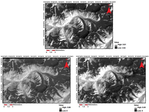
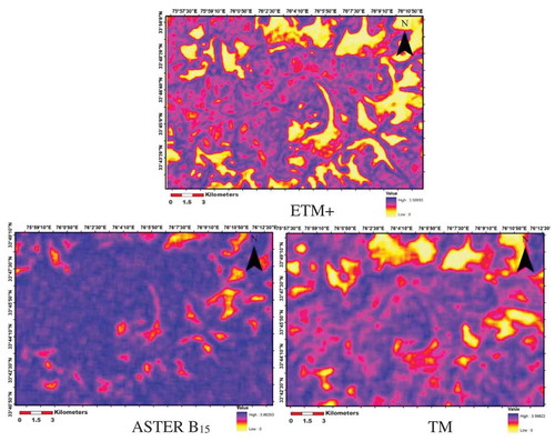
Figure 3. Top of Atmospheric Radiance Images: (A) ETM+ (B) ASTER B₁₅ (C) TM.

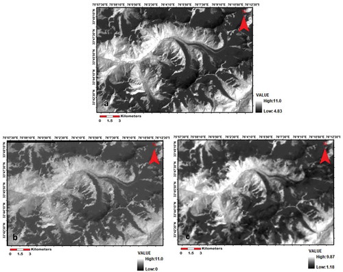
Figure 4. Surface Radiance Images: (A) ETM+ (B) ASTER B₁₅ (C) TM.

Remote sensing data have been used to help model surface temperatures specifically, validating LST data with actual on-the-ground temperature measurements. Thermal infrared (TIR) sensors are capable to acquire quantitative, quality information of surface temperature data about the evapotranspiration, climate change, hydrological cycle, vegetation monitoring, urban climate and environmental studies using single-infrared channel method or the split window method, depending on the number of bands used (Pu et al. 2006). With the use of high-resolution satellite data, it has become possible to monitor the global climate change and its impact on cryosphere both on continental or global scales, which is difficult with in situ measurements. Numerous studies have been carried out, and different approaches have been proposed to derive LSTs from satellite TIR data (Tang et al. 2008; Benali et al., 2012; Li et al. 2013; Williamson et al. 2014; Tang et al. 2015; Shen et al. 2016). Satellite measurements provide better results as compared to results obtained from interpolation of temperature data from sparsely located meteorological observatories. The primary objective of the present study is to (i) determine the land surface temperature using different techniques. (ii) Inter-comparison of the results. (iii) Analyse the influence of varying sensor characteristics on derived LST.

Study area

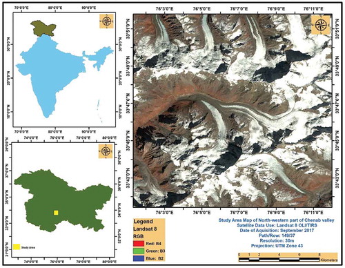
The study area is located in the north-western part of Chenab valley and extends from latitude 33°49ʹ39” N to 33°40ʹ23” N and 75°57ʹ11” E to 75°57ʹ09” E longitude (Figure 1). It lies along the north-eastern foothills of the Great Himalayan Wall, extending from Kargil town, and stretches southwards for a length of about 75 km to Panikhar, then eastward for another stretch of nearly 65 km to the foot of the Pensila watershed where the Suru River rises. The area has the Suru valley in its east, Nun and Kun peaks towards the north, Sarbal in its south and Marwah in its west. The area is located near the Suru valley, about 250 km (160 mi) east of Srinagar, the state summer capital.

Figure 1. Location Map of the Study Area (North-western part of Chenab valley J&K, India).

Data sets

For computations of Land surface temperature (LST) of the study area the thermal infrared (TIR) remote sensing data from Landsat 5 TM (acquired on August 27 2000), Landsat 7 ETM+ (acquired on 4 September 2000) and Terra ASTER (acquired on 4 September 2000) sensors were used. While selecting the remote sensing data for the study, importance was given that there should be minimal time-lag between the images acquired by different sensors otherwise the temperature data derived would not be comparable. The spectral bandwidth of the thermal bands for both TM and ETM is 10.4–12.5 µm and ASTER sensor has five thermal bands within a wavelength range from 8 to 12 µm (Table 1). A standard kinetic temperature in case of ASTER LST product (AST08) for 4 September 2000, was used as reference data for the present study.

Table 1. Detailed information of the Data sets used.

Type of data	Date of Acquisition	Spatial resolution Band wise	Band width (µm)	Quantization levels (bits)
Landsat-TM	27 August 2000	120	10.45–12.42	8
Landsat-ETM+	4 September 2000	60	10.31–12.36	8
ASTER B11	4 September 2000	90	8.12–8.47	12
ASTER B12	4 September 2000	90	8.4–8.8	12
ASTER B13	4 September 2000	90	8.9–9.7	12
ASTER B14	4 September 2000	90	10.2–10.9	12
ASTER B15	4 September 2000	90	10.9–11.6	12

Methodology

Most of the pre-processing work was done using ERDAS Imagine 14, which includes the execution of atmospheric, temperature estimation models, while the temperature emissivity separation and entropy estimation were done by using ENVI 4.1 and Arc GIS 10.1 was mainly used to prepare layouts of the results obtained as well as for the derivation of pixel values for temperature images. Before satellite imagery can be used as a data source the raw sensor data were processed to derive useful information from the digital numbers produced by using most basic and important processing techniques of geometric and radiometric correction. An image-to-image registration was conducted between the ASTER, TM and the ETM+ datasets while taking ETM+ as a reference image. Then using the classification-based emissivity approach these were converted to the surface temperature. Thereafter, several approaches, namely, entropy estimation, analysis of the spatial profiles, statistical analysis (standard deviation, correlation coefficient, RMSE, NRMSE) and resampling techniques had been employed to determine the influence of different spatial and radiometric resolutions of the sensors on the estimated temperatures. The schematic methodology for LST estimated flowchart is shown in (Figure2).

Figure 2. Schematic flowchart methodology used for LST estimation.

Radiometric corrections

For a scene to scene radiometric correction radiometric balancing need to be carried out if the data falls in two or more paths or belong to the different dates of acquisition. The first step of the radiometric correction of Landsat and ASTER images was to convert the digital numbers (DNs) of their bands into calibrated radiance values and atmospheric correction of the top of atmospheric radiance images (Figure 3).

Digital number (DN) to top of atmospheric radiance (TOA)

The Landsat Thematic Mapper (TM) and Enhanced Thematic Mapper Plus (ETM+) sensors acquire temperature data and store this information as a digital number (DN) with a range between 0 and 255 (D. Jovanović et al. 2015). This range is converted to radiance value before further processing (Chander and Markham 2003). The method of radiance evaluation is given below:

The formula to convert DN to radiance using gain and bias values (Table 2) for Landsat images is:

(1) $C{V}_{R1}=GAIN\ast DN+BIAS$(1)

Where:

CV_R1 is the cell value as radiance

DN is the cell value digital number

Gain is the gain value for a specific band

Bias is the bias value for a specific band

For aster radiance (Table 3) can be obtained from DN values as

(2) $C{V}_{R1}=\left(DN-1\right)\ast UCC$(2)

Where:

CV_R1 is the cell value as radiance

DN is the cell value digital number

UCC is the unit conversion coefficient

Atmospheric correction

Many factors affect the retrieval of LST from satellite thermal infrared data but some of them, such as transmittance, air moisture, downwelling and upwelling radiance, are usually difficult to obtain, especially from satellite observations (Figure 4 and Table 4). An atmospheric correction tool has been developed on a public access website for the thermal band sensors. The Atmospheric Correction Parameter Calculator uses the National Centres for Environmental Prediction (NCEP) modelled atmospheric global profiles interpolated to a particular date, time and location as input. With the help of MODTRAN radiative transfer code and a suite of integration algorithms, the site-specific atmospheric transmission, and upwelling and downwelling radiances are derived (Barsi, et al 2005).

From Coll, Caselles, and Galve (2005), the formula to apply scene-specific atmospheric correction is:

(3) $CV{R}_2=\frac{CV{R}_1}{\epsilon \tau }L\uparrow -\frac{1-\epsilon L\downarrow }{\epsilon }$(3)

Where:

CVR₂ is the atmospherically corrected radiance/surface radiance

CVR₂ is the (TOA);

L↑ is upwelling Radiance

L↓ is downwelling Radiance

τ is transmittance

ε is emissivity (typically 0.97)

Image processing

Image processing deals with the various procedures applied to an image after pre-processing in order to extract the required information from the image. Various image processing techniques applied in the present study are described in the following sections. Here the image processing techniques mainly comprise of land surface temperature retrieval techniques. These techniques basically include the temperature emissivity separation (TES) algorithms and other techniques of temperature estimation.

Temperature emissivity separation (TES) algorithms

The main approaches to estimate (LST) are to first separate the effect of the intervening atmosphere and then decouple (LST) and (LSE). The radiance emitted from a surface in the thermal infrared wavelength is a function of both the surface temperature and emissivity. TES accuracy, extensively assessed by simulations, remains for multiband simulations (within about 0.03 for emissivity and within about 1.2k (0.3k) for temperature. TES algorithm hybridizes three established algorithms, first estimating the emissivity’s and then calculating emissivity band ratios. An empirical relationship predicts the minimum emissivity from the spectral contrast of the rationed values, permitting recovery of the emissivity spectrum.

Reference channel technique

This method was developed by Kahle, Madura, and Soha (1980). It assumes that emissivity in one channel has a constant value for the entire image. The surface temperature is obtained from the selected channel for each pixel, the temperature calculated serves for the remaining channels emissivity calculation (Hosseinjani Zadeh and Tangestani 2013). Although this is the simplest method for the emissivity retrieval it suffers from some limitations. First, it is difficult to find a unique emissivity value that is appropriate for all surface materials in one reference channel. Secondly, because the emissivity is assigned as a constant value for all pixels there is no emissivity spatial information in this channel.

Emissivity normalization technique

This technique was developed by Gillespie (Gillespie et al. 1999). This technique assumes a fixed emissivity value and produces emissivity and temperature outputs and the maximum temperature for each pixel is used to compute the emissivity values using the Planck function. This method is an improvement of (RCM) as the channel with the maximum emissivity can be different in it for different materials.

Other LST estimation approaches

These are those methods of LST retrieval techniques which do not assume single emissivity values for the image and require it as one of the inputs for estimating surface temperatures. Two such techniques which have been used in this work are discussed below:

Classification-based approach

Generally, the classification-based emissivity method is based on the use of conventional information. The key point of this method is to properly classify the land surface and then to assign the emissivity from classification-based lookup tables for the given classes (Figure 5). Maximum likelihood classification algorithm has been used for delineation of six different classes (water, ice, snow, vegetation, barren land and debris) on a glacier terrain. The pixels in the images resulting from the maximum likelihood classification that represented water were given emissivity values of 0.99, pixels that represented ice were assigned a value of 0.97, snow pixels were given a value of 0.99, pixels representing vegetation, barren land and debris were given emissivity values of 0.98, 0.90 and 0.94, respectively. Theoretically, the classification-based emissivity method can produce accurate land surface emissivity products over the areas in which land surfaces are accurately classified and where each class has the well-known emissivity (Figure 6). In other words, the classifier-based emissivity prediction is thought to be accurate for most classes, especially for high resolution remotely sensed data (pure pixels). The emissivity values used in this case for each class are given below (Table 5).

Table 2. Gain and Bias values used (Source: https://landsat.usgs.gov/calibration).

USGS Landsat Calibration Values
Sensor Type	Gain Value	Bias Value
Landsat TM	0.055376	1.18
Landsat ETM+	0.067087	0.07

Table 3. UCC values used (Source: Abrams and Hook 2001).

UCC Values for ASTER Image
Band11	0.006822
Band12	0.00678
Band13	0.00659
Band14	0.00569
Band15	0.00522

Table 4. Atmospheric profile values acquired from web-based atmospheric correction parameter calculator (Source: http://www.ncep.noaa.gov/).

Sensor Type	Upwelling Radiance	Downwelling Radiance	Atmospheric Transmittance	Emissivity
Landsat TM	1.31	2.14	0.81	0.97
Landsat ETM+	1.15	1.89	0.82	0.97
ASTER	1.15	1.89	0.82	0.97

Table 5. Emissivity values of different land cover features used.

In-situ emissivity values for 10–12 µm wavelength
Water	0.99
Ice	0.97
Snow	0.99
Vegetation	0.98
Barren land	0.90
Debris	0.94

Figure 5. Classified image.

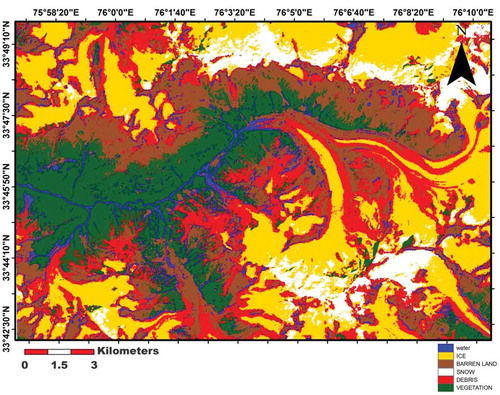
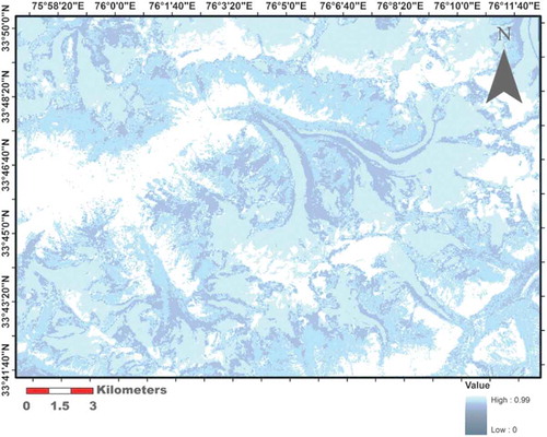
Figure 6. Emissivity Map.

Once the emissivity map of the area is derived then the equation used for land surface derivation is as under:

(4) $LST=\frac{K2}{ln\left(\frac{K1}{CV{R}_2}+1\right)\ast \epsilon }$(4)

Where:

LST is the land surface temperature

CVR₂ is the atmospherically corrected radiance/surface radiance

ε is the emissivity map of the area

K₁ and K₂ are the pre-calibrated constants

The tabulated pre-calibrated constant values have been taken from handbook data pertaining to each sensor (Table 6).

Table 6. Pre-calibrated constant values (Abrams and Hook 2001).

Sensor type	K1	K2
Landsat TM	607.76	1260.56
Landsat ETM+	666.09	1282.71
ASTER B11	3040.13	1735.33
ASTER B12	2482.37	1666.39
ASTER B13	1935.06	1585.42
ASTER B14	866.46	1350.06
ASTER B15	641.32	1271.22

Technique based on Stefan-Boltzmann law

Satellite thermal infrared sensors measure radiances at the top of the atmosphere, from which brightness temperatures TB (also known as blackbody temperatures) can be derived by using Plank’s law (Markham et al., 1986). With the known LSE, the emissivity-corrected LST (TS) can be calculated by the Stefan Boltzmann law (Gupta 1991) (Figure 7).

(5) $T_B=\epsilon \sigma LS{T}^4$(5)

Figure 7. Brightness temperature images: (a) ETM+ (b) ASTER B15 (c) TM.

Therefore

(6) $LST=\frac{1}{\in 1/4}TB$(6)

Where:

TB is the brightness temperature

LST is the land surface temperature

ε is the emissivity map of the area

σ is the Stefan Boltzmann constant (5.67 x 10⁻⁸ Wm⁻² K⁻⁴)

Results & discussions

Intercomparing & accuracy assessment of LST estimation techniques

For the purpose of selecting the most appropriate LST derivation technique, an accuracy assessment was carried between the derived land surface temperature images and (ASTER08) temperature image used as a reference image (Figure 8). Following statistical accuracy, measures were used for this purpose correlation accuracy assessment root-mean-square error and normalized root-mean-square (NRMNS) accuracy assessment.

Figure 8. ASTER 08 Image.

Accuracy assessment for ASTER (LST) images

This accuracy assessment has been carried out between the derived land surface temperature images of ASTER B₁₅ and the reference image. The four ASTER LST images estimated through different techniques are shown in (Figure 9).

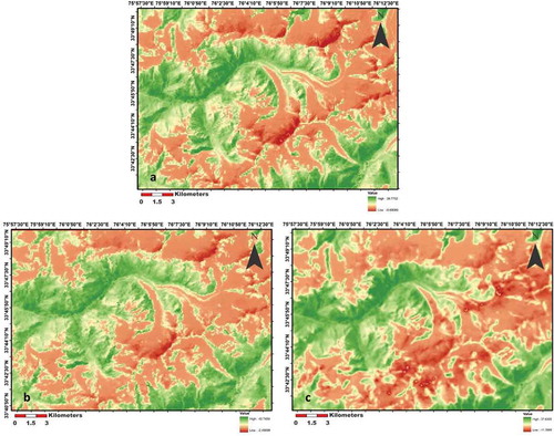
Figure 9. Derived LST images for ASTER B₁₅ (Keywords: (CBA) Classification-based Approach, (SBL) Stefan Boltzmann’s Law, (NEM) Normalization Emissivity Method, (RCM) Reference Channel Method.

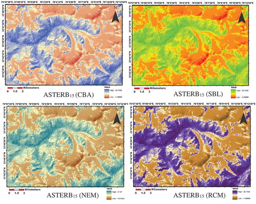
Histogram statistical analysis for ASTER B₁₅ LST images

This accuracy assessment is simply the comparison of the histogram statistics pertaining to each senor-based land surface temperature with the reference data. The histogram statistical data of ASTER B₁₅ for each LST derived technique and the reference image are shown below (Table 7). From these data, it is clear that the land surface temperature estimated through a classification-based approach shows more close proximity than the LST images estimated by other techniques.

Table 7. Histogram statistical data pertaining to derived ASTER images and the reference image.

Sensor Type	Minimum value	Maximum value	Mean value	Median	Mode value	Standard deviation
ASTERB15(CBA)	−4.4	38.7	15.3	13.9	6.1	9.6
ASTERB15 (SBL)	−4.4	38.7	15.4	14.08	6.1	9.5
ASTERB15 (NEM)	−16.5	31.07	6.02	4.1	−0.16	10.2
ASTERB15 (RCM)	−16.5	31.07	6.02	4.1	−0.1	10.2
ASTER08	−12.05	42.5	14.2	13.1	2.2	11.8

RMSE, NRMSE and correlation accuracy assessment for ASTER B₁₅ (LST) image and reference image

Normalized root Mean square error (NRMSE), Root mean square error (RMSE) and Correlation techniques are used for the accuracy assessment of the derived LST images of ASTER and reference image (Table 8). From its interpretation, it is observed that the correlation is highest between the classification-based approach derived LST image and the reference image which is followed by the Stefan Boltzmann’s law-based approach whereas there is no such deviation afterwards. The other parameters of the accuracy assessment show the similar trend. Thus, from this it is it again proves the supremacy of the classification-based approach for LST estimation.

Table 8. NRMSE, RMSE and correlation values for ASTER B₁₅ (LST) images. (Keywords: (CBA) Classification Based Approach, (SBL) Stefan Boltzmann’s Law, (NEM) Normalization Emissivity Method, (RCM) Reference Channel Method.

Sensor Type	Correlation	RMNS	NRMNS	Percentage NRMNS
ASTER B15(CBA)	0.94	5.6	0.11	11.9
ASTER B15(SBL)	0.93	5.7	0.12	12
ASTER B15(NEM)	0.88	6.6	0.15	15
ASTER B15(RCM)	0.88	6.6	0.15	15

Accuracy assessment for ETM+ (LST) images

This accuracy assessment has been carried out between the derived land surface temperature images of ETM+ and the reference image. The four ETM+ LST images estimated through different techniques are shown in (Figure 10).

Figure 10. Derived ETM+ images for ASTER B₁₅ (Keywords: (CBA) Classification-based Approach, (SBL) Stefan Boltzmann’s Law, (NEM) Normalization Emissivity Method, (RCM) Reference Channel Method.

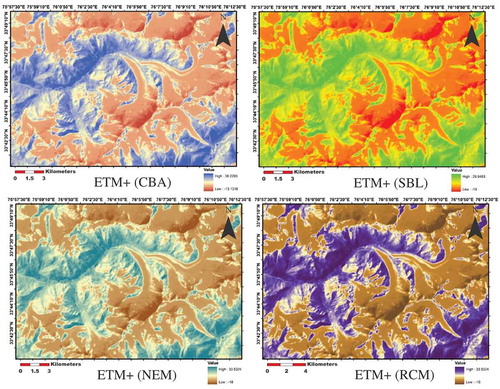
Histogram statistical analysis for ETM+ LST images

This accuracy assessment has been carried out between the histogram statistical data of derived land surface temperature images of ETM+ and the reference image (ASTER08). The histogram statistical data of ETM+ for each (LST) derived technique and the reference image are given below (Table 9). From these data, it is again clear that the land surface temperature estimated through a classification-based approach shows more close proximity than the LST images estimated by other techniques.

Table 9. Histogram statistical data pertaining to derived ETM+ images and reference image.

Sensor Type	Minimum value	Maximum value	Mean value	Median	Mode value	Standard deviation
ETM+ (CBA)	−13.1	38	11.5	10.3	1.5	10.4
ETM+ (SBL)	−19	29.9	0.8	−0.14	−10.1	11.19
ETM+ (NEM)	−18	33.5	3.3	2.07	−8	11.9
ETM+ (RCM)	−19	31.2	1.5	0.23	−9.8	11.8
ASTER08	−12.05	42.5	14.2	13.1	2.2	11.8

RMSE, NRMSE and correlation accuracy assessment for ETM+ (LST) image and reference image

Normalized root Mean square error (NRMSE), Root mean square error (RMSE) and Correlation techniques used for the accuracy assessment of the derived LST images of ETM+ and reference image (Table 10). From its interpretation, it is again observed that the correlation is highest between the classification-based approach derived LST image and the reference image which is followed by the normalization emissivity method and reference channel method both shows equal values and the correlation is least for the Stefan Boltzmann’s law-based approach. However, there is the variation in the values obtained when compared to the values obtained for ASTER LST images which could be attributed due to the variation in the sensor characteristics.

Table 10. NRMSE, RMSE and correlation values for ASTER B₁₅ (ETM+) images. (Keywords: (CBA) Classification Based Approach, (SBL) Stefan Boltzmann’s Law, (NEM) Normalization Emissivity Method, (RCM) Reference Channel Method.

Sensor Type	Correlation	RMNS	NRMNS	Percentage NRMNS
ETM+ (CBA)	0.91	6.3	0.16	16.8
ETM+ (SBL)	0.75	13.2	0.36	36
ETM+ (NEM)	0.82	10.2	0.27	27.3
ETM+ (RCM)	0.82	10.2	0.27	27.3

Accuracy assessment for TM (LST) images

This accuracy assessment has been carried out between the derived land surface temperature images of TM and the reference image. The four TM LST images estimated through different techniques are shown in (Figure 11).

Figure 11. Derived TM images for ASTER B₁₅ (Keywords: (CBA) Classification Based Approach, (SBL) Stefan Boltzmann’s Law, (NEM) Normalization Emissivity Method, (RCM) Reference Channel Method.

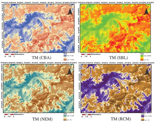
Histogram statistical analysis for TM LST images

This accuracy assessment has been carried out between the histogram statistical data of derived land surface temperature images of TM and the reference image (ASTER 08). The histogram statistical data of TM for each (LST) derived technique and the reference image (Table 11). From its interpretation, it has been found that except the standard deviation value for the classification-based approach the other statistical parameters of the histogram statistics are highly related when compared to the relative histogram parameters obtained from other techniques. The sharp decrease in the minimum and maximum values compared to the reference image could be attributed to its low resolution and variation in the date of acquisition of an image. The trend followed for close proximity of histogram statistical data is a classification-based approach followed by temperature emissivity method (NEM, RCM) and least by Stefan Boltzmann law-based approach.

Table 11. Histogram statistical data pertaining to derived ETM+ images and reference image.

Sensor Type	Minimum value	Maximum value	Mean value	Median	Mode value	Standard deviation
TM (CBA)	−15.1	31.4	6.5	4.2	−1.3	10
TM (SBL)	−26	20	−7.1	−9.5	−16.1	10.9
TM (NEM)	−25	21.07	−6.7	−9.3	−16.8	11.17
TM (RCM)	−26	21.07	−6.7	−9.3	−16.8	11.17
ASTER08	−12.05	42.5	14.2	13.1	2.2	11.8

RMSE, NRMSE and correlation accuracy assessment for TM (LST) image and reference image

Normalized root Mean square error (NRMSE), Root mean square error (RMSE) and Correlation techniques used for the accuracy assessment of the derived LST images of TM and reference image (Table 12). By interpreting the figures, the trend observed for the given techniques is as classification-based approach shows high close proximity with the reference image data followed by the normalization-based approach and reference channel method and least by Stefan Boltzmann law-based approach. The sharp dip in the values compared to other sensor type images is again due to its low spatial resolution and variation in the date of acquisition of an image.

It is evident the classification-based approach has shown high correlation with the reference image in order of ASTER B₁₅ > ETM+> TM. Although it was expected that the correlation between the derived ASTER image and reference ASTER image should have one correlation which has not been the case and it has been attributed due to the variation in temperature estimation approach and partly due to the band used in reference image, whereas in the other two sensor types the variation has been attributed due to the sensor characteristics.

Table 12. NRMSE, RMSE and correlation values for ASTER B₁₅ TM images. (Keywords: (CBA) Classification Based Approach, (SBL) Stefan Boltzmann’s Law, (NEM) Normalization Emissivity Method, (RCM) Reference Channel Method.

Sensor Type	Correlation	RMNS	NRMNS	Percentage NRMNS
TM (CBA)	0.83	11.7	0.31	31.1
TM (SBL)	0.60	14.8	0.40	40
TM (NEM)	0.75	12.3	0.35	35.6
TM (RCM)	0.75	12.3	0.35	35.6

Impact of the sensor characteristics on the land surface temperature

At this stage, the generated LST maps selected after intercorrelation and normalized root mean square error analysis between different approaches used and the reference data are analysed for the radiometric as well as spatial analysis based on certain approaches to evaluate the results.

Re-scaled (LST) image derivation and its inference on sensor characteristics

Both ETM+ and TM data were re-scaled to the scale of 90 meters. The aim of this process was to bring the spatial extent of the pixels of all the three data sets to a common scale (ASTER spatial resolution). After this processing land surface temperature was estimated for ETM+ and TM by using the classification-based approach. The temperature images generated after are given below (Figure 12).

Figure 12. Re-scaled ETM+ & TM.

The histogram statistical data pertaining to the rescaled ETM+, TM and ASTER08 image which have been assessed for their inference on the sensors varying characteristics (Table 13). From this data, it is clear that after changing the spatial resolution of the ETM+ and TM image their temperature value is approaching closer to the ASTER LST image although there is a little deviation in case of the ETM+ and more deviation in TM LST image. In this approach of assessment, the estimated LST image was correlated with the earlier LST derived images for each sensor, in the idle condition it was indented that correlation will be equal to one which means that by changing the spatial extent of the cell or in other words spatial resolution has no effect on the LST values of the pixel. The other results possible are that correlation will not be equal to one thus proving the effects of spatial resolution on the derived LST values. In this case, the ETM+ and TM LST image derived after re-scaling the image to a common spatial resolution of 90 m was correlated with the LST derived image of the ASTER. For no effect of radiometric resolution on the LST images, it was expected that the re-scaled LST images of the ETM+ and TM will have a correlation of one with the ASTER-derived LST image or vice versa in case the radiometric resolution does the effect. To quantify the effect pixel-based assessment was carried out and the results derived for correlation, (NRMSE) and (RMSE) techniques. The correlation and average deviation between the pixel values of rescaled ETM+ and original ETM+ LST image, similarly with ASTER LST image are shown in the below (Table 14).

Table 13. Statistical data for Re-scaled ETM+, TM and ASTER08.

Sensor Type	Minimum value	Maximum value	Mean value	Median	Mode value	Standard deviation	Range
ETM+	−11.93	41.4	13.3	12.2	2.2	11.6	53.3
TM	−14.8	35.6	7.8	4.8	−1.2	10	50.4
ASTER08	−12.05	42.5	14.2	13.1	2.2	11.8	54

Table 14. Estimated correlation and average deviation values for re-scaled image.

Class Type	Correlation with ETM+	Average deviation	Correlation with ASTER B15	Average deviation
Barren Land	0.85	2.4	0.61	1
Snow	0.84	0.48	0.71	4.5
Vegetation	0.97	3.7	0.96	2.6
Water	0.97	3	0.70	1.1
Debris	0.88	2	0.73	2.9
Ice	0.54	0.52	0.65	4.3

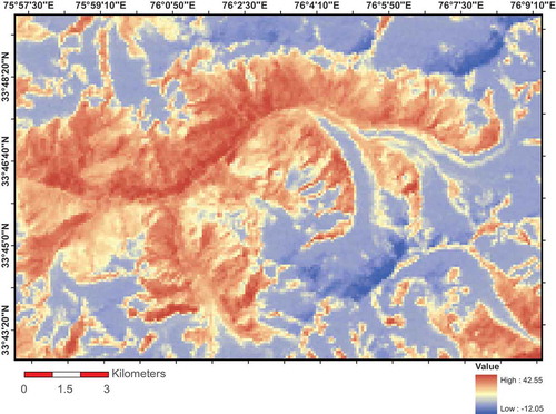
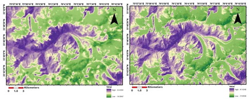
Entropy image estimation and its inference on sensor characteristics

To estimate the effect of radiometric resolution on the derived LST images entropy image for all the three data sets were derived. Statistical comparison was then carried out between the derived entropy images to ascertain the effect on each sensor type land surface temperature. Entropy image was derived for each LST images to know the effect of radiometric resolution on the derived LST images. Entropy which is defined as the degree of randomness should increase with an increase in the energy levels of the pixel. A general perception was carried for this assessment that is as the radiometric resolution of the data increases the entropy of the image should also increase. In this case, the entropy of the ETM+ and TM was expected to be the same due to the same radiometric resolution and that for the ASTER should increase due to high radiometric resolution. From the mode value of the entropy image shown below, it is been observed that the entropy of the ASTER is higher than the ETM+ and TM which has been attributed due to the high radiometric resolution of the ASTER (Table 15). The little increase in the mode value of TM could be attributed to the temporal effect. Thus, in conclusion, entropy of the image increases with the increase in the radiometric resolution (Figure 13).

Table 15. Statistical figures for Entropy images.

Entropy image	Maximum value	Mean value	Median	Mode value	Standard deviation
ETM	3.5	2.3	2.5	2.5	0.79
ASTER B15	3.8	3.2	3.6	3.6	0.82
TM	3.5	2.5	2.8	2.8	0.85

Figure 13. Entropy images.

Spatial profile assessment

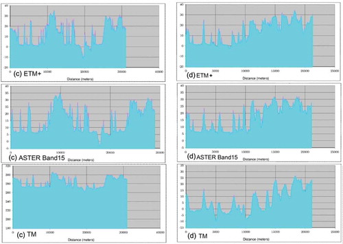
Spatial profile of LST images for a fixed area was drawn for each sensor data representing the effect of almost all the classes from the study area. Then, each spatial profile was assessed to quantify the differences among them thus showing the effects of spatial resolution. To start with four different-sized line segments were drawn on the LST images procured from each sensor. These segments were named as A, B, C and D (Figure 14). While drawing these line segments it was taken into consideration that all these line segments will represent the effect of different features in the study area. Spatial profiles of these line segments were then assessed for the effect of variation in the LST image for spatial resolution. From the profiles given below it is found that the ETM+ LST image shows more peaks followed by ASTER and finally to TM and from this observation it is referenced that the high-resolution ETM+ images capture the heterogeneous effect of the feature very well contrary to the other two sensors which assume the area as homogeneous thus averaging the temperature value of the area which in turn does affect the accuracy of the LST value observed at micro level. This assessment was done by observing the number of peaks of each line segment overlaid over the derived land surface temperature image for each sensor type. The different line segments have taken for the task followed by the spatial profiles of these line segments for each sensor data I shown in (Figure 15 (a–d)).

Figure 14. Location of line segments used for spatial profile.

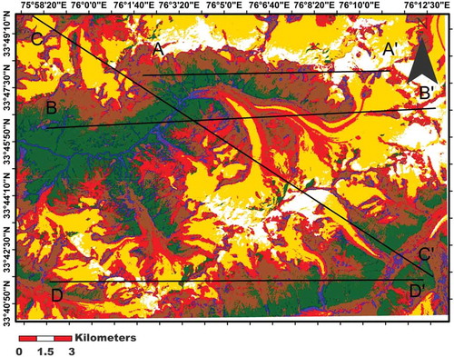
Figure 15. (a): Spatial profile for line segment A for Landsat ETM+, ASTER B₁₅, Landsat TM sensor typed LST image. (b): Spatial profile for line segment B for Landsat ETM+, ASTER B₁₅, Landsat TM sensor typed LST image. (c): Spatial profile for line segment C for Landsat ETM+, ASTER B₁₅, Landsat TM sensor typed LST image. (d): Spatial profile for line segment D for Landsat ETM+, ASTER B₁₅, Landsat TM sensor typed LST image.

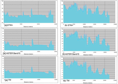
Figure 15. (Continued).

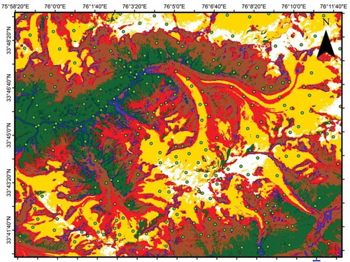
Pixel-based assessment

The pixel-wise assessment was carried out between the estimated temperature data of each sensor. About three hundred points were used for this observation distributed all over the image thus taking into consideration the various classes in the study area (Figure 16). The pixel value of all these points were recorded for each sensor data. The deviation between the pixel values of ETM+ and TM has directly attributed due to the effect of the spatial resolution were as the deviation between the ETM+ and ASTER was attributed due to the effect of both low spatial resolution as well as due to high radiometric resolution. Average deviation value for each class between the ETM+ and TM and similarly between the ETM+ and ASTER was then calculated. The average deviation obtained for each class type due to the spatial resolution effect between the ETM+ and TM LST image is shown in the (Table 16).

Table 16. Average deviation values between ETM+ and TM.

Sensor Type	Class type	Average deviation
ETM+	Barren land	3.27
	Snow	4
	Ice	3.06
TM	Debris	3.32
	Vegetation	4.33
	Water	3.2

Figure 16. Observed Points.

The variation in the average value of different classes could be attributed due to the homogeneity and heterogeneity of the class and the emissivity value is taken for the same. The average deviation obtained for each class type due to the spatial and radiometric resolution effect between the ETM+ and ASTER B₁₅ LST image (Table 17).

Table 17. Average deviation between ASTER B₁₅ and ETM+.

Sensor Type	Class type	Average deviation
ETM+	Barren land	4.7
	Snow	4.3
	Ice	5
ASTER B15	Debris	3.4
	Vegetation	2.7
	Water	3.5

Normalized root-mean-square error (NRMS) assessment

The deviation values obtained in pixel-based assessment for each sensor temperature data to quantify the values in terms of the RMSE, NRMSE and percentage NRMSE .in this case of assessment the reference image used is ETM+ and coefficient values obtained were between ETM+ and TM which is due to spatial resolution effect and the coefficient values obtained for ETM+ and ASTER B₁₅ were attributed due to both spatial as well as radiometric effect. The results obtained are tabulated are given below (Table 18). By observing the values for (RMSE) and NRMSE it is clear that efficiency is low for spatial resolution (between ETM+ and TM) and higher for both spatial as well as the radiometric resolution between ETM+ and ASTER LST image. Now if we here intend to exactly estimate the effect of radiometric resolution for that purpose we need to estimate the effect of spatial resolution for the results estimated for ETM+ and ASTER temperature image which needs some mathematical simplifications like subtraction and division to exactly estimate the (RMSE) and (NRMSE) values for radiometric resolution.

Table 18. RMSE, NRMSE values of ETM+ with TM and ASTER image.

Values with	RMSE	RMSE	Percentage Error
TM	4.25	0.12	12
ASTER B15	4.47	0.13	13

Conclusion

• This study has used TIR band of all the three mentioned sensor data for land surface temperature estimation. Besides the advantage of their high spatial resolution, the varying sensor characteristic features gave us insight into the variation in their accuracy for land surface temperature determination. Different Techniques were used for the estimation of Land surface temperature from satellite data and it was found that classification-based temperature estimation is more accurate technique in terms of its accuracy level as depicted by statistical figures estimated through correlation, NRMSC and RMSE techniques used for multi-sensors the classification-based approach has shown high correlation with the reference image in order of ASTER B₁₅ > ETM+> TM.

• The statistics derived from the entropy images of the three TIR sensors, especially the mean value, clearly indicate that the information content of ASTER-derived LST image were highest as compared to the other two. Moreover, the spatial distribution of entropy values suggests that ASTER-derived LST images depict higher entropy values even on the glaciered portion i.e. snow-ice part, where the ETM+ and TM images show distinctively lower entropies. This means that ASTER TIR data owing to its higher radiometric resolution (12 bit) is able to better characterize even small variations in homogeneous land covers such as snow-ice.

• Spatial profiles drawn on the LST images derived from the three sensors revealed that ETM+ data was able to capture the temperature variations in the heterogeneous classes like vegetation and rock exposures which characterize the non-glaciated areas and cover broad temperature ranges. This is possibly due to the high spatial resolution of the ETM+ data. However, the ASTER B₁₅ data, owing to its high radiometric resolution, is able to highlight even the subtle temperature changes in the homogeneous classes like snow and ice (i.e. the glaciated terrain). Comparison of statistics derived from the LST images of the three sensors with the AST08 (T_mean = 14.2°C) reference image shows that ASTER B₁₅ data (T_mean = 15.3°C) matches closely, while ETM+ (T_mean = 11.5°C) and TM (T_mean = 6.5°C) show large deviations. Correlation, root mean squared error (RMSE) and normalized RMSE (NRMSE) between the LST images with the reference image also corroborate the above observations.

• Both ETM+ and TM data were re-scaled to the scale of 90 m. The aim of this process was to bring the spatial extent of the pixels of all the three data sets to a common scale (ASTER spatial resolution). From this data it is clear that after changing the spatial resolution of the ETM+ and TM image their temperature value is approaching closer to the reference image. Also, the correlation of resampled ETM+ LST image with ASTER B₁₅ still comes to only 0.73, which ideally (if there is no effect of radiometric resolution) should have been 1 after resampling.

• Variation in average deviation value for different class types could be attributed due to the mixing of spectral radiance with other classes present near measurement site on the spatial scales of the class and subsequently the closeness of the emissivity value used. Moreover, the variation due to spatial resolution effect for the classes has a direct link with the topography of the area if the area representing a feature class is present in a more rugged terrain more the variation it would show due to spatial resolution effect. Quantifying the exact deviation due to the radiometric resolution effect is not possible unless other characteristic features of the sensor are not estimated.

Compliance with ethical standards

Compliance with Ethical Standards This study is in full compliance with all applicable ethical standards.

Ethical Approval This research paper does not contain any studies with human participants or animals performed by any of the authors.

Informed Consent Each author contributed to the research in terms of conception, research design, cross-checking data analysis and co-writing the paper.

Acknowledgments

Authors would like to thank LP DAAC, US Geological Survey (USGS), National Aeronautics and Space Administration (NASA) and NASA’s Earth Observing System Data and Information System (EOSDIS) for assessing high-resolution satellite data. Special thanks to the editor in chief (Dr A-Xing Zhu) and anonymous reviewers for their constructive comments to improve this article.

Disclosure statement

No potential conflict of interest was reported by the authors.

References

- Abrams, H., and S. Hook. 2001. ASTER User Handbook. CA, USA: Jet Propulsion Laboratory Pasadena.
- Barsi, J. A., J. R. Schott, J. R. Schott, F. D. Palluconi, F. D. Palluconi, S. J. Hook, and S. J. Hook. 2005. “Validation of a Web-Based Atmospheric Correction Tool for Single Thermal Band Instruments.” Proc. SPIE 5882, Earth Observing Systems X, 58820E, August 22. doi: 10.1117/12.619990
- Benali, A. C., J. P. Carvalho, N. N. Carvalhais, and A. Santos. 2012. “Estimating Air Surface Temperature in Portugal Using MODIS LST Data.” Remote Sensing of Environment 124 (12): 108–121. doi:10.1016/j.rse.2012.04.024.
- Chander, G., and B. Markham. 2003. “Revised Landsat-5 Tm Radiometric Calibration Procedures and Post Calibration Dynamic Ranges.” IEEE Transactions on Geoscience and Remote Sensing 41: 2674–2677. doi:10.1109/TGRS.2003.818464.
- Coll, C., V. Caselles, and J. M. Galve. 2005. “Ground Measurements for the Validation of Land Surface Temperatures Derived from AATSR and MODIS Data.” Remote Sensing of Environment 97: 288–300. doi:10.1016/j.rse.2005.05.007.
- Feizizadeh, B., T. Blaschke, H. Nazmfar, E. Akbari, and H. Kohbanani. 2013. “Monitoring Land Surface Temperature Relationship to Land Use/Land Cover from Satellite Imagery in Maraqeh County, Iran.” Journal of Environmental Planning and Management 56: 1290–1315. doi:10.1080/09640568.2012.717888.
- Gillespie, A. R., S. Rokugawa, S. J. Hook, T. Matsunaga, and A. Kahle 1999. Temperature/Emissivity separation algorithm theoretical basis document, version 2.4, ATBD-AST-05-08, Prepared under NASA contract NAS5-31372.
- Gupta, R. P. 1991. Remote Sensing Geology. Germany: Springer-Verlag Berlin Heidelberg.
- Hansen, J., R. Ruedy, M. Sato, and K. Lo. 2010. “Global Surface Temperature Change.” Reviews of Geophysics 48 (RG): 4004. doi:10.1029/2010RG000345.
- Hosseinjani Zadeh, M., and M. H. Tangestani. 2013. “Comparison of ASTER Thermal Data Sets in Lithological Mapping at A Volcano-Sedimentary Basin: A Case Study from South Eastern Iran.” International Journal of Remote Sensing 34 (23): 8393–8407. doi:10.1080/01431161.2013.838709.
- Jovanović, D., M. Govedarica, F. Sabo, D. Sladić, and A. Ristić. 2015. “Spatial Analysis of High-Resolution Urban Thermal Patterns in Vojvodina, Serbia, Geocarto International.” 30 (5): 483–505. doi:10.1080/10106049.2014.985747.
- Kahle, A. B., D. P. Madura, and J. M. Soha. 1980. “Middle Infrared Multispectral Aircraft Scanner Data: Analysis for Geological Applications.” Applied Optics 19 (14): 2279–2290. doi:10.1364/AO.19.002279.
- Kalma, J. D., T. R. McVicar, and M. F. McCabe. 2008. “Estimating Land Surface Evaporation: A Review of Methods Using Remotely Sensed Surface Temperature Data.” Surveys in Geophysics 29: 421–469. doi:10.1007/s10712-008-9037-z.
- Karnieli, A., N. Agam, R. T. Pinker, M. Anderson, M. L. Imhoff, and G. G. Gutman. 2010. “Use of NDVI and Land Surface Temperature for Drought Assessment: Merits and Limitations.” Journal of Climate 23: 618–633. doi:10.1175/2009JCLI2900.1.
- Li, Z., B. Tang, H. Wu, H. Ren, G. Yan, Z. Wan, I. F. Trigo, and J. A. Sobrino. 2013. “Satellite-Derived Land Surface Temperature: Current Status and Perspectives.” Remote Sensing Environment 131,: 14–37. doi:10.1016/j.rse.2012.12.008.
- Markham, B. L., and J. L. Barkewr. 1986. “Landsat MSS and TM Post Calibration Dynamic Ranges, Exoatmospheric Reflectance and At-Satellite Temperatures.” EOSAT Landsat Technical Notes 1,: 3–8.
- Orth, R., E. Dutra, I. F. Trigo, and G. Balsamo. 2017. “Advancing Land Surface Model Development with Satellite-Based Earth Observations.” Hydrology and Earth System Sciences 21: 2483–2495. doi:10.5194/hess-21-2483-2017.
- Penghai, W., H. Shen, L. Zhang, and F.-M. Göttsche. 2015. “Integrated Fusion of Multi-Scale Polar-Orbiting and Geostationary Satellite Observations for the Mapping of High Spatial and Temporal Resolution Land Surface Temperature.” Remote Sensing of Environment 156: 169–181. doi:10.1016/j.rse.2014.09.013. January.
- Pu, R., P. Gong, R. Michishita, and T. Sasagawa. 2006. “Assessment of Multi-Resolution and Multi-Sensor Data for Urban Surface Temperature Retrieval.” Remote Sensing of Environment 104: 211–225. doi:10.1016/j.rse.2005.09.022.
- Shen, H., L. Huang, L. Zhang, P. Wu, and C. Zeng. 2016. “Long-Term and Fine-Scale Satellite Monitoring of the Urban Heat Island Effect by the Fusion of Multi-Temporal and Multi-Sensor Remote Sensed Data: A 26-Year Case Study of the City of Wuhan in China.” Remote Sensing of Environment 172: 109–125. doi:10.1016/j.rse.2015.11.005.
- Tang, B., K. Shao, Z. Li, H. Wu, F. Nerry, and G. Zhou. 2015. “Estimation and Validation of Land Surface Temperature from Chinese Second Generation Polar-Orbiting FY-3A VIRR Data.” Remote Sensing 7: 3250–3273. doi:10.3390/rs70303250.
- Tang, B.-H., Y. Bi, Z.-L. Li, and J. Xia. 2008. “Generalized Split-Window Algorithm for Estimate of Land Surface Temperature from Chinese Geostationary Feng Yun Meteorological Satellite (FY-2C) Data.” Sensors 8: 933–951. doi:10.3390/s8010464.
- Trigo, I. F., S. Boussetta, P. Viterbo, G. Balsamo, A. Beljaars, and I. Sandu. 2015. “Comparison of Model Land Skin Temperature with Remotely Sensed Estimates and Assessment of Surface-Atmosphere Coupling.” Journal of Geophysical Research 120. doi:10.1002/2015JD023812.
- Weng, Q. 2009. “Thermal Infrared Remote Sensing for Urban Climate and Environmental Studies: Methods, Applications, and Trends (Review Article).” ISPRS Journal of Photogrammetry and Remote Sensing 64: 335–344. doi:10.1016/j.isprsjprs.2009.03.007.
- Williamson, S. N., D. S. Hik, J. A. Gamon, J. L. Kavanaugh, and G. E. Flowers. 2014. “Estimating Temperature Fields from MODIS Land Surface Temperature and Air Temperature Observations in a Sub-Arctic Alpine Environment.” Remote Sensing 6: 946–963. doi:10.3390/rs6020946.
- Wu, P., H. Shen, A. Tinghua, and Y. Liu. 2013. “Land-Surface Temperature Retrieval at High Spatial and Temporal Resolutions Based on Multi-Sensor Fusion.” International Journal of Digital Earth 6 (1): 113–133. doi:10.1080/17538947.2013.783131.